HAL Id: hal-03051699
https://hal.archives-ouvertes.fr/hal-03051699
Submitted on 10 Dec 2020
HAL is a multi-disciplinary open access
archive for the deposit and dissemination of
sci-entific research documents, whether they are
pub-lished or not. The documents may come from
teaching and research institutions in France or
abroad, or from public or private research centers.
L’archive ouverte pluridisciplinaire HAL, est
destinée au dépôt et à la diffusion de documents
scientifiques de niveau recherche, publiés ou non,
émanant des établissements d’enseignement et de
recherche français ou étrangers, des laboratoires
publics ou privés.
Robust Multiyear Climate Impacts of Volcanic
Eruptions in Decadal Prediction Systems
Leon Hermanson, Roberto Bilbao, Nick Dunstone, Martin Ménégoz, Pablo
Ortega, Holger Pohlmann, Jon Robson, Doug Smith, Gary Strand, Claudia
Timmreck, et al.
To cite this version:
Leon Hermanson, Roberto Bilbao, Nick Dunstone, Martin Ménégoz, Pablo Ortega, et al.. Robust
Mul-tiyear Climate Impacts of Volcanic Eruptions in Decadal Prediction Systems. Journal of Geophysical
Research: Atmospheres, American Geophysical Union, 2020, 125 (9), �10.1029/2019jd031739�.
�hal-03051699�
Leon Hermanson1 , Roberto Bilbao2 , Nick Dunstone1 , Martin Ménégoz3, Pablo Ortega2, Holger Pohlmann4,5 , Jon I. Robson6 , Doug M. Smith1 , Gary Strand7 ,
Claudia Timmreck5 , Steve Yeager7, and Gokhan Danabasoglu7
1Met Office, Exeter, UK,2Barcelona Supercomputing Center, Barcelona, Spain,3National Centre for Scientific
Research, Université Grenoble Alpes, Grenoble, France,4Deutscher Wetterdienst, Offenbach, Germany,5Max Planck Institute for Meteorology, Hamburg, Germany,6National Centre for Atmospheric Science, University of Reading,
Reading, UK,7National Center for Atmospheric Research, Boulder, CO, USA
Abstract
Major tropical volcanic eruptions have a large impact on climate, but there have only been three major eruptions during the recent relatively well-observed period. Models are therefore an important tool to understand and predict the impacts of an eruption. This study uses five state-of-the-art decadal prediction systems that have been initialized with the observed state before volcanic aerosols are introduced. The impact of the volcanic aerosols is found by subtracting the results of a reference experiment where the volcanic aerosols are omitted. We look for the robust impact across models and volcanoes by combining all the experiments, which helps reveal a signal even if it is weak in the models. The models used in this study simulate realistic levels of warming in the stratosphere, but zonal winds are weaker than the observations. As a consequence, models can produce a pattern similar to the North Atlantic Oscillation in the first winter following the eruption, but the response and impact on surface temperatures are weaker than in observations. Reproducing the pattern, but not the amplitude, may be related to a known model error. There are also impacts in the Pacific and Atlantic Oceans. This work contributes toward improving the interpretation of decadal predictions in the case of a future large tropical volcanic eruption.1. Introduction
Volcanoes have global impacts on climate from monthly to centennial timescales (Ding et al., 2014; Robock, 2000; Timmreck, 2012; Timmreck et al., 2016; Zhong et al., 2011). Volcanic impacts are needed to fully explain the climate variability of the twentieth century (Smith et al., 2016). Understanding these impacts can help with prediction and planning in the case of a volcanic eruption today. In the modern observational period, there have been three major tropical eruptions: Agung (1962), El Chichón (1982), and Pinatubo (1991).
When a volcanic eruption is powerful enough, such as the ones mentioned above, the volcanic plume reaches up into the stratosphere and aerosols formed there can remain for months to years. When the erup-tions are in the tropics, the aerosols are quickly spread across all longitudes by the strong winds in the stratosphere. Once in the stratosphere, the aerosols cause local warming. This is caused by shortwave absorp-tion and also by blocking of upward longwave radiaabsorp-tion (Hansen et al., 1997; Lacis et al., 1992; Swingedouw et al., 2017). In winter, the stratospheric warming modifies the midlatitude to polar temperature gradient, which strengthens the zonal winds at high latitudes, and this decreases the propagation of planetary waves poleward, which further increases the zonal winds (Stenchikov et al., 2002). The result is an increased chance of a positive North Atlantic Oscillation (NAO) after the volcanic eruption, as discussed by many authors including Robock and Mao (1992), Robock (2000), Stenchikov et al. (2002), Shindell et al. (2004), and Stenchikov et al. (2006). Note that there are many other influences on the NAO, such as the tropical Pacific, the North Atlantic, the quasi-biennial oscillation, and solar variability (Dunstone et al., 2016). Ding et al. (2014) found only a weak relationship between volcanoes and the El Niño–Southern Oscillation (ENSO), but more recent studies with newer models consistently find an increased chance of an El Niño within 2 years after the eruption (Khodri et al., 2017; Predybaylo et al., 2017; Stevenson et al., 2016). There Key Points:
• Models simulate an increased chance of a positive NAO in the first winter following a volcanic eruption
• In the first winter, zonal winds, mean sea-level pressure, and surface temperature are weaker in the models than in the observations • Models simulate an increased
chance of a positive ENSO in the second winter following a volcanic eruption Supporting Information: • Supporting Information S1 Correspondence to: L. Hermanson, leon.hermanson@metoffice.gov.uk Citation: Hermanson, L., Bilbao, R., Dunstone, N., Ménégoz, M., Ortega, P., Pohlmann, H., et al. (2020). Robust multiyear climate impacts of volcanic eruptions in decadal prediction systems. Journal of
Geophysical Research: Atmospheres,
125, e2019JD031739. https://doi.org/ 10.1029/2019JD031739
Received 27 SEP 2019 Accepted 17 APR 2020
Accepted article online 22 APR 2020
©2020 Crown copyright. This article is published with the permission of the Controller of HMSO and the Queen's Printer for Scotland.
This is an open access article under the terms of the Creative Commons Attribution License, which permits use, distribution and reproduction in any medium, provided the original work is properly cited.
Journal of Geophysical Research: Atmospheres
10.1029/2019JD031739
is also compelling evidence of this from paleoreconstructions (Adams et al., 2003; Wilson et al., 2010). One proposed mechanism is related to differential cooling between land and ocean in the West Pacific and asso-ciated changes in the Walker circulation, which are amplified by Bjerknes feedback (Swingedouw et al., 2017).
There are also regional impacts for North Atlantic Ocean dynamics. Over decadal timescales, the Atlantic Meridional Overturning Circulation (AMOC) increases in strength and leads to regional warming (Iwi et al., 2012; Ottera et al., 2010; Stenchikov et al., 2009; Swingedouw et al., 2017). Decreased temperature and increased salinity lead to an enhanced AMOC, and the strength of this enhancement is correlated with background variability of overturning in the model (Ding et al., 2014), though changes in windstress curl are also likely to play a role (Mignot et al., 2011). In some models, background conditions can alter the response in the North Atlantic (Swingedouw et al., 2015; Zanchettin et al., 2013).
There has been discussion on whether Coupled Model Intercomparison Project phase 5 (CMIP5) climate models are able to capture the dynamic response to volcanic aerosols (e.g., Driscoll et al., 2012). However, experiment design is important, the Pacific response may depend on capturing the phase of ENSO at the time of the eruption (Lehner et al., 2016). Commonly used seasonal averages may not capture the response (Barnes et al., 2016; Predybaylo et al., 2017). Including an eruption that the model responds weakly to will reduce the signal in a multivolcano ensemble (Bittner et al., 2016). Most importantly, model experiments need to be based on large ensemble experiments to detect a small signal with respect to large internal vari-ability (Ménégoz et al., 2018). The problem may be further exacerbated by models having a smaller signal than the real world, especially in the North Atlantic, so very large ensembles (more than a 100 members) are likely necessary to capture a response (Baker et al., 2018; Dunstone et al., 2016; Scaife & Smith, 2018). Volcanic aerosols are included in decadal climate prediction and increase the skill of these predictions, par-ticularly over the oceans (where cooling has long persistence) and Europe (Ménégoz et al., 2018; Timmreck et al., 2016). A prediction system is initialized and therefore can be used to understand better how differ-ences in the Atlantic Ocean (Ménégoz et al., 2018) and Pacific Ocean (Illing et al., 2018) can alter the impacts of an eruption.
In this paper, we examine the robust response, which is common to multiple models and volcanic eruptions, and (where possible) compare this with observations. Many multimodel studies use historical integrations to find the impact of volcanoes (Bittner et al., 2016; Driscoll et al., 2012; Iles & Hegerl, 2014; Khodri et al., 2017; Maher et al., 2015; Zambri & Robock, 2016). Here, we use experiments that have been run specifically to show the impact of volcanic aerosols in the context of climate predictions and are designed to reduce model biases. The models and experiments are described in the next section. In the analysis that follows, we consider the surface and zonal-mean responses first, after which we focus on the large climate modes, NAO, ENSO, and AMOC, as other impacts can often be derived from them (Clark et al., 2017).
2. Data and Methods
This study uses decadal climate predictions that employ coupled atmosphere-ocean-ice models, which are initialized from observations and have representations of all the main external forcings. Five models are included, obtained directly from the different modeling centers and chosen because they had completed the experiments described below at the time of gathering the data for this study. The models are the European Community Earth system model (EC-Earth) V2.3 (Hazeleger et al., 2012; Ménégoz et al., 2018), the Max Planck Institute Earth System Model (MPI-ESM, Giorgetta et al., 2013; Pohlmann et al., 2013), the Hadley Centre Global Environmental Model Global Coupled Configuration 2 (HadGEM3-GC2, Dunstone et al., 2016, Williams et al., 2015), the Community Earth System Model (CESM) 1.1 (Hurrell et al., 2013; Yeager et al., 2018), and the High-Resolution Global Environmental Model (HiGEM Robson et al., 2018; Shaffrey et al., 2009). Table 1 shows information on the size of the ensembles for the experiments and the resolutions of the models. The models are not necessarily the same as those used in CMIP6 but have been updated since CMIP5 and the external forcings used are those of CMIP5 (Taylor et al., 2012). The HiGEM model did not participate in CMIP5.
The experiments follow the protocol of Component C of the Decadal Climate Prediction Project (DCPP-C) in CMIP6 (Boer et al., 2016), they consist of pairs of ensembles, one with all external forcings and one with all external forcings except volcanic aerosols, which are instead set to a background level. The difference
Table 1
Table of the Participating Models
Model Ensemble size Resolution
EC-Earth V2.3 5 T159 L62, 1◦L42
MPI-ESM 10 (3) T63 L47, 1.5◦L40
HadGEM3-GC2 10 N216 L85, 0.25◦L75
CESM 1.1 10 1◦L30, 1◦L60
HiGEM 10 0.83◦×1.25◦L38, 1/3◦L40
Note.The ensemble size refers to the number of ensemble members per experiment (counting the with and without volcanic aerosols experi-ments as separate). MPI-ESM has 10 members in its ensemble for most experiments, except for the Agung experiment without volcanic aerosols, which has three. Resolution is described with the atmospheric resolu-tion first and then oceanic resoluresolu-tion, and the number following letter L indicates the number of vertical levels.
between the two (volcano experiment minus no volcano experiment) shows the impacts of the volcanic aerosols. As we only look at the difference between the two states, this method removes any common drifts or offsets from the observed climate. The experiments are initialized with observations with start dates between November and January depending on the model and run for at least 5 years. The volcanic eruption occurs in the first or second year of the experiment (some models do not have hindcasts for every year).
Three volcanoes are included in this study; they are the largest tropical eruptions included in the hindcast period of decadal climate prediction systems: Agung (started erupting March 1963), El Chichón (April 1982), and Pinatubo (June 1991). Stevenson et al. (2017) found that the season the volcanoes erupt in is important for the response. All the volcanoes in this study erupted at a similar time of year, spring to early summer. We average over all three volcanoes taking June of the eruption year to be Month 1. Combining all volcanoes and members results in an ensemble of 135 members with volcanic aerosols and 128 members without volcanic aerosols. This is necessary as mentioned in section 1, a very large ensemble may be needed to capture the model response, which is very likely smaller than in the real world (Siegert et al., 2016; Smith et al., 2019). In four of five models, volcanic aerosols are represented by monthly mean zonal-mean aerosol optical depths (AOD) that are prescribed with a vertical profile in the stratosphere used in the radiation code of the model. EC-Earth, HadGEM3, and HiGEM have 24, 4, and 4 latitude bands, respectively, in which the AOD is con-stant. The AODs are based on Sato et al. (1993). CESM has three latitudinal bands, and the AODs are based on Ammann et al. (2003). MPI-ESM uses zonal-mean monthly mean values of single scattering albedo, aerosol extinction, and asymmetry factor as a function of wavelength and pressure. The data are an extension of Stenchikov et al. (1998). As the implementations of the volcanic forcing are so similar, we do not anticipate the differences to be important, especially against a background of large internal climate variability. All models used here have slowly varying ozone concentrations, as such, any impacts arising from ozone depletion by the volcanic aerosols will not be represented in these experiments (Stenchikov et al., 2002). Surface temperature observations used in this paper are an average of three observational data sets: The Hadley Centre and Climate Research Unit Surface Temperature Version 4 (HadCRUT4, Morice et al., 2012), the National Aeronautics and Space Administration—Goddard Institute for Space Studies surface tempera-ture (NASA-GISS, Hansen et al., 2010), and the National Climatic Data Center surface temperatempera-ture (NCDC, Karl et al., 2015). Air temperature, zonal wind, and mean sea-level pressure observations are an average of three reanalyses: the ECMWF Re-Analysis (ERA40, Uppala et al., 2005), the reanalysis of the National Cen-ter for Environmental Protection and National CenCen-ter for Atmospheric Research (NCEP/NCAR, Kalnay et al., 1996), and the Japan Re-Analysis (JRA-55, Harada et al., 2016). Precipitation observations are taken from the Global Precipitation Climatology Centre (GPCC, Schneider et al., 2014).
Obviously, for observations, there is no equivalent to the experiment without volcanic aerosols, the nonvol-canic reference state has to be approximated in a different way. We try to construct the observed anomalies as analogously as possible to those from the models by similarly making two ensembles, with and with-out volcanic aerosols. One complicating matter is that the three eruptions studied here all happened during a developing El Niño. Therefore, we decided to only pick initial years for the nonvolcanic reference state
Journal of Geophysical Research: Atmospheres
10.1029/2019JD031739
Figure 1. Global temperature changes due to volcanic aerosols for the multimodel ensemble (blue) and observations (black). The numbers on the month labels on the time axis refer to the number of years since the eruption. The shaded areas around the time series represent the 90% confidence intervals found from a bootstrap with replacement. that similarly have developing El Niños using the ERSST v5-based data set available from the NCEP web-site (https://origin.cpc.ncep.noaa.gov/products/analysis_monitoring/ensostuff/ONI_v5.php, last accessed 11 February 2020). We make a nonvolcanic ensemble with six members for the observations by using the four consecutive years following each May of 1972, 1976, 1977, 1979, 1986, and 1997. The ensemble constructed from these years is subtracted from the three-member ensemble made from the volcanic years starting in 1963, 1982, and 1991 to make the observed anomalies.
For both model and observations, differences are significance tested. Points on maps are considered signif-icant at p ≤ 0.05, and time series have 90% confidence intervals. These are found from the distribution of differences created by bootstrap with replacement of ensemble members from 1,000 tries.
3. Results
First, we consider the effect of volcanic aerosols on global mean surface temperature to measure the overall climate forcing. Figure 1 shows the multimodel ensemble mean temperature anomaly (blue line) averaged over all three volcanic eruptions (Agung, El Chichón, and Pinatubo). As expected, global mean temperature decreases steadily after the eruptions to reach −0.2 K after about a year. It stays at this level for at least another 18 months.
Figure 1 shows that the response in the observations is much less certain than that of the models. While the global cooling response is barely significant in observations, the response in the models is clearly less than zero apart from the first few months. Estimates made from observations have a large component of noise as many other processes, and forcings were changing at the time of the eruptions. Despite the differences in method and noise, the observations show a similar development and peak cooling to the models. Although the initial cooling appears stronger in the models, there is no significant difference between the monthly means at any time. This implies, as discussed in Lehner et al. (2016), that models do not cool too strongly in response to the volcanoes studied here. The result is dependent on the nonvolcanic reference state used to make the observational anomalies also including a developing El Niño, as detailed in section 2. Including or excluding the large El Niño of 1997/1998 in the reference state does not change this result (not shown). Despite being initialized, ENSO has low predictability at a years lead time, so the models will not have captured the observed ENSO phase.
3.1. Winds and Atmospheric Temperatures
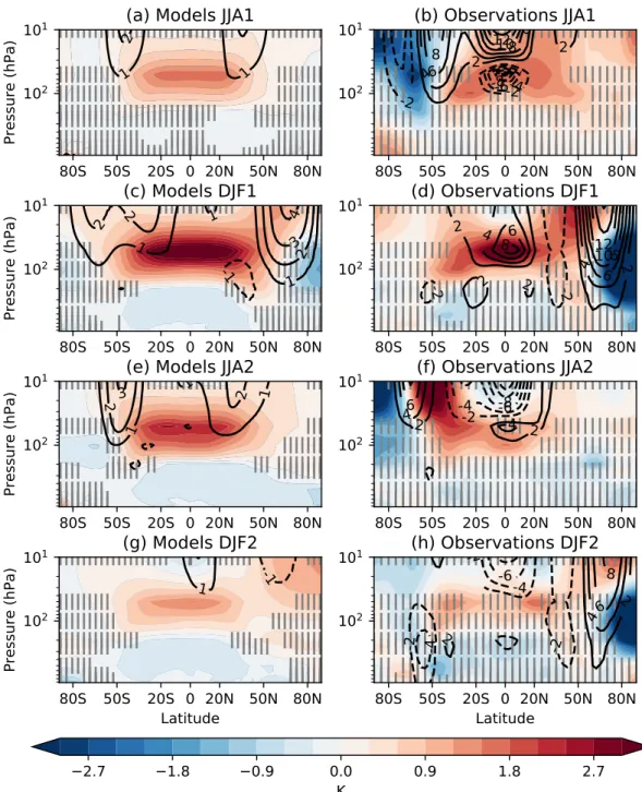
Figure 2 shows the zonal-mean temperature in the atmosphere throughout the first 2 years after the erup-tion for the June-July-August (JJA, boreal summer) and December-January-February (DJF, boreal winter)
Figure 2. Zonal-mean cross sections in the atmosphere of temperature anomalies (shaded) and zonal wind anomalies (contours, m/s) for the first and second December-January-February (DJF) and June-July-August (JJA) seasons after the eruptions for the multimodel ensemble mean (a, c, e, g) and an average of reanalyses (b, d, f, h). Values not
significant (p> 0.05) for temperature are hatched.
seasons. In general, the most of the lower stratosphere warms and the troposphere cools (particularly in the tropics). The warming in the models and the observations is similar in magnitude, but the tropospheric cooling is patchier and not significant in the observations.
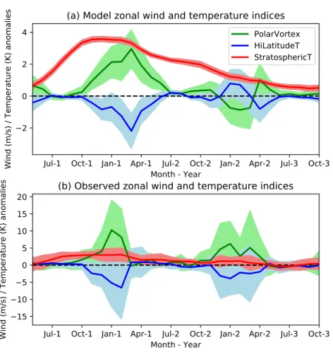
Figure 3a shows a time series of the stratospheric warming in the models (red line) defined as the average temperature at 50 hPa between 30◦S and 30◦N. The peak warming in the stratosphere happens about 7 to 9 months after the eruptions (around the first DJF, DJF1). It then reduces over the next year as the amount of volcanic aerosol declines in the stratosphere. The red line in Figure 3b shows the equivalent time series
Journal of Geophysical Research: Atmospheres
10.1029/2019JD031739
Figure 3. Zonal wind and temperature anomalies for the multimodel ensemble (a) and observations (b) with 90% confidence intervals. Polar vortex anomalies (PolarVortex, green) are the average zonal velocity over 50–100 hPa and
55◦N–75◦N, high-latitude upper-troposphere temperature (HiLatitudeT, blue) is the average temperature over 50–200
hPa and 70◦N–90◦N, and stratospheric temperature (StratosphericT, red) is the average temperature at 50 hPa
between 30◦S and 30◦N. Note that the vertical axis scale is different between (a) and (b).
for the observations. Note that the vertical axis has changed between panels (a) and (b). The timing and magnitude of the stratospheric warming is close between models and observations.
The time evolution in the models of the polar vortex anomalies defined as the average zonal velocity over 50–100 hPa and 55◦N–75◦N is shown by the green line in Figure 3a. The anomalies increase in magnitude in the boreal autumn and peak in late boreal winter in the first year after the eruption. The polar vortex does not exist in boreal summer, but the second DJF (DJF2), the tropical stratospheric heating is a third of what it was in the first winter, and there are no significant anomalies in the polar vortex. The green line in Figure 3b shows that polar vortex on average strengthens much more in the observations than in the models. The zonal-mean zonal winds (black contour lines) show the strongest response in DJF1, Figures 2c and 2d, when the stratospheric warming is the strongest. Even though the stratospheric warming is similar between models and the observations, the response of the wind is stronger in the observations (the polar vortex anomalies for DJF1 in the models and observations are both significantly different from zero, and they are significantly different from each other, defined as that the bootstrapped 90% confidence intervals around the two means do not overlap). The observations are about three times stronger than the models (the range is between 2.5 and 6 times stronger when taking the uncertainty of the model mean into account). It appears from Figures 2c and 2d that the northern edge of the midlatitude tropospheric jet is weakened in DJF1. The latitude of the jet changes with longitude, so the zonal-mean value is misleading. In the Atlantic, the jet is split into two: The midlatitude jet is shifted North, while the subtropical jet is strengthened. In the Pacific, the jet is shifted South (see in supporting information Figure S1).
Figure 4. Mean sea-level pressure anomalies for the first (a, b) and second DJF (c, d) after the eruptions for the multimodel ensemble mean (a, c) and an average of reanalyses (b, d). Note that the color scales are different between models and observations. Significant values are stippled.
Also notable in Figures 2c, 2d, and 2h are the cold temperature anomalies at high latitudes in boreal winter. In DJF1, like the zonal winds, the cooling anomaly is much weaker in models compared to observations. The time series of the cooling in the Northern Hemisphere defined as the average temperature over 50–200 hPa and 70◦N–90◦N is shown in Figure 3 as the blue line. For both models and observations, it is anticorrelated with the polar vortex. This implies that the upper-troposphere cold anomalies over the Arctic are probably caused by the strengthened polar vortex through cooling as air rises (Limpasuvan et al., 2005).
In DJF2, Figures 2g and 2h, models show a weak decrease in the polar vortex, while in observations, the response is similar to DJF1, although it is weaker (the polar vortex anomaly for observations is significantly different from zero and significantly different from the models, the polar vortex response for the models is not significantly different from zero). Associated with this, the upper-troposphere Arctic temperatures are anomalously cold in the observations, but there is no significant anomaly in the models.
3.2. Surface Responses
The Northern Hemisphere circulation changes in the mean sea-level pressure in the two winters following the eruptions are shown in Figure 4. In DJF1, panels (a) and (b), there is a low over the Arctic and a high over Europe for both models and observations. Driscoll et al. (2012) found that the response in CMIP5 models was about 10 times weaker than in observations. We find a similar result here, the model anomalies are about seven times weaker than the observational anomalies in the Atlantic region. We have used a different range of contours for models and observations in Figure 4 so that patterns can be compared even if the magnitudes are different. As found above, in DJF2, observations have a similar response to DJF1, compare panels (b) and (d). The response in the models, shown in panel (c), is different and is dominated by a low pressure in the Northeast Atlantic.
Journal of Geophysical Research: Atmospheres
10.1029/2019JD031739
Figure 5. Surface temperature anomalies for the first (a, b) and second DJF (c, d) after the eruptions for the multimodel ensemble mean (a, c) and an average of reanalyses (b, d). Significant values are stippled.
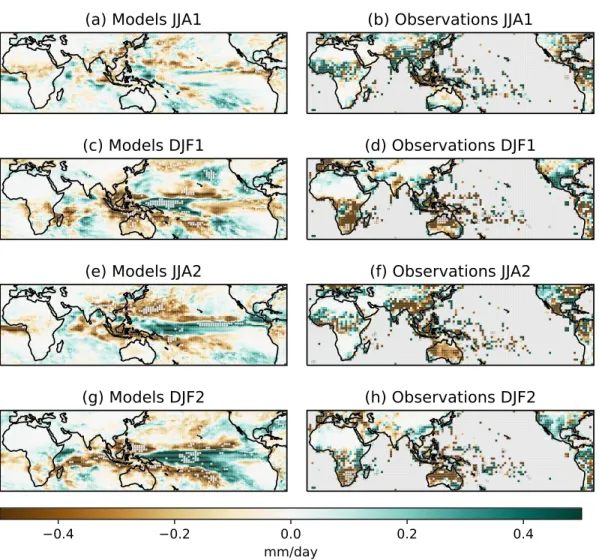
This circulation change in DJF1 has an impact on Northern Hemisphere winter surface temperatures, shown in Figures 5a and 5b. While in DJF1, the tropics have cooled (especially over land), both the mod-els and the observations show warm anomalies over Scandinavia and northern Russia (though this is not significant for the models). Again, model anomalies are weaker than in the observations for the surface tem-perature, presumably due the weaker circulation response. In DJF1 and DJF2, the cooling appears more uniform in the models than in the observations, though this may be because we are comparing an ensem-ble mean with an average of three volcanoes, which would have more noise. As discussed above, the global mean surface temperature response is not significantly different between the observations and the models. Tropical precipitation, shown in Figure 6, has anomalies over equatorial Africa already in JJA1 (panels a and b), though they are not significant. This is the largest equatorial land mass, and as it cools faster than the surrounding oceans, this might cause the reduction in precipitation (Khodri et al., 2017). The main feature of the precipitation, for which there is good agreement between models and observations, especially after JJA1, is that precipitation is reduced over the maritime continent. In DJF1 (panel c), the models show positive precipitation anomalies in the equatorial West Pacific. This is maintained for the next year as the precipitation anomalies spread East (panels e and g). There are dry anomalies in Australia in DJF1 (panels c and d) and in Southeast Asia in JJA2 (panels e and f) that suggest the monsoons there are reduced as was found by several studies, for example, Iles et al. (2013), Iles and Hegerl (2014), Liu et al. (2016), and Paik and Min (2018).
3.3. Impact on ENSO
The precipitation in Figure 6 shows, at least for the models, indications of the growth of an El Niño-like state from JJA1 to DJF2. Precipitation reduces over the Maritime Continent and increases to the East in the first year after the eruption. This increase in precipitation then spreads eastwards over the following year. For DJF2, the temperatures of Figure 5c in the central equatorial Pacific show no cooling in contrast to most of the rest of the tropics.
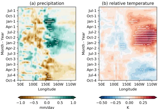
To see this more clearly, Figure 7 shows Hovmöller plots of monthly mean model precipitation and temper-ature anomalies in the equatorial Indo-Pacific. After about 8 months, around January of the first year after the eruptions, a clear dipole emerges in the precipitation, indicating that it has shifted East. In the following year, it spreads further East. As surface temperatures are dominated by the tropical cooling, in Figure 7b, we
Figure 6. Precipitation anomalies (mm/day) for the first and second DJF and JJA after the eruptions for the multimodel ensemble mean (a, c, e, g) and observations (b, d, f, h). Significant values are stippled. Note that observations do not exist over the ocean (gray).
show the surface temperature relative to the whole of the tropics (20◦S–20◦N). This shows eastward prop-agation of anomalies from about a year after the eruption, peaking in the second October after the eruption, similar to an El Niño.
Figure 8 shows relative sea surface temperature (RSST), the temperature difference between the NINO3.4 region and the tropical average (20◦S–20◦N) as used by Khodri et al. (2017). For the models, RSST is positive for the first 2 years after the eruptions and peaks in the second October. The observed average is also positive or stays close to zero. The uncertainties around the observed values are large, and the confidence interval never excludes zero but also includes the model ensemble.
Sensitivity studies by Khodri et al. (2017) in the atmospheric component of the Institute Pierre Simon Laplace-Coupled Model (IPSL-CM5B, not part of this study) showed that the chain of events leading to an El Niño-like response to volcanic aerosols in the second year started with reduced African precipita-tion. Figure 6a shows precipitation anomalies of the right sign over Africa in JJA1 (for models only), and Figure 7a shows propagation eastward in the Indian Ocean following this (not significant). So while we cannot exclude Africa being an important initiator of the mechanism, the strongest signals appear over the Maritime Continent about 6 months after the eruptions.
The results here are consistent with Ohba et al. (2013) and Predybaylo et al. (2017) who find that the Mar-itime Continent is important for the ENSO response. It is the relatively stronger cooling here compared to the tropical West Pacific that likely causes the precipitation to move to the tropical West Pacific. The sea
Journal of Geophysical Research: Atmospheres
10.1029/2019JD031739
Figure 7. Indo-Pacific equatorial (5◦S–5◦N) multimodel ensemble mean Hovmöller plots for (a) precipitation
(mm/day) and (b) surface temperature relative to the tropics (20◦S–20◦N, K). Stippling indicates significant values.
surface temperature (SST) in the central and East Pacific is controlled by upwelling and so cools less than the West Pacific. This weakens the easterly trade winds, which increases the SSTs in the East Pacific further through the Bjerknes feedback, leading to an El Niño response (Predybaylo et al., 2017).
Despite the lack of a detectable El Niño in observations, the precipitation fields in Figure 6h for observations in DJF2 show many known teleconnections to El Niño: low precipitation in Southern Africa, Australia, and the Maritime Continent as well as increased precipitation in Southern United States. Stevenson et al. (2016)
Figure 8. Surface temperature relative to the tropics in the NINO3.4 region for the multimodel ensemble (blue) and observations (black). The shaded areas around the time series represent the 90% confidence intervals found from a bootstrap with replacement.
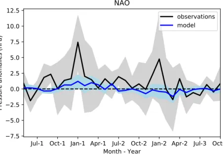
Figure 9. NAO index for the multimodel ensemble (blue) and observations (black). The shaded areas around the time series represent the 90% confidence intervals found from a bootstrap with replacement.
found that circulation changes due to volcanic eruptions can lead to precipitation anomalies that are similar to those associated with El Niño even when there is no ENSO event in surface temperatures.
3.4. Impact on the NAO
We now look closer at the climate response over the Atlantic sector. Figure 9 shows the model NAO index and observed NAO. The NAO is defined as the difference, south minus north, in mean sea-level pressure between two large boxes bounded by the longitudes 90◦W–60◦E. The northern box is bounded by 55◦N–90◦ N and the southern box by 20◦N–55◦N as in Stephenson et al. (2006). The boxes are shown in Figure 4a and are chosen to be large so that the exact location of the NAO in the different models is not important. The NAO indices in the model and observations are both positive in the first winter after the eruption, but as expected from Figures 4a and 4b, the amplitude is about seven times stronger in the observations than in the models (note that the 90% confidence intervals do not overlap between models and observations for the first January). In the second winter, the response is not significant as the confidence intervals for the observed NAO and modeled NAO both include zero.
Comparing the NAO (Figure 9) with the indices in Figure 3 supports that the NAO response in DJF1 is related to the stratospheric tropical warming via the polar vortex. The warming increases the stratospheric temperature gradient between 40◦N and the pole. This strengthens the polar vortex (Stenchikov et al., 2002; Shindell et al., 2004; Driscoll et al., 2012; Swingedouw et al., 2017). In addition, increasing extratropical west-erly wind anomalies (Figures 2c and 2d) increase propagation of planetary waves into the tropics and hence reduce the wave flux into the vortex, further stabilizing and strengthening it (Bittner et al., 2016), though this has not been analyzed here. The lag between the tropical stratospheric warming and the strengthening of the polar vortex at the beginning of the time series in Figure 3 is likely because the polar vortex only exists in winter.
The tropical stratospheric warming has been questioned as a mechanism (Swingedouw et al., 2017) as in the stratosphere, the tropics are colder than the polar region. This would mean that warming the tropical stratosphere would decrease the meridional temperature gradient, not increase it. However, in the models used here, we find in DJF1 that there is a climatological temperature maximum (found by averaging all DJF1 of the experiments without volcanic aerosols) at 40◦N at the 50- and 100-hPa levels, so the warming does indeed increase the temperature gradient. This climatological maximum exists in the observations as well, so this is a realistic response.
3.5. Impact on the North Atlantic Ocean
To explore the potential longer-term climate response (though the experiments only continue for 4 years after the volcanic eruption), we look at the North Atlantic Ocean, a region where volcanoes can induce
Journal of Geophysical Research: Atmospheres
10.1029/2019JD031739
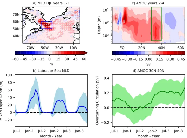
Figure 10. North Atlantic dynamic impacts. (a) Multimodel ensemble mean mixed layer depth (MLD) anomaly averaged over the first three winters (DJF) following the volcanic eruptions and (b) averaged monthly MLD anomaly over the Labrador Sea (blue box in panel a). (c) Multimodel ensemble mean Atlantic Meridional Overturning Circulation (AMOC) streamfunction anomaly averaged over Years 2–4 after the eruptions and (d) averaged AMOC streamfunction anomaly (green box in panel c). A 12-month running mean has been applied to this time series to focus on the interannual variability.
changes at decadal timescales (Ding et al., 2014; Mignot et al., 2011; Stenchikov et al., 2009; Swingedouw et al., 2017). Figure 10a shows an anomalously deep mixed layer (which can be interpreted as a proxy for deep convection) during the three boreal winters following the eruptions, with a maximum in the Labrador Sea. The time series averaged over the blue box can be seen in Figure 10b. It shows that the ensemble with volcanic aerosols included has a deeper mixed layer than the ensemble without volcanic aerosols in late boreal winter and spring for the first 2 years after the eruptions. A strengthened NAO, as seen in Figure 9 for the first winter and early spring, would favor downwelling from Ekman pumping south of the strengthened winds (where there is negative wind stress curl), leading to the increased mixed layer depth (MLD) seen in Figure 10 for the first winter.
Figure 10c shows the AMOC streamfunction anomaly for Years 2–4 after the volcanic eruption. A barotropic response can be seen, strongest between 30◦N and 40◦N, which strengthens the circulation. Although the anomaly is not significant over this period, this is in line with previous literature identifying similar AMOC intensifications in different models, which are caused by either a rapid dynamical adjustment related to a dominant negative wind stress curl anomaly over the subpolar North Atlantic forced by the eruptions (Mignot et al., 2011; Zanchettin et al., 2012) or enhanced deep convection activity in response to the surface cooling, salinification (due to reduced precipitation), and subsequent weakening of density stratification in the Labrador Sea (Iwi et al., 2012; Ortega et al., 2012; Stenchikov et al., 2009). There is a significant response in the streamfunction over the equator, which is caused by anomalous easterly winds.
A smoothed time series of the AMOC from the green box on Figure 10c is shown in Figure 10d. The response of the AMOC to the deepened MLD typically has a lag of 2–3 years between a peak in convection and the AMOC (Eden & Willebrand, 2001; Ortega et al., 2017), which is consistent with Figure 10d. As the positive
NAO signal weakens after the first winter, the response to surface cooling and salinification is likely to become more important in driving the AMOC anomalies thereafter (Stenchikov et al., 2009).
4. Conclusions
In this multimodel study with initialized climate prediction systems, we have used an experimental design created specifically to clarify the impact of volcanic aerosols on near-term climate and reduce model biases (Boer et al., 2016): Anomalies are the difference between an ensemble that includes volcanic aerosols and one without volcanic aerosols. Both ensembles include all other external forcings relevant to the time of the eruptions. We combine three different volcanic eruptions, Agung, El Chichón, and Pinatubo, to get a total ensemble size of 135 members with volcanic aerosols and 128 without.
Global temperature cools, peaking at about −0.2 K a year after the eruptions in both models and observations (Figure 1), though uncertainties are large in the observations. We find that the models simulate realistic levels of warming in the stratosphere (Figure 2), but zonal-mean winds in the first winter are approximately three times weaker than in observations (cf. Figures 2c and 2d). At the surface, both mean sea-level pressure (Figures 4a and 4b) and temperature (Figures 5a and 5b) show similar patterns to observations in the first winter, but the modeled amplitude is about seven times weaker. We are not claiming that models cannot display zonal winds, temperatures, and sea-level pressures of the observed magnitude, but since the model response is weak in the ensemble mean (which is a measure of the signal, after the noise has been averaged out), then either the response is spurious in the observations or the response is too weak in the models. Comparison with observations is difficult as they are noisy, and we are only considering a few cases, but this makes the similarity in patterns between models and observations all the more surprising and implies that the observed signal is stronger than previously thought. The case for the response being too weak in the models is strengthened by the fact that many recent studies have found that patterns in supposedly noisy observations are reproduced in models, but with reduced magnitude, especially around the North Atlantic (Baker et al., 2018; Dunstone et al., 2016; Scaife & Smith, 2018; Siegert et al., 2016; Smith et al., 2019). In the second winter, observations show a persistence of the same pattern as the first winter, but it is weaker and less significant. This persistence is not simulated by the models.
An El Niño-like state, which develops in the models about 1 year after the eruptions, grows to a maxi-mum around the second winter (Figure 7). This is initiated by an eastward shift in precipitation from the Maritime Continent toward the western tropical Pacific that starts within a few months of the eruptions (Figures 6a and 6b). This could be related to the Maritime Continent cooling faster under the influence of volcanic aerosols than the surrounding oceans. This robust impact on ENSO in the models is not visible in the observations, possibly due to the large amount of noise present (Figure 8).
Models and observations both have a positive NAO-like pattern in the first winter after the eruptions (Figures 4a and 4b), in agreement with some previous studies (Shindell et al., 2004; Stenchikov et al., 2002; Zambri & Robock, 2016). The positive NAO is likely caused by a strengthened polar vortex driven by the warming in the lower tropical stratosphere (Figure 3). The amplitude of the NAO anomaly is about seven times weaker in the models than in the observations in the first winter (Figure 9). The signal-to-noise ratio appears to be too small in the models, consistent with other studies (Baker et al., 2018; Dunstone et al., 2016; Eade et al., 2014; Scaife & Smith, 2018). In the second winter, neither the observations nor the models have a significant NAO signal, though the observed mean sea-level pattern is NAO-like (Figure 4d).
Finally, we find dynamical changes in the Atlantic Ocean (Figure 10). Even for the short length of these experiments (4 years), there is already a strengthening of the AMOC. This is probably mediated by changes in wind stress curl and increased MLDs. The volcanic response therefore likely extends beyond the length of these experiments, potentially leading to a positive phase of the Atlantic Multidecadal Variability (AMV, Knight et al., 2005; Ottera et al., 2010) and increases to the ocean heat content in the subpolar North Atlantic (Hermanson et al., 2014; Robson et al., 2012), with important impacts over land (Hermanson et al., 2014; Robson et al., 2013).
References
Adams, J. B., Mann, M. E., & Ammann, C. M. (2003). Proxy evidence for an El Niño-like response to volcanic forcing. Nature, 426, 274–278. https://doi.org/10.1038/nature02101
Acknowledgments
We thank the three reviewers for their help in improving this manuscript. The data are available from DOI (10.5281/zenodo.2613699). L. H. was supported by the Climate Resilience Project funded by UKRI. N. D. and D. M. S. were supported by the Met Office Hadley Centre Climate Programme funded by BEIS and Defra. M. M., R. B., and P. O. received funding from the Ministerio de Economia y
Competitividad (MINECO) as part of the VOLCADEC (Ref.
CGL2015-70177-R) and HIATUS (Ref. CGL2015-70353-R) projects. H. P. and C. T. were supported by the German Ministry of Education and Research (BMBF) under the project MiKlip (Grants 01LP1519A and 01LP1517B). J. I. R. was supported by the Natural Environmental Research Council (NERC)-funded SMURPHS project and the ACSIS program. HiGEM-DP experiments were performed using the ARCHER UK National
Supercomputing Service (http://www. archer.ac.uk). The National Center for Atmospheric Research (NCAR) is a major facility sponsored by the U.S. National Science Foundation (NSF) under Cooperative Agreement No. 1852977. G. D. and S. Y. further acknowledge the support of NSF Collaborative Research EaSM2 Grant OCE-1243015. G. S. was supported by the Regional and Global Climate Modeling Program (RGCM) of the U.S. Department of Energy's, Office of Science (BER), Cooperative Agreement DE-FC02-97ER62402.
Journal of Geophysical Research: Atmospheres
10.1029/2019JD031739
Ammann, C. M., Meehl, G. A., Washington, W. M., & Zender, C. S. (2003). A monthly and latitudinally varying volcanic forcing dataset in simulations of 20th century climate. Geophysical Research Letters, 30(12), 1657. https://doi.org/10.1029/2003GL016875
Baker, L. H., Shaffrey, L. C., Sutton, R. T., Weisheimer, A., & Scaife, A. A. (2018). An intercomparison of skill and overconfi-dence/underconfidence of the wintertime North Atlantic Oscillation in multimodel seasonal forecasts. Geophysical Research Letters, 45, 7808–7817. https://doi.org/10.1029/2018GL078838
Barnes, E. A., Solomon, S., & Polvani, L. M. (2016). Robust wind and precipitation responses to the Mount Pinatubo eruption, as simulated in the CMIP5 models. Journal of Climate, 29(13), 4763–4778. https://doi.org/10.1175/JCLI-D-15-0658.1
Bittner, M., Schmidt, H., Timmreck, C., & Sienz, F. (2016). Using a large ensemble of simulations to assess the Northern Hemisphere stratospheric dynamical response to tropical volcanic eruptions and its uncertainty. Geophysical Research Letters, 43, 9324–9332. https:// doi.org/10.1002/2016GL070587
Bittner, M., Timmreck, C., Schmidt, H., Toohey, M., & Krüger, K. (2016). The impact of wave-mean flow interaction on the Northern Hemisphere polar vortex after tropical volcanic eruptions. Journal of Geophysical Research: Atmospheres, 121, 5281–5297. https://doi. org/10.1002/2015JD024603
Boer, G. J., Smith, D. M., Cassou, C., Doblas-Reyes, F., Danabasoglu, G., Kirtman, B., et al. (2016). The Decadal Climate Prediction Project (DCPP) contribution to CMIP6. Geoscientific Model Development, 9(10), 3751–3777. https://doi.org/10.5194/gmd-9-3751-2016 Clark, R. T., Bett, P. E., Thornton, H. E., & Scaife, A. A. (2017). Skilful seasonal predictions for the European energy industry. Environmental
Research Letters, 12(2), 24,002. https://doi.org/10.1088/1748-9326/aa57ab
Ding, Y., Carton, J. A., Chepurin, G. A., Stenchikov, G., Robock, A., Sentman, L. T., & Krasting, J. P. (2014). Ocean response to volcanic eruptions in Coupled Model Intercomparison Project 5 simulations. Journal of Geophysical Research: Oceans, 119, 5622–5637. https:// doi.org/10.1002/2013JC009780
Driscoll, S., Bozzo, A., Gray, L. J., Robock, A., & Stenchikov, G. (2012). Coupled Model Intercomparison Project 5 (CMIP5) simulations of climate following volcanic eruptions. Journal of Geophysical Research, 117, D17105. https://doi.org/10.1029/2012JD017607
Dunstone, N. D., Smith, D. M., Scaife, A. A., Hermanson, L., Eade, R., Robinson, N., et al. (2016). Skilful predictions of the winter North Atlantic Oscillation one year ahead. Nature Geosciences, 9, 809–814. https://doi.org/10.1038/ngeo2824
Eade, R., Smith, D., Scaife, A., Wallace, E., Dunstone, N., Hermanson, L., & Robinson, N. (2014). Do seasonal-to-decadal climate predictions underestimate the predictability of the real world? Geophysical Research Letters, 41, 5620–5628. https://doi.org/10.1002/2014GL061146 Eden, C., & Willebrand, J. (2001). Mechanism of interannual to decadal variability of the North Atlantic circulation. Journal of Climate,
14(10), 2266–2280. https://doi.org/10.1175/1520-0442(2001)014<2266:MOITDV>2.0.CO;2
Giorgetta, M. A., Jungclaus, J., Reick, C. H., Legutke, S., Bader, J., Buttinger, M., et al. (2013). Climate and carbon cycle changes from 1850 to 2100 in MPI-ESM simulations for the Coupled Model Intercomparison Project phase 5. Journal of Advances in Modeling Earth
Systems, 5, 572–597. https://doi.org/10.1002/jame.20038
Hansen, J., Ruedy, R., Sato, M., & Lo, K. (2010). Global surface temperature change. Reviews of Geophysics, 48, RG4004. https://doi.org/10. 1029/2010RG000345
Hansen, J., Sato, M., & Ruedy, R. (1997). Radiative forcing and climate response. Journal of Geophysical Research, 102, 6831–6864. Harada, Y., Kamahori, H., Kobayashi, C., Endo, H., Kobayashi, S., Ota, Y., et al. (2016). The JRA-55 reanalysis: Representation of
atmospheric circulation and climate variability. Journal of the Meteorological Society of Japan. Series II, 94(3), 269–302. https://doi.org/ 10.2151/jmsj.2016-015
Hazeleger, W., Wang, X., Severijns, C., ¸Stef˘anescu, S., Bintanja, R., Sterl, A., et al. (2012). EC-Earth V2.2: Description and validation of a new seamless earth system prediction model. Climate Dynamics, 39(11), 2611–2629. https://doi.org/10.1007/s00382-011-1228-5 Hermanson, L., Eade, R., Robinson, N. H., Dunstone, N. J., Andrews, M. B., Knight, J. R., et al. (2014). Forecast cooling of the Atlantic
subpolar gyre and associated impacts. Geophysical Research Letters, 41, 5167–5174. https://doi.org/10.1002/2014GL060420
Hurrell, J. W., Holland, M. M., Gent, P. R., Ghan, S., Kay, J. E., Kushner, P. J., et al. (2013). The Community Earth System Model: A framework for collaborative research. Bulletin of the American Meteorological Society, 94(9), 1339–1360. https://doi.org/10.1175/ BAMS-D-12-00121.1
Iles, C. E., & Hegerl, G. C. (2014). The global precipitation response to volcanic eruptions in the CMIP5 models. Environmental Research
Letters, 9(10), 104,012. https://doi.org/10.1088/1748-9326/9/10/104012
Iles, C. E., Hegerl, G. C., Schurer, A. P., & Zhang, X. (2013). The effect of volcanic eruptions on global precipitation. Journal of Geophysical
Research: Atmospheres, 118, 8770–8786. https://doi.org/10.1002/jgrd.50678
Illing, S., Kadow, C., Pohlmann, H., & Timmreck, C. (2018). Assessing the impact of a future volcanic eruption on decadal predictions.
Earth System Dynamics, 9(2), 701–715. https://doi.org/10.5194/esd-9-701-2018
Iwi, A. M., Hermanson, L., Haines, K., & Sutton, R. T. (2012). Mechanisms linking volcanic aerosols to the Atlantic Meridional Overturning Circulation. Journal of Climate, 25(8), 3039–3051. https://doi.org/10.1175/2011JCLI4067.1
Kalnay, E., Kanamitsu, M., Kistler, R., Collins, W., Deaven, D., Gandin, L., et al. (1996). The NCEP/NCAR 40-year reanalysis project.
Bulletin of the American Meteorological Society, 77(3), 437–472. https://doi.org/10.1175/1520-0477(1996)077<0437:TNYRP>2.0.CO;2 Karl, T. R., Arguez, A., Huang, B., Lawrimore, J. H., McMahon, J. R., Menne, M. J., et al. (2015). Possible artifacts of data biases in the
recent global surface warming hiatus. Science, 348(6242), 1469–1472. https://doi.org/10.1126/science.aaa5632
Khodri, M., Izumo, T., Vialard, J., Janicot, S., Cassou, C., Lengaigne, M., et al. (2017). Tropical explosive volcanic eruptions can trigger El Niño by cooling tropical Africa. Nature Communications, 8, 778. https://doi.org/10.1038/s41467-017-00755-6
Knight, J. R., Allan, R. J., Folland, C. K., Vellinga, M., & Mann, M. E. (2005). A signature of persistent natural thermohaline circulation cycles in observed climate. Geophysical Research Letters, 33, L20708. https://doi.org/10.1029/2005GL024233
Lacis, A., Hansen, J., & Sato, M. (1992). Climate forcing by stratospheric aerosols. Geophysical Research Letters, 19, 1607–1610. Lehner, F., Schurer, A. P., Hegerl, G. C., Deser, C., & Frölicher, T. L. (2016). The importance of ENSO phase during volcanic eruptions for
detection and attribution. Geophysical Research Letters, 43, 2851–2858. https://doi.org/10.1002/2016GL067935
Limpasuvan, V., Hartmann, D. L., Thompson, D. W. J., Jeev, K., & Yung, Y. L. (2005). Stratosphere-troposphere evolution during polar vortex intensification. Journal of Geophysical Research, 110, D24101. https://doi.org/10.1029/2005JD006302
Liu, F., Chai, J., Wang, B., Liu, J., Zhang, X., & Wang, Z. (2016). Global monsoon precipitation responses to large volcanic eruptions.
Scientific Reports, 6, 24,331. https://doi.org/10.1038/srep24331
Ménégoz, M., Bilbao, R., Bellprat, O., Guemas, V., & Doblas-Reyes, F. J. (2018). Forecasting the climate response to volcanic eruptions: Prediction skill related to stratospheric aerosol forcing. Environmental Research Letters, 13(6), 64,022. https://doi.org/10.1088/1748-9326/ aac4db
Ménégoz, M., Cassou, C., Swingedouw, D., Ruprich-Robert, Y., Bretonnière, P.-A., & Doblas-Reyes, F. (2018). Role of the Atlantic Multi-decadal Variability in modulating the climate response to a Pinatubo-like volcanic eruption. Climate Dynamics, 51(5), 1863–1883. https:// doi.org/10.1007/s00382-017-3986-1
Maher, N., McGregor, S., England, M. H., & Gupta, A. S. (2015). Effects of volcanism on tropical variability. Geophysical Research Letters,
42, 6024–6033. https://doi.org/10.1002/2015GL064751
Mignot, J., Khodri, M., Frankignoul, C., & Servonnat, J. (2011). Volcanic impact on the Atlantic Ocean over the last millennium. Climate
of the Past, 7(4), 1439–1455. https://doi.org/10.5194/cp-7-1439-2011
Morice, C. P., Kennedy, J. J., Rayner, N. A., & Jones, P. D. (2012). Quantifying uncertainties in global and regional temperature change using an ensemble of observational estimates: The HadCRUT4 data set. Journal of Geophysical Research, 117, D08101. https://doi.org/ 10.1029/2011JD017187
Ohba, M., Shiogama, H., Yokohata, T., & Watanabe, M. (2013). Impact of strong tropical volcanic eruptions on ENSO simulated in a coupled GCM. Journal of Climate, 26(14), 5169–5182. https://doi.org/10.1175/JCLI-D-12-00471.1
Ortega, P., Montoya, M., González-Rouco, F., Mignot, J., & Legutke, S. (2012). Variability of the Atlantic meridional overturning circulation in the last millennium and two IPCC scenarios. Climate Dynamics, 38(9), 1925–1947. https://doi.org/10.1007/s00382-011-1081-6 Ortega, P., Robson, J., Sutton, R. T., & Andrews, M. B. (2017). Mechanisms of decadal variability in the Labrador Sea and the wider north
atlantic in a high-resolution climate model. Climate Dynamics, 49(7), 2625–2647. https://doi.org/10.1007/s00382-016-3467-y Ottera, O. H., Bentsen, M., Drange, H., & Suo, L. (2010). External forcing as a metronome for Atlantic multidecadal variability. Nature
Geoscience, 3, 688–694.
Paik, S., & Min, S.-K. (2018). Assessing the impact of volcanic eruptions on climate extremes using CMIP5 models. Journal of Climate,
31(14), 5333–5349. https://doi.org/10.1175/JCLI-D-17-0651.1
Pohlmann, H., Müller, W. A., Kulkarni, K., Kameswarrao, M., Matei, D., Vamborg, F. S. E., et al. (2013). Improved forecast skill in the tropics in the new MiKlip decadal climate predictions. Geophysical Research Letters, 40, 5798–5802. https://doi.org/10.1002/2013GL058051 Predybaylo, E., Stenchikov, G. L., Wittenberg, A. T., & Zeng, F. (2017). Impacts of a Pinatubo-size volcanic eruption on ENSO. Journal of
Geophysical Research: Atmospheres, 122, 925–947. https://doi.org/10.1002/2016JD025796
Robock, A. (2000). Volcanic eruptions and climate. Reviews of Geophysics, 38(2), 191–219. https://doi.org/10.1029/1998RG000054 Robock, A., & Mao, J. (1992). Winter warming from large volcanic eruptions. Geophysical Research Letters, 19(24), 2405–2408. https://doi.
org/10.1029/92GL02627
Robson, J., Polo, I., Hodson, D. L. R., Stevens, D. P., & Shaffrey, L. C. (2018). Decadal prediction of the North Atlantic subpolar gyre in the HiGEM high-resolution climate model. Climate Dynamics, 50(3), 921–937. https://doi.org/10.1007/s00382-017-3649-2
Robson, J. I., Sutton, R. T., Lohmann, K., Smith, D. M., & Palmer, M. D. (2012). Causes of the rapid warming of the North Atlantic Ocean in the mid-1990s. Journal of Climate, 25, 4116–4134. https://doi.org/10.1175/JCLI-D-11-00443.1
Robson, J., Sutton, R., & Smith, D. (2013). Predictable climate impacts of the decadal changes in the ocean in the 1990s. Journal of Climate,
26(17), 6329–6339. https://doi.org/10.1175/JCLI-D-12-00827.1
Sato, M., Hansen, J. E., McCormick, M. P., & Pollack, J. B. (1993). Stratospheric aerosol optical depths, 1850–1990. Journal of Geophysical
Research, 98(D12), 22,987–22,994. https://doi.org/10.1029/93JD02553
Scaife, A. A., & Smith, D. (2018). A signal-to-noise paradox in climate science. npj Climate and Atmospheric Science, 1(28), 9031–9041. https://doi.org/10.1038/s41612-018-0038-4
Schneider, U., Becker, A., Finger, P., Meyer-Christoffer, A., Ziese, M., & Rudolf, B. (2014). GPCC's new land surface precipitation clima-tology based on quality-controlled in situ data and its role in quantifying the global water cycle. Theoretical and Applied Climaclima-tology,
115(1), 15–40. https://doi.org/10.1007/s00704-013-0860-x
Shaffrey, L. C., Stevens, I., Norton, W. A., Roberts, M. J., Vidale, P. L., Harle, J. D., et al. (2009). U.K. HiGEM: The new U.K. High-Resolution Global Environment Model: Model description and basic evaluation. Journal of Climate, 22(8), 1861–1896. https://doi.org/10.1175/ 2008JCLI2508.1
Shindell, D. T., Schmidt, G. A., Mann, M. E., & Faluvegi, G. (2004). Dynamic winter climate response to large tropical volcanic eruptions since 1600. Journal of Geophysical Research, 109, D05104. https://doi.org/10.1029/2003JD004151
Siegert, S., Stephenson, D. B., Sansom, P. G., Scaife, A. A., Eade, R., & Arribas, A. (2016). A Bayesian framework for verification and recalibration of ensemble forecasts: How uncertain is NAO predictability? Journal of Climate, 29(3), 995–1012. https://doi.org/10.1175/ JCLI-D-15-0196.1
Smith, D. M., Booth, B. B. B., Dunstone, N. J., Eade, R., Hermanson, L., Jones, G. S., et al. (2016). Role of volcanic and anthropogenic aerosols in the recent global surface warming slowdown. Nature Climate Change, 6, 936–940. https://doi.org/10.1038/nclimate3058 Smith, D. M., Eade, R., Scaife, A. A., Caron, L.-P., Danabasoglu, G., DelSole, T. M., et al. (2019). Robust skill of decadal climate predictions.
npj Climate and Atmospheric Science, 2:13. https://doi.org/10.1038/s41612-019-0071
Stenchikov, G., Delworth, T. L., Ramaswamy, V., Stouffer, R. J., Wittenberg, A., & Zeng, F. (2009). Volcanic signals in oceans. Journal of
Geophysical Research, 114, D16104. https://doi.org/10.1029/2008JD011673
Stenchikov, G., Hamilton, K., Stouffer, R. J., Robock, A., Ramaswamy, V., Santer, B., & Graf, H.-F. (2006). Arctic Oscillation response to vol-canic eruptions in the IPCC AR4 climate models. Journal of Geophysical Research, 111, D07107. https://doi.org/10.1029/2005JD006286 Stenchikov, G. L., Kirchner, I., Robock, A., Graf, H.-F., Antuña, J. C., Grainger, R. G., et al. (1998). Radiative forcing from the 1991 Mount
Pinatubo volcanic eruption. Journal of Geophysical Research, 103, 13,837–13,857. https://doi.org/10.1029/98JD00693
Stenchikov, G., Robock, A., Ramaswamy, V., Schwarzkopf, M. D., Hamilton, K., & Ramachandran, S. (2002). Arctic Oscillation response to the 1991 Mount Pinatubo eruption: Effects of volcanic aerosols and ozone depletion. Journal of Geophysical Research, 107, 4803. https:// doi.org/10.1029/2002JD002090
Stephenson, D. B., Pavan, V., Collins, M., Junge, M. M., Quadrelli, R., & Participating CMIP2 Modelling Groups (2006). North Atlantic Oscillation response to transient greenhouse gas forcing and the impact on European winter climate: A CMIP2 multi-model assessment.
Climate Dynamics, 27, 401–420. https://doi.org/10.1007/s00382-006-0140-x
Stevenson, S., Fasullo, J. T., Otto-Bliesner, B. L., Tomas, R. A., & Gao, C. (2017). Role of eruption season in reconciling model and proxy responses to tropical volcanism. Proceedings of the National Academy of Sciences, 114(8), 1822–1826. https://doi.org/10.1073/pnas. 1612505114
Stevenson, S., Otto-Bliesner, B., Fasullo, J., & Brady, E. (2016). “El Niño like” hydroclimate responses to last millennium volcanic eruptions.
Journal of Climate, 29(8), 2907–2921. https://doi.org/10.1175/JCLI-D-15-0239.1
Swingedouw, D., Mignot, J., Ortega, P., Guilyardi, E., Masson-Delmotte, V., Butler, P. G., et al. (2015). Bidecadal North Atlantic ocean circulation variability controlled by timing of volcanic eruptions. Nature Communications, 6, 6545. https://doi.org/10.1038/ncomms7545 Swingedouw, D., Mignot, J., Ortega, P., Khodri, M., Menegoz, M., Cassou, C., & Hanquiez, V. (2017). Impact of explosive volcanic eruptions
on the main climate variability modes. Global and Planetary Change, 150, 24–45. https://doi.org/10.1016/j.gloplacha.2017.01.006 Taylor, K. E., Stouffer, R. J., & Meehl, G. A. (2012). An overview of CMIP5 and the experiment design. Bulletin of the American Meteorological
Journal of Geophysical Research: Atmospheres
10.1029/2019JD031739
Timmreck, C. (2012). Modeling the climatic effects of large explosive volcanic eruptions. Wiley Interdisciplinary Reviews: Climate Change,
3(6), 545–564. https://doi.org/10.1002/wcc.192
Timmreck, C., Pohlmann, H., Illing, S., & Kadow, C. (2016). The impact of stratospheric volcanic aerosol on decadal-scale climate predictions. Geophysical Research Letters, 43, 834–842. https://doi.org/10.1002/2015GL067431
Uppala, S. M., Kallberg, P. W., Simmons, A. J., Andrae, U., Bechtold, V. D. C., Fiorino, M., et al. (2005). The ERA-40 re-analysis. Quarterly
Journal of the Royal Meteorological Society, 131(612), 2961–3012. https://doi.org/10.1256/qj.04.176
Williams, K. D., Harris, C. M., Bodas-Salcedo, A., Camp, J., Comer, R. E., Copsey, D., et al. (2015). The Met Office Global Coupled Model 2.0 (GC2) configuration. Geoscientific Model Development, 8(5), 1509–1524. https://doi.org/10.5194/gmd-8-1509-2015
Wilson, R., Cook, E., D'Arrigo, R., Riedwyl, N., Evans, M. N., Tudhope, A., & Allan, R. (2010). Reconstructing ENSO: The influence of method, proxy data, climate forcing and teleconnections. Journal of Quaternary Science, 25(1), 62–78. https://doi.org/10.1002/jqs.1297 Yeager, S. G., Danabasoglu, G., Rosenbloom, N. A., Strand, W., Bates, S. C., Meehl, G. A., et al. (2018). Predicting near-term changes in the
Earth system: A large ensemble of initialized decadal prediction simulations using the Community Earth System Model. Bulletin of the
American Meteorological Society, 99(9), 1867–1886. https://doi.org/10.1175/BAMS-D-17-0098.1
Zambri, B., & Robock, A. (2016). Winter warming and summer monsoon reduction after volcanic eruptions in Coupled Model Intercom-parison Project 5 (CMIP5) simulations. Geophysical Research Letters, 43, 10,920–10,928. https://doi.org/10.1002/2016GL070460 Zanchettin, D., Bothe, O., Graf, H. F., Lorenz, S. J., Luterbacher, J., Timmreck, C., & Jungclaus, J. H. (2013). Background conditions
influ-ence the decadal climate response to strong volcanic eruptions. Journal of Geophysical Research: Atmospheres, 118, 4090–4106. https:// doi.org/10.1002/jgrd.50229
Zanchettin, D., Timmreck, C., Graf, H.-F., Rubino, A., Lorenz, S., Lohmann, K., et al. (2012). Bi-decadal variability excited in the coupled ocean–atmosphere system by strong tropical volcanic eruptions. Climate Dynamics, 39(1), 419–444. https://doi.org/10.1007/ s00382-011-1167-1
Zhong, Y., Miller, G. H., Otto-Bliesner, B. L., Holland, M. M., Bailey, D. A., Schneider, D. P., & Geirsdottir, A. (2011). Centennial-scale climate change from decadally-paced explosive volcanism: A coupled sea ice-ocean mechanism. Climate Dynamics, 37(11), 2373–2387. https://doi.org/10.1007/s00382-010-0967-z