A coupled theory for diffusion of hydrogen and large elastic-plastic deformations of metals

elastic-plastic deformations of metals

by

Claudio V. Di Leo

S.B., Massachusetts Institute of Technology (2010)

Submitted to the Department of Mechanical Engineering

in partial fulfillment of the requirements for the degree of

Master of Science

at the

Massachusetts Institute of Technology

June 2012

ARCHIVES

MASSACHUSETTS INSTIfUTE OF TECHNOLOGY

JUN 28 2012

LIBRARIES

®

Massachusetts Institute of Technology 2012. All rights reserved.

Author ...

...

...

Department of Mechanical Engineering

May 5, 2012

Certified by.... .*.v. ...

...

Lallit Anand

Warren and Towneley Rohsenow Professor of Mechanical Engineering

Thesis Supervisor

A ccepted by ... .2..

David E. Hardt

Chairman, Department Committee on Graduate Students

A coupled theory for diffusion of hydrogen and large elastic-plastic deformations of metals

by

Claudio V. Di Leo

Submitted to the Department of Mechanical Engineering on May 5, 2012, in partial fulfillment of the

requirements for the degree of Master of Science

Abstract

A thermodynamically-consistent coupled-theory which accounts for diffusion of hydrogen, trapping of hydrogen, diffusion of heat, and large elastic-plastic deformations of metals is developed. Our theoretical framework places the widely-used notion of an "equilibrium" between hydrogen resid-ing in normal interstitial lattice sites and hydrogen trapped at microstructural defects, within a thermodynamically-consistent framework. The theory has been numerically implemented in a fi-nite element program. Using the numerical capability we study two important problems. First, we show the importance of using a prescribed chemical potential boundary condition in modeling the boundary between a metal system and a hydrogen atmosphere at a given partial pressure and temperature; specifically, we perform simulations using this boundary condition and compare our simulations to those in the published literature. Secondly, the effects of hydrogen on the plastic deformation of metals is studied through simulations of plane-strain tensile deformation and three-point bending of U-Notched specimens. Our simulations on the effects of hydrogen on three-three-point bending of U-notched specimens are shown to be in good qualitative agreement with published experiments.

Thesis Supervisor: Lallit Anand

Acknowledgments

First and foremost I would like to thank my advisor Professor Lallit Anand. I have been inspired by his precise and rigorous treatment of the field of solid mechanics and I will continue to draw upon the skills I have learned from him for many years to come.

My colleagues at the mechanics and materials group have provided me with invaluable knowl-edge and friendship. I would particularly like to thank Kaspar Loeffel, Dr. David Henann, and Dr. Shawn Chester for many fruitful discussions. Dr. Vikas Srivastava was my mentor as an undergraduate research assistant and inspired me to pursue further studies in graduate school, I owe a special debt of gratitude to him. Additionally, I would like to thank Ray Hardin for his help with various administrative issues.

I thank my family, especially my parents, for always making me strive to become a better man. Through example, they have taught me that there is nothing you can not achieve if you work hard. Finally, I thank my wife Lea, she gives meaning and purpose to all my efforts.

List of Figures 11 List of Tables 13 1 Introduction 15 2 Theoretical framework 19 2.1 Introduction . . . . 19 2.2 N otation . . . . 19 2.3 K inem atics . . . . 19 2.3.1 Standard kinematics . . . . 19 2.3.2 An additional microvariable eP . . . . 22 2.4 Frame-indifference . . . . 22

2.5 Development of the theory based on the principle of virtual power . . . . 23

2.5.1 Principle of virtual power . . . . 24

2.5.2 Frame-indifference of the internal power and its consequences . . . . 25

2.5.3 Macroscopic force balance . . . . 26

2.5.4 Microscopic force balances . . . . 27

2.6 Balance law for the diffusion of hydrogen . . . . 28

2.7 Balance of energy. Entropy imbalance. Free-energy imbalance . . . . 29

2.8 Constitutive theory . . . . 31

2.8.1 Basic constitutive equations . . . . 31

2.8.2 Thermodynamic restrictions . . . . 32

2.8.3 Dissipative constitutive equations . . . . 33

2.8.4 Further consequences of thermodynamics . . . . 35

2.9 Isotropy . . . . 37

2.9.1 Isotropy of the reference configuration . . . . 37

2.9.2 Isotropy of the intermediate structural space . . . . 38

2.9.3 Isotropic free energy . . . . 39

2.10 Sum m ary . . . . 42

2.10.1 Constitutive equations . . . . 43

2.10.2 Governing partial differential equations . . . . 45

2.11 Specialization of the constitutive equations . . . . 47

2.11.1 Free energy . . . . 47

2.11.2 Hydrogen trapping . . . . 49

2.11.3 Microscopic stresses. Microforce balance . . . . 51

2.11.4 Plastic flow resistance . . . . 52

2.11.5 H eat flux . . . . 53

2.11.6 Lattice hydrogen flux . . . . 53

2.11.7 Balance of lattice chemical potential PL . . . . .. . . .. . . . . . . 54

2.12 Governing partial differential equations for the specialized constitutive equations. Boundary conditions . . . . 55

2.13 Numerical implementation . . . . 57

2.14 Concluding remarks . . . . 58

3 Hydrogen transport near a blunting crack tip 59 3.1 Introduction . . . . 59

3.2 Chemical potential boundary condition . . . . 59

3.3 Effect of the chemical potential boundary condition on hydrogen transport near a blunting crack tip . . . . 61

3.3.1 Results using a constant chemical potential boundary condition . . . . 64

3.3.2 Results using a zero flux boundary condition . . . . 70

3.4 Concluding remarks . . . . 73

4 Effects of hydrogen on the plastic deformation of metals 75 4.1 Introduction . . . . 75

4.2 Effects of hydrogen in plane strain tension . . . . 76

4.2.1 M esh insensitivity . . . . 78

4.3 Effects of hydrogen on three-point bending of a U-notched specimen . . . . 87

4.3.1 Effect of the regularization parameters

I

and Z on the formation of shear bands in the hydrogen-charged simulations . . . . 89

4.3.2 Effect of the variation in initial yield strength Y . . . . 89

4.4 Concluding remarks . . . . 98

5 Conclusion 99 5.1 Sum m ary . . . . 99

5.2 Future work . . . 100

Bibliography 101 A Non-equilibrium trapping of hydrogen 105 B Details on the numerical implementation 107 B.1 Variational formulation of the macroscopic force balance . . . 107

B.2 Variational formulation for the balance of lattice chemical potential . . . 109

B.3 Variational formulation for the transient heat equation . . . 113

B.4 Variational formulation of the microscopic force balance . . . 115

B.5.1 Summary of time-integration procedure . . . 120

B.6 Jacobian matrix . . . 122

B.6.1 Elastic jacobian matrix . . . 122

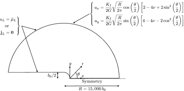
3-1 Schematic of the blunt-crack geometry and boundary conditions used in studying the effects of the chemical potential boundary condition on hydrogen transport near a blunt-crack. . . . . 63 3-2 Hydrostatic stress and equivalent tensile plastic strain ahead of the crack tip after

load in g. . . . . 66 3-3 Lattice hydrogen concentration ahead of the crack tip at different times with the use

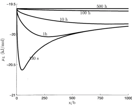
of a constant lattice chemical potential boundary condition. . . . . 67 3-4 Lattice chemical potential ahead of the crack tip at different times with the use of a

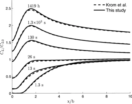
constant lattice chemical potential boundary condition. . . . . 67 3-5 Lattice hydrogen concentration ahead of the crack tip at the end of loading for

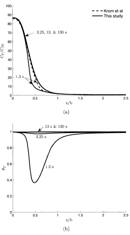
different loading rates with the use of a constant lattice chemical potential boundary condition . . . . 68 3-6 Trapped hydrogen concentration and trapped hydrogen site fraction at the end of

loading for different loading rates with the use of a constant lattice chemical potential boundary condition. . . . . 69 3-7 Lattice hydrogen concentration ahead of the crack tip at the end of loading for

different loading rates with the use of a zero flux boundary condition. . . . . 71 3-8 Lattice chemical potential ahead of the crack tip at different times with the use of a

zero flux boundary condition. . . . . 71 3-9 Trapped hydrogen concentration and trapped hydrogen site fraction at the end of

loading for different loading rates with the use of a zero flux boundary condition. . . 72 4-1 Schematic of the geometry and finite element mesh used for plane-strain tension

sim ulations. . . . . 79 4-2 Contours of total hydrogen concentration prior to mechanical loading for plane-strain

tension sim ulations. . . . . 81 4-3 Contours of total, lattice, and trapped hydrogen concentration at two different

nom-inal end displacements for plane-strain tension simulations. . . . . 82 4-4 Contours of equivalent tensile plastic strain for plane-strain tension simulations of

hydrogen-charged and uncharged specimens. . . . . 83 4-5 Engineering stress versus strain curves for plane-strain tension simulations of

hydrogen-charged and unhydrogen-charged specimens. . . . . 83

4-6 Finite element meshes used for studying mesh sensitivity. . . . . 84 4-7 Contours of equivalent tensile plastic strain for plane-strain tension simulations with

different finite-element meshes. . . . . 85 4-8 Engineering stress versus strain curves for plane-strain tension simulations with

dif-ferent finite-element meshes. . . . . 86 4-9 Schematic and finite-element mesh used in the U-notched three-point bending

sim-u lations. . . . . 90 4-10 Contours of total hydrogen concentration for three-point bending simulations before

load ing. . . . . 90 4-11 Initial variation in the yield strength Y for three-point bending simulations. . . . . . 91 4-12 Contours of equivalent tensile plastic strain for three-point bending simulations of a

hydrogen-charged and an uncharged U-notched metal specimen . . . . . 92 4-13 Contours of equivalent tensile plastic strain near the notch for three-point bending

simulations of a hydrogen-charged and an uncharged U-notched metal specimen. . . 93 4-14 Force versus mid-span deflection curves for three-point bending simulations of a

hydrogen-charged and an uncharged U-notched metal specimen . . . . . 94 4-15 Contours of equivalent tensile plastic strain for three-point bending simulations of a

hydrogen-charged U-Notched metal specimen at different times during loading. . . . 95 4-16 Contours of equivalent tensile plastic strain for three-point bending simulations of a

hydrogen-charged U-notched metal specimen while varying the gradient regulariza-tion param eters. . . . . 96 4-17 Initial yield strength prior to mechanical loading and contours of equivalent tensile

plastic strain for simulations with and without a random variation in the initial yield

strength.... ... ... ... .... ... .. 97

4.1 Initial and boundary conditions for the lattice chemical potential in the plane-strain tension sim ulations. . . . . 77

Representative material properties for a BCC Iron system. . . . . 80 Initial and boundary conditions for the lattice chemical potential in the three-point bending sim ulations. . . . . 88

13 4.2

Introduction

Hydrogen is expected to play an increasingly important role in the development of a "clean" source of energy.1 However, hydrogen is a gas at ambient conditions, and the storage and distribution of hydrogen in its molecular or atomic form is a technological challenge which must be overcome in order to make this source of energy economically viable (cf., e.g., Zittel et al., 2010; Zheng et al., 2011). Atomic hydrogen, being the smallest of gaseous impurities, readily dissolves in and permeates through most materials. Hydrogen dissolution and permeation can be significant at high pressures, and since hydrogen can have deleterious effects on a material it may affect the integrity of structural components used for hydrogen storage and distribution.

Accordingly, it is important to understand and model the coupled diffusion-mechanics response of metallic components used to contain this gas, and this topic is receiving increasing attention because of its potential application to the development of large-scale production, storage, and distribution of hydrogen (cf., e.g., San Marchi et al., 2007; Dadfarnia et al., 2009).

The deleterious effects of hydrogen on the mechanical response of iron and steel are well-known (cf., e.g. Hirth, 1980). The precise microscopic mechanisms by which hydrogen embrittles steels are still not very well understood or modeled. As reviewed by Dadfarnia et al. (2010), research to date has identified two possible mechanisms for hydrogen embrittlement at room temperature: (i) hydrogen-enhanced localized plasticity (HELP), and (ii) hydrogen-induced decohesion (HID). The HELP mechanism is based on the observation that hydrogen reduces the strength of the barriers to dislocation motion and thus enhances the mobility of dislocations. This leads to a reduction in the resistance to plastic flow in regions where the hydrogen concentration is locally high. The precise mechanism by which hydrogen embrittles steels continues to be the focus of intensive theoretical and experimental research (cf., e.g., Ramasubramaniam et al., 2008; Serebrinsky et al., 2004; Novak et al., 2010; Dadfarnia et al., 2010) and is not the focus of this work. Instead, our focus here is on the development of a thermodynamically-consistent continuum-level theory for the diffusion of hydrogen coupled with the thermo-elastic-plastic response of materials. The development of such

'Hydrogen is produced from water by electricity through an electrolyser, and the hydrogen so-produced is a "renewable" fuel only if its produced directly from solar light, or indirectly from a renewable source, e.g., wind- or hydro-power Ziittel et al. (2010).

a theory is an essential prerequisite to any attempt to address the issue of hydrogen-embrittlement related failures in structural components.

It has long been observed that there is an asymmetry between the kinetics of absorption and the kinetics of evolution of hydrogen in steels, in that absorption proceeds with a larger apparent diffusivity than does evolution. This asymmetry in diffusivities is attributed to trapping of the hydrogen atoms at various microstructural "trapping sites," which include interfaces between the matrix and various second-phase particles, grain boundaries, and dislocation cores. A widely-used micro-mechanical model for describing the asymmetry in diffusivities is that of Oriani (1970). His model is based on a crucial assumption regarding the effects of the microstructure on hydrogen transport and trapping. Oriani postulated that within a continuum-level material point, and for a specific range of trap binding energies, the microstructure affects the local distribution of hydrogen in a manner such that the population of hydrogen in trapping sites is always in equilibrium with the population associated with normal interstitial lattice sites.

One of the earliest papers which attempts to couple nonlinear diffusion of hydrogen with large elastoplastic deformation of metals is the seminal paper of Sofronis and McMeeking (1989), who formulated a theory which has Oriani's postulate of "local equilibrium" as one of its central argu-ments. The theory of Sofronis and McMeeking was extended by Krom et al. (1999) to account for the effects of an increase in the number of trapping sites due to plastic deformation, and by Lufrano and Sofronis (1998) to account for lattice-dilatation due to the presence of hydrogen. These compo-nents are all present in the work of Taha and Sofronis (2001) which, with minor modifications, is at present most often used to analyze the effects of interactions of hydrogen transport, elastic-plastic deformation, lattice-dilatation, and hydrogen-induced reduction of the resistance to plastic flow. These coupled theories are not formulated in a thermodynamically-consistent manner and always have Oriani's postulate of "local equilibrium" as a central argument.

The purpose of this work is to develop a thermodynamically-consistent thermo-mechanically-coupled theory accounting for diffusion of hydrogen, trapping of hydrogen, diffusion of heat, and large elastic-plastic deformations within a modern continuum-mechanical framework. In formulat-ing our theory, we limit our considerations to isotropic materials and develop a reasonably general theory in Sections 2.1 through 2.10 of Chapter 2. In Sections 2.11 and 2.12 of Chapter 2 we discuss a special set of constitutive equations which should be useful for applications. We have enhanced our theory with a strain-gradient component in order to avoid mesh-dependent results when modeling materials which plastically soften, this is important to the problem of hydrogen embrittlement of steels since the HELP mechanism suggests that the resistance to plastic flow should decrease in regions of high hydrogen content.

Our specialized theory is similar in spirit to that of Taha and Sofronis (2001), but has the following distinctive characteristics: (i) we do not use Oriani's hypothesis as a central argument to our theory of trapping; rather, based on thermodynamically consistent constitutive choices, we recover his argument as a special case of our theory; (ii) it is phrased entirely at the continuum-level; (iii) it is consistent with modern continuum thermodynamics; (iv) it is properly frame-indifferent; (v) it is not restricted to isothermal conditions.

In Chapters 3 and 4 we present numerical simulations using the chosen constitutive equations and compare our numerical results to some of the published literature. We close in Chapter 5 with a brief summary and listing some outstanding issues that need further research.

In Appendix A we illustrate how our theoretical framework may be used to model hydrogen trapping without the use of Oriani's hypothesis in a thermodynamically-consistent manner. In

Appendix B we provide details on the numerical implementation of our specialized constitutive theory.

Theoretical framework

2.1

Introduction

In this chapter we present our thermodynamically-consistent continuum-level theory for the diffu-sion of hydrogen, trapping of hydrogen, and large elastic-plastic deformation of metals. In Sections 2.2 through 2.10 we present a relatively general theoretical framework. In Sections 2.11 and 2.12 we discuss a special set of constitutive equations which should be useful in applications.

2.2

Notation

We use standard notation of modern continuum mechanics (Gurtin et al., 2010). Specifically: V and Div denote the gradient and divergence with respect to the material point X in the reference configuration; grad and div denote these operators with respect to the point x =

X(X,

t) in the deformed body; a superposed dot denotes the material time-derivative. Throughout, we write Fe-1 = (Fe)-1, Fe-T = (Fe)-T, etc. We write trA, symA, skwA, AO, and sym0A respectively,

for the trace, symmetric, skew, deviatoric, and symmetric-deviatoric parts of a tensor A. Also, the inner product of tensors A and B is denoted by A: B, and the magnitude of A by

IAl

v/A: A.

2.3

Kinematics

2.3.1 Standard kinematics

Consider a macroscopically-homogeneous body B with the region of space it occupies in a fixed reference configuration, and denote by X an arbitrary material point of B. A motion of B is then a smooth one-to-one mapping x = X(X, t), with deformation gradient, velocity, and velocity gradient given by

F = VX, V , L = gradv = ]FF- 1. (2.1)

Following modern developments of large-deformation plasticity theory (cf., e.g., Anand and Gurtin, 2003; Gurtin and Anand, 2005), we assume that the deformation gradient F may be

multiplicatively decomposed as (Kr6ner, 1960; Lee, 1969)

F = FeFP. (2.2)

Here, suppressing the argument t

" FP(X) represents the local deformation of the material in an infinitesimal neighborhood of X due to "plastic" mechanisms. This local deformation carries the material into - and ultimately "pins" the material to - _{a coherent structure that resides in the intermediate space at X (as}

represented by the range FP(X));

" Fe(X) represents the subsequent stretching and rotation of this coherent structure, and thereby represents an "elastic" mechanism.

We refer to FP and F' as the plastic and elastic distortions.

The deformation gradient F(X) maps material vectors to spatial vectors; thus consistent with (2.2), the domain of FP(X) is the reference space, the space of material vectors, and the range of Fe(X) is the observed space, the space of spatial vectors. By (2.2) the output of FP(X) must equal the input of Fe(X); that is

def

the range of FP(X) = the domain of Fe(X) = I(X). (2.3)

We refer to

I(X)

as the intermediate space for X. Thus, for any material point X, FP(X) maps material vectors to vectors in 1(X), and Fe(X) maps vectors in 1(X) to spatial vectors.

By (2.1)3 and (2.2)

L =Le + FeLPFe-l (2.4)

with

Le =

NeFe-1,

and LP =

NPFP-1.

(2.5)

The elastic and plastic stretching and spin tensors are defined through

De = sym L', We = skw Le,

DP = sym LP, WP = skw LP. (2.6)

We assume that

def

J = detF > 0 (2.7)

and hence, using (2.2),

JJeJP where Je d detFe > 0 and J idetFP > 0, f (2.8)

so that F and FP are invertible.

The right polar decomposition of F' is given by

Fe = ReUe, (2.9)

where R' is a rotation, while Ue is a symmetric, positive-definite tensor with

The right elastic Cauchy-Green strain tensor is given by

Ce = (Ue)2 = FeTFe.

Differentiating (2.11) results in the following expression for the time rate of change of Ce 1.

-de = sym(FeTe),

2

a result that we reserve for later use.

We make two basic kinematical assumptions concerning plastic flow:

(i) First, we make the standard assumption that plastic flow is incompressible, so that

JP = detFP = 1 Hence, using (2.8)

and trLP = trDP = 0. J =Je

(ii) Second, from the outset we limit our discussion to isotropic materials, for which it is widely assumed that plastic flow is irrotational in the sense that'

Then, trivially, LP = DP and

Let

p def/3DPI

define an equivalent tensile plastic strain rate.2

tensile plastic strain by

,P(X, t) d

Then, as is traditional, we define an equivalent

I

P(X, ()d(, subject to the initial condition 0

Whenever |DP| z 0,

NP = e |DP|'

defines the plastic

flow

direction, and therefore

with trNP = 0,

DP = T3//2PNP.

'This assumption is based solely on pragmatic grounds: when discussing finite deformations for isotropic materials the theory without plastic spin is far simpler than one with plastic spin.

2

This is a slight abuse in notation in the sense that P is not the material time derivative of -e.

(2.11) (2.12) (2.13) (2.14) (2.15) (2.16) (2.17) O(X, 0) = 0. (2.18) (2.19) (2.20) WP = 0.

#

P = DPFP.

Using (2.1), (2.4), (2.5), (2.16), and (2.20) the rates

j,

#*,

and P are related through

(Vj)F-' =

NeFe-l

+ /3/2PFeNPFe-', (2.21)

a result that we reserve for later use.

2.3.2 An additional microvariable eP

We view e as an isotropic measure of the past history of plastic strain in the material. For the purpose of mathematical regularization and ease of computation in the modeling of materials involving strain softening and localized deformation, following Anand et al. (2012) and Forest (2009), we introduce a positive-valued scalar microvariable eP.

* The microvariable eP serves as an additional microscopic kinematical degree of freedom in developing a gradient theory. Specifically, in contrast to traditional gradient theories which are based on P _{and VP, here we develop a theory which depends on 6, eP, and the gradient}

VeP of the microvariable eP.

2.4

Frame-indifference

A change in frame, at each fixed time t, is a transformation - defined by a rotation Q(t) and a spatial point y(t) - which transforms spatial points x to spatial points

x* = F(x)

=y (t +

Q

(t)(x - o). (2.22)

The function F represents a rigid mapping of the observed space into itself, with o a fixed spatial origin. By (2.22) the transformation law for the motion x =

X(X,

t) has the form

x*(X, t) = y(t) + Q(t)(x(X, t) - o). (2.23) Then, under a change in observer, the deformation gradient transforms according to

F* = QF. (2.24)

The reference configuration and the intermediate structural space are independent of the choice of such changes in frame; thus

FP is invariant under a change in frame, (2.25)

and, by (2.5),

LP and hence DP are invariant under a change in frame. (2.26) Then, (2.2) and (2.24) yield the transformation law

(2.27)

Fe* =

QFe

and

#e* -

QEe+

QFe. (2.28)

Also, by (2.5)1 and (2.28)

Le*

=

QLeQT +

QQ

T (2.29)

and hence

D'* =

QDeQT, and We* = QWeQT +

QQ

T_{. (2.30)}

Further, by (2.9),

Fe* = QReUe (2.31)

and we may conclude from the uniqueness of the polar decomposition that

R'* =

QR',

and Ue is invariant, (2.32)

and on account of the definition (2.11)

Ce is invariant. (2.33)

Finally, the scalar microvariable eP is invariant, and VeP is also invariant since "V" represents a gradient in the reference body.

2.5

Development of the theory based on the principle of virtual

power

Following Anand et al. (2012) and the virtual-power method of Gurtin (2000, 2002) and Gurtin and Anand (2005, 2009) the theory presented here is based on the belief that

o the power expended by each independent "rate-like" kinematical descriport - , 6

eP,

and

Ver - be expressible in terms of an associated force system consistent with its own balance. However, it is not apparent what forms the associated force balances should take. For that reason we determine these balances using the principle of virtual power. We note that the rates

j,#F,

and P are not independent but are constrained through

(V)F-1 -

NeFe-1+

v3/2PFeNPF e-1, (2.34)

which is reiterated from (2.21). Also, VP is simply the material gradient of

eP.

We denote by P an arbitrary part (subregion) of the reference body B with na the outward unit normal on the boundary OP of P. With each evolution of the body we associate macroscopic and microscopic force systems. The macroscopic systems, which are standard, are defined by:

(a) a traction tR(nR) (for each unit vector nR) that expends power over the velocity j on the

boundary of the part;

(b) a body force boa that also expends power over i;3

3

(c) an elastic stress S' that expends power over the elastic distortion rate Fe. The microscopic systems, which are nonstandard, are defined by:

(a) a scalar positive-valued microscopic stress 7r that expends power over the equivalent tensile plastic strain rate P;

(b) a scalar microscopic stress p that expends power over the rate

e&

of the microvariable eP; (c) a vector microscopic stress ( that expends power over the gradient VeP.

(d) a scalar microscopic traction X(nR) (for each unit vector nR) that expends power over

eP

on the boundary of the part;

We characterize the force systems through the manner in which these forces expend power. Given any part P, the power expended on P by material external to P is specified through Wext, and the power expended within P is specified through Wint. Specifically,

Wext (P) = JtR(R) dAR, +IbOR dVR + RP dAR,

JxnnPPAR}(2.35) Wintf(P) = (Se: e + 7rp + p + ( Vep) dVR,

P

where Se, r, p and

(

are defined over the body for all time.

2.5.1 Principle of virtual power

Assume that, at some arbitrarily chosen but fixed time, the fields x, F' (and hence F and FP), and NP are known, and consider the fields

j,

N',

and P as virtual velocities to be specified independently in a manner consistent with (2.34). That is, denoting the virtual fields by

j,

F, and P to differentiate them from fields associated with the actual evolution of the body, we require that

(V)F-' -

NeFe-

+ 3/2PFeNPFe-l. (2.36)

Further, also considering

eP

to be a virtual velocity, and denoting its virtual counterpart by

eP,

we define a generalized virtual velocity to be a list

V = F2 e, jp,

ep),

(2.37)

consistent with (2.36). Writing

Wext(P) = tR(fR) idAR J bOR -dVR R R,

P P P(2.38)

Wint (P) =

J

(Se:

e

+

7tP + Pe + ( -

ve)

dVR,

respectively, for the external and internal expenditures of virtual power, the principle of virtual power is the requirement that the external and internal powers be balanced. That is, given any part P,

Wext (P, V) = Wint (P, V) for all generalized virtual velocities V. (2.39)

2.5.2 Frame-indifference of the internal power and its consequences

We assume that the internal power Wint(P, V) is invariant under a change in frame, and that the virtual fields transform in a manner identical to their nonvirtual counterparts. Then given a change in frame, invariance of the internal power requires that

W*(P, V*) = W(P, V), (2.40)

where V* is the generalized virtual velocity in the new frame. In the new frame S' transforms to Se*,

(

transforms to (*, and from (2.28) P' transforms to

ge*

QFe

+ QFe.

Further,

r, P, p and

eP

are invariant,

since they are scalar fields, and because "V" represents a gradient in the reference body, the

transformation rule for VeP is

(V

eP)*

V

eP.

Thus, under a change in frame Wint(P, V) transforms to

Wi*nt (P, V*)

J

{Se*: (Qe + QFe) + r + peP + .* V } dVR

P _(2.41)

J{QTSe* (Pe+QTQFe) +7 + e +VeP}dV(

P

Then (2.40) implies that

QTSe*.

(Fe

+ QTQFe) + 7P + pep +- VP} dVR

(2.42) = (Se:-+e +rp+ pep + V~') dVR,

P

or equivalently, since the part P is arbitrary,

Also, since the change in frame is arbitrary, if we choose it such that

Q

is an arbitrary time-independent rotation, so that

Q

= 0, we find that

(Se

(QTSe*))

-e +

Since this must hold for all P' and all VeP, we find that the stress Se transforms according to

Se* =

QSe,

(2.43)

and the microforce ( is invariant

(2.44) Next, if we assume that

Q

= 1 at the time in question, so that

Q

is an arbitrary skew tensor, we find that

(SeFeT

):Q =0, or that the stress (S'FIT) is symmetric,

Se Fe T = Fe SeT _(2.45)

Next, to deduce the consequences of the principle of virtual power, assume that (2.39) is satisfied. In applying the virtual balance (2.39) we are at liberty to choose any V consistent with the constraint

(2.36).

2.5.3 Macroscopic force balance

Consider a generalized virtual velocity with both ~P = 0 and (Vj)FP-l - F. For this choice of V, (2.39) and (2.38) yield

6P = 0, so that according to (2.36)

J

tR(fR) dAR+fR aP P bOR dVR J P Se:Pe dVR =

I

(SeFP-T): Vj dVR, P which, by defining may be rewritten as

J

tR(fR) -jdAR aP T_

fSeFp--f

(TR: V P - bORi dVR,

and using the divergence theorem we may conclude that

(tR(nR)- TRIR) dAR R +

J

(Div TR

P

+ boR) -dVR =0.

Since this relation must hold for all P and all

j,

standard variational arguments yield the macro-scopic traction condition

(2.46)

I

(2.47) (2.48) (2.49) - V*)

Ve"

= 0.

(2.50) tR(n1R - RnR,

and the local macroscopic force balance

Div TR

+

bOR = 0, (2.51)

respectively. Furthermore, (2.45) and (2.47) imply that

TRFT = FT T (2.52)

Thus, TR represents the classical Piola stress, and (2.51) and (2.52) represent the local macroscopic force and moment balances in the reference body.

2.5.4 Microscopic force balances

To discuss the microscopic counterparts of macroscopic force balance, consider first a generalized virtual velocity with

j

0 and 6P = 0, and choose the virtual field P arbitrarily. Then, (2.36) yields

fe = - 32PFeNP (2.53)

so that

Se: e = P( 3/2(FeTSe): NP)). (2.54)

Next, define a Mandel stress by

Me de FeTSe (2.55) and define an equivalent tensile stress

a

by the relation

0-

= /2M': NP (2.56)

where in writing the last relation we have used the fact that NP is deviatoric. The power balance (2.39) along with (2.38) yields

0

= Se: -

5

+ -rP) dV (2.57)

P

which using (2.54), (2.55), and (2.56) may be rewritten as

0 =

(

- & P dV (2.58)

P

which must be satisfied for all P and all P. This yields the first microscopic force balance

S7r. (2.59)

Next, consider a generalized virtual velocity with y 0 and P = 0, and choose the virtual The power balance (2.39) along with (2.38) yields the second microscopic field

eP

arbitrarily.

virtual-power relation

I

x(nR) 6P R =

J

(P&P + WP) dVR (2-60)

aP P

to be satisfied for all

eP

and all P. Equivalently, using the divergence theorem,

J

(x(nR) - flR) 6P dA_R +

J

(Dive - p)

eP

dVR - 0, (2.61)

BP P

and a standard argument yields the microscopic traction condition

X(nR) nR, (2-62)

and the second microscopic force balance

Dive - p = 0. (2.63)

2.6

Balance law for the diffusion of hydrogen

Following Anand (2011), let C(X,t) denote the total number of moles of hydrogen atoms per unit reference volume. Hydrogen is absorbed into the metal into normal interstitial lattice sites (NILS), and into trapping sites associated with internal microstructural defects such as dislocation cores, grain boundaries, and interfaces of second-phase particles with the matrix material. Accordingly, we assume that C(X, t) is additively decomposable as

C(X, t) = CL (X, t) + Ca (X, t) (2.64)

where CL(X, t) denotes the number of moles of hydrogen atoms in normal interstitial lattice sites per unit reference volume, Ca (X, t) represents the number of moles of hydrogen atoms in trapping sites per unit reference volume, and a denotes the specific type of trap site in which the hydrogen resides. For brevity we henceforth refer to hydrogen residing in NILS as lattice hydrogen and to hydrogen residing in trapping sites as trapped hydrogen.

For convenience in mathematical modeling of the notion of trapping of a portion of hydrogen content in the material at microstructural trapping sites we consider CL and

Ca

as different species of solutes. Changes in CL and Ca in a part P are then brought about by diffusion of the species across its boundary OP and by the transformation between latticed and trapped hydrogen.

As is standard, the rate of change of lattice and trapped hydrogen in P is given by

OL

= -DivjL - )3 hL-a,

(2.65)

Ca = -Divja + hLa, Va,)

where

jL(X,

t) and

ja

(X, t) are the fluxes of lattice and trapped hydrogen measured as the number of moles of solute atoms per unit area per unit time, and hLa is the transformation rate from

lattice to trapped hydrogen measured as the number of moles of solute atoms per unit volume per unit time. At this point in the development of the theory it is convenient to allow for non-zero fluxes

ja

for the trapped hydrogen; later, we shall make specific assumptions which will result in

ja = 0.

2.7

Balance of energy. Entropy imbalance. Free-energy imbalance

Our discussion of thermodynamics follows Gurtin et al. (2010, Section 64), and involves the following fields

ER the internal energy density per unit reference volume,

77R the entropy density per unit reference volume,

qR the heat flux per unit reference area,

qR the external heat supply per unit reference volume, 9 > 0 the absolute temperature,

pL the chemical potential for the lattice hydrogen,

ya the chemical potential for the a-th trapped hydrogen species. The balance law for energy, is

EJRdVR

JqR 'n dAR JqR dVR +)/Vext (P)JLiL -nR

dAR

-S JaanR dAR, (2-66)

P OP P aP a

g

where the last two terms in (2.66) represents the energy contribution into P by the lattice and trapped hydrogen (Gurtin, 1996). Since Wext(P) = Wint(P), using (2.35)2, and applying the divergence theorem, we obtain

I 8

R dVR

J

(Se: - e - wr + pNP ±. - Ver - Div q + qR

PP (2.67)

- PLDivjL - jL VPL +Y - paDivja -

ja

Vpa dVR.

Use of the balance laws (2.65) and the fact that (2.67) must hold for all parts P, gives the local form of the energy balance as

9R = Se: Fe

+

7 - Pe + -Ve - DivgR + qR

+ pLCL - L V/IL + (Paoa - a ' V/a + (PL - /ia)hL-*a (2.68) Note that while the "elastic power" Se:

N

itself is invariant, neither the stress Se nor the elastic distortion rate F' are invariant under a change in frame. Accordingly, as is standard, we express this elastic power in terms of Ce and a power-conjugate stress measure. Let

then, since SeFeT = FeTCFeT, (2.45) yields

Te T. (2.70)

Thus Se: e - Te:FeT

Pe, and in view of (2.12), 1

Se:e Te:de (2.71)

2

Finally, using this result the local energy energy balance (2.68) may be rewritten as 1

R = -Te: Ce + 7rp + pp

+

.V - DivqR + qR

2 _(2.72)

+ 2LUL - L V VL +

S

a a - ja ' V/a (PL - pa)hL -(27

The second law takes the form of an entropy imbalance

TRdR -

J

R RnR dAR + R (2.73)

P BP P

and the local entropy imbalance has the form of

/R > -Div q

+

(2.74)

Let

aRf ER OIR (2.75)

denote the (Hemholtz) free energy per unit volume of the reference body. Then use of (2.72), (2.74) and (2.75) yields the local free-energy imbalance

1 .1

~~PR

~

- T: I -]R _{i-P - p~P} -.Ve~ -+-OR + IR79 -' -qR' 2 (2.76) - MLCL +jL - VjL + -3 a a

+/

a ' a - (AL - /Ia)hL-+a 0.

We use this inequality as a guide in developing a suitable constitutive theory.

For later use we define the dissipation density D > 0 per unit volume per unit time by

1 1

D = -Te~a + x# F- .S qR - So

2 _0(2.77)

+ pLCL - L V VL

+

(/aeoa - ja ' e ±a (/IL - pa)hL-o) -R - 7R >

0-In the preceding discussion we have introduced four stress measures: S', TR, M', and Te. Before closing this section we note that since the Piola stress TR is related to the symmetric

Cauchy stress T in the deformed body by the standard relation

the definitions (2.47), (2.69), and (2.55) yield

Se, Te, Me, and the Cauchy stress T:

Se = JTFe -T e" = JFe-1 TF e-T

the following relations between the stress-measures

and Me = JFeTTFe-T = CeTe. (2.79)

2.8

Constitutive theory

2.8.1 Basic constitutive equations

Guided by the free-energy imbalance (2.76), we first consider the following constitutive equations for the free energy OR, the stress T', the entropy 77R, the chemical potentials pL and p, the scalar

microscopic stress ir, the scalar microscopic stress p, and the vector microscopic stress

(:

Te -

te(A),

7R =R(A), pL = AL(A), pa = a(A), 7 = -fr(A), (2.80)

where A denotes the list

A = (Ce IP, eP, VeP,19, CL,

Ca).

(2.81)

Further, we assume that the scalar and vector microscopic stresses -r, p, and ( can be decom-posed into energetic and dissipative parts

7 = 7Ten + 7rdis,

P = Pen + Pdis, =

den

+ dis

2.8.2

Thermodynamic restrictions

Using (2.80)1 the local free-energy imbalance (2.76) may be rewritten as

(

&'R(A) _e

ace

2 )

+(a R(A) ( OV eP

'+ ( R(A)

Oa +jL -VOLp +

_ji

_Vpac - (AL

cc

- a)hLna + QR ' V7 <K

0-We identify the energetic components of 7r, p and

(

as

def O'V)R(A) WFen

IlE

def V)R (A) Pen = eP (2.84) def 8V'a(A) sen l _fee it

such that using (2.82) and (2.84) in (2.83) the local free-energy imbalance may be written as

O

R(

+ y7R ) +

DbR (A)

ac,

aPR (A)

(ce

1Te

_{:a~ (DCLf}

- Aa )a -- 7disp - Pdise" - dis . P

-

AL

)

OL

(2.85)

+jL -VyL +I (ja VPa - (PL - Ial)hLaa)

+

I R V < 0.

79

This inequality must hold for all values of A. Since e,

de,

OL,

and

Oa

appear linearly, their "coefficients" must vanish, for otherwise 0, Ce, CL, and Ca may be chosen to violate (2.85). We are therefore led to the thermodynamic restriction that the free energy determines the stress T',

+ 77R ) +

(OeR(A)

(9

eP

-

P,)

O R(A) aCa -ta) -PL) CL (2.83) R a,,A

- V

' +

_CL

the entropy IR, and the chemical potentials PL and Mt, through the "state relations" T' 2 OOR(A) ace O~bR(A) 7 9 _{() ' >} (2.86) M aCL

(90R

Ac

and the dissipation density (2.77) reduces to

D = 7Tdis( -f-

Odis-iIi('V

- - a' ea L-jL1hVPL L- a) - V > 0. (2.8 7)

2.8.3 Dissipative constitutive equations

Next, guided by the dissipation inequality (2.87), and experience with existing plasticity theories, we make the following constitutive assumptions:

(1) As is classical in finite deformation theories of isotropic plasticity (cf., Gurtin et al., 2010), we assume that the direction of the plastic flow coincides with the direction of the deviatoric Mandel stress, that is DP is codirectional with M8. The plastic flow direction (2.19) is then given by

DP me

NP = = 0 _(2.88)

|DP| |Me |

Thus, the equivalent tensile stress 6 = V3//2 Me: NP, defined in (2.56), is given by

v/

= 3/2Me |. (2.89)

Using (2.20), (2.88), and (2.89) the plastic stretching DP may be written as

DP = 3 . (2.90)

2

(2) A constitutive equation for 7tdis of the form

7dis = dis(A) with A = (EPeP, , CL, Ca), (2.91)

which for simplicity is independent of P and

eP.

Here

Ydis > 0, (2.92)

a positive-valued scalar with dimensions of stress, represents the classical flow resistance of the material. The initial value at a reference temperature do and at reference concentrations

C and C., C

YO

Zre

dis(0,1 0, ino , Cste Cth) > 0,

represents the inial yield strength. Let

f(A) def fdis(A) + Yen(A) with Yen

_gren

represent the combined dissipative and energetic parts of the constitutive equation for r. Then the microscopic force balance (2.59) requires that

u = Y when P>0. _(2.95)

(3) Based on (2.95) we introduce a yield function def

f

=&- Y(A) 0, (2.96)

which limits the admissible deviatoric stresses MI. Then, as is standard, a rate-independent theory is based on the Kuhn-Tucker conditions

0P>,

f

0, and Pf-=0, (2.97)

together with the consistency condition

when f = 0. _(2.98)

(4) We assume further that the dissipative microscopic stresses Pdis and (dis are given by consti-tutive equations

Pdis =

$dis

(E, P, Jp

2

P

,

Gep, V

", V, CL), Ca),

(2.99)

5) We assume that the transformation rates hLaa depend on the equivalent tensile plastic strain

2P,

the temperature d, and the concentrations CL and Ca

hL-+a= hL-+(E,'0,dCL,Ca), Va. (2.100)

More generally, as discussed in Appendix A, the transformation rates hL a may depend on the conjugate driving force (PL - A,); cf. eq. (2.87).

(2.93)

(2.94)

To the constitutive equations above we append a Fourier-type relation for the heat flux, and Fick-type relations for the flux of the diffusing hydrogen,4

qR=

jL = ~ML(A )VPL, (2.101)

ja

= -a( A)V/a,

J

where K is a thermal conductivity tensor, ML and Ma are mobility tensors, and A denotes the list

A

= (C e, CP, 79, CL, Ca). (2.102) Finally, the dissipation density (2.87) may be written as

1

D=7disP + Pdisep + (dis- VP + -VIW KVO

+ V/pL M LV/L + ( a- MaVa ± (,L - Ua)hLa) > 0. (2.103) We also assume that the terms in (2.103) individually satisfy

?disP > 0 for P > 0, (2.104) Pdis e > 0 for

eP

> 0, (2.105) dis-Vep > 0 for VP# O, (2.106) and VO - KV9 > 0, (2.107) VpL MLV/IL > 0, (2.108)

(AL - pa)hL-*a > 0, Va, (2.109)

Vya- MaV/a > 0, V a. (2.110)

Thus, note that the thermal conductivity tensor K and the mobility tensors ML and Ma are positive-semidefinite.

2.8.4 Further consequences of thermodynamics

In view of (2.80)1, (2.84), and (2.86) we have the first Gibbs relation, -1

R -+ 7en + Pen + en - LOL + t-(2.111)aa

4

which, with (2.75), yields the second Gibbs relation 1

iR = R + I Te: & + 7enP + Pene + en *V + ILOL +

P-jaa-2 (2.112)

Using the balance of energy (2.72), the second Gibbs relation (2.112), the decomposition of the scalar and vector microscopic stresses (2.82), and equations (2.101), we arrive at the entropy balance

'o7R = -DivqR qR + TdisP + Pdise + dis

+

VPL - MLVL (Vp-. a MaVPa

+

(ML - a)hL ₄

a)-Granted the thermodynamically-restricted constitutive relations (2.84) and (2.86), along with the decomposition (2.82), this balance is equivalent to the balance of energy.

Next, from (2.75), the internal energy density is given by

SR(A)

<R(A) + 7 R (A) (2.114)

and, as is standard, the specific heat is defined by

def O R(A)

C = 7 (2.115)

Hence, from (2.114)

c = (A)

and use of (2.86) gives

Next, using (2.80)3 and (2.117)

- a 2 _(A) 8d 2

(A)

- 80C L

+ iR(A) + 79 4W ) (2.116) (2.117) a2cR(A) C= -7) _a?2 a2 _{(A) P}

-z

eP

82

(A) -W&e

-z

a

- _-99VeP~c

89

a2

(A)

e

-I- C

808ag Ca,

(2.118) (2.113)

which using (2.84) and (2.86) yields

oIR &o :a en. e O P p

Then, using (2.119) in (2.113) gives the following partial differential equation for the temperature

c5=-Divqa+qa+disP+Pdis+dis' +1 -- e

aT

+d ""7ren dPen

2 09 (9

+ O "en - V + 9

OL

+ VAL - MLVPL (2.120)

+

(

COa + Vy . MatVa + (PL -

pa)hLa).-2.9

Isotropy

The following definitions help to make precise our notion of an isotropic material (cf., Anand and Gurtin, 2003):

(i) Orth+= the group of all rotations (the proper orthogonal group);

(ii) the symmetry group ga, is the group of all rotations of the reference configuration that leaves the response of the material unaltered;

(iii) the symmetry group g, at each time t, is the group of all rotations of the intermediate space

that leaves the response of the material unaltered.

We now discuss the manner in which the basic fields transform under such transformations, granted the physically natural requirement of invariance of the stress-power (2.71), or equivalently, the requirement that

Se:

e

and Te:

de

be invariant. (2.121)

2.9.1 Isotropy of the reference configuration

Let

Q

be a time-independent rotation of the reference configuration. Then F -* FQ, and hence FP -* FPQ, F' is invariant, and hence C' is invariant,

so that

Pe and

de

are invariant. We may therefor use (2.121) to conclude that

Se and Te are invariant. Thus

* The constitutive equations (2.80) are unaffected by such rotations of the reference configura-tion.

Turning our attention next to the constitutive equation (2.101)1 for the heat flux, a standard result from the theory of finite thermoelasticity is that under a symmetry transformation

Q

of the

(2.122)

(2.123)

reference configuration, the temperature gradient V9 and the heat flux qR transform as (cf., Gurtin et al., 2010, Section 57.8)

V?9

_{-+ Q}

T

_V',

qR- -R Q q.

Hence, from (2.101)1 the thermal conductivity tensor K must obey

for all rotations

Q

E 9

R-(2.125)

(2.126) By an analogous argument, the mobility tensors ML and Ma must obey

ML (A) = QT

ML ()Q

and

nc(A)

= QT

na(A)Q

for all rotations

Q

E

gR-We refer to the material as initially isotropic (and to the reference configuration as undistorted) if

9R = Orth+ (2.128)

so that the response of the material is invariant under arbitrary rotations of the reference space. Henceforth we restrict attention to materials that are initially isotropic.

In this case, the thermal conductivity and the mobility tensors have the representation

K(A)

= k

(A)1,

with r, > 0 a scalar thermal conductivity, and

ML rnL(A)1 _{and Ma(A) =fia,(A)1,}

with mL > 0 and ma > 0 scalar mobilities.

2.9.2 Isotropy of the intermediate structural space

Next, let

Q,

a time-independent rotation of the intermediate space, be a symmetry transformation. Then F is unaltered by such a rotation, and hence

Fe -+ Fe Q and FP -+ QT FP,

and also

Ce -+ QTCeQ,

de

-_ QT

aQ,

then (2.132) and (2.121) yield the transformation laws

Se

-+ Q

T

SeQ,

Te - Q

T

TeQ.

K(A) = QTk(A)Q (2.127) (2.129) (2.130) Fe - QTFeQ (2.131) (2.132) (2.133)

Thus, with reference to the constitutive equations (2.80) together with (2.129) and (2.130) we conclude that

'VR(A) = OQ AQ),

Q

T

ie(A)Q

=

Te(Q

T

AQ),

AL(A)

= AL (QTAQ),

Aae(A)

= JA(Q T_AQ),

-(A)

= f(QTAQ),

(2.134)

b(A) = b(QT

_AQ),

(A)

=

(Q

T

_AQ),

k(A) = k(QTAQ), rnL(A) = fnL(Q Q) fn(X=

rfna(Q

T

_AQ),

with

QTAQ = (QTCeQ,0, e, QTVepd, CL, Ca), (2.135)

Q

T

XQ = (Q

T

CeQ, p,, CL, Ca),

which must hold for all rotations

Q

in the symmetry group 9, at each time t.

We refer to the material as one which is continually isotropic, if in addition to the referential isotropy discussed in the previous subsection,

91 = Orth+ (2.136)

so that the response of the material is also invariant under arbitrary rotations of the intermediate space at each time t. Henceforth we restrict attention to materials that are not only initially, but also continually, isotropic.

In this case, the response functions OR, T', rR, AL,

Aa,

ft , k, frL, and rh must also each

be isotropic.

2.9.3 Isotropic free energy

An immediate consequence of the isotropy of the free energy is that the free energy function has the representation

PR(C, e e, Vep, 0, CL, CC) ='R(IC, P, eP, I 0, CL, Ca) (2.137)

where

is the list of principal invariants of Ce. Thus, from (2.86)1, it follows that

T' = 2 _Te~2 e _ace,

IVeP1,

CLI Ca) (2.139)

and that T' is an isotropic function of Ce. Then since the Mandel stress can be expressed by (cf.

(2.79))

Me = CeTe (2.140)

we find that Te and Ce commute,

CeTe TeCe (2.141)

and hence the Mandel stress Me is symmetric.

Next the spectral representation of Ce is

3

Ce e2(A)2ri

o

ri (2.142)

where (ri, r', r') are the orthonormal eigenvectors of Ce and Ue, and (A', A', Ae) are the eigenvalues of Ue. Instead of using the invariants Ice, the free energy

@R

for isotropic materials may be alternatively expressed in terms of the principal stretches as

Then, by the chain-rule and (2.86)1, the stress T' is given by

ace

3

OO2

S&R(A',

Ae,A', 0,

eP,

IV

eP ,,CL,

C,)

aMx

1

e

ace

3i OOR (Ae, Ae

~,e

__

~')

a

~.

2e(2.144)

Assume that the squared principal stretches (M )2 are distinct, so that the (M )2 and the principal directions r may be considered as functions of Ce; then

9 _(2.145)

ace

and, granted this, (2.145) and (2.144) imply that

i=1 aOR(AeAe, _AePePV

Next, since Me = Cere, use of (2.142) and (2.146) gives the Mandel stress as

Me =3e O)R (A e A~ e , eP, ep, IV ,),%C, t9 C,,)

(2.147) i=1

Let

3

e dew _vales

denote the logarithmic elastic strain with principal values

(2.148)

(2.149)

and consider a free energy of the form

'OR(A , Ae, Ae, 0, ep,

IVLeP1,,d,

CL, Cc,) OR (Ee, Ee, Ee, EP, eP, |V eP 1, CL, Ca) (2.150)

so that, using (2.147),

e R(Ee, Ee, Ege, 0, eP, |VeP 1, V, CL, Ca) e

m =E1 r e re (2.151)

With the logarithmic elastic strain defined by (2.148), and bearing (2.150) and (2.151), for isotropic

elastic materials we henceforth consider a free energy of the form

OR ='(IEe, 0, eP,

IV eP,

0, CL, Ca) (2.152)

with 14e a list of principal invariants of E', or equivalently a list of principal values of E'. The Mandel stress is finally given by

me - OOR (lEe, 0, eP,

IVeP

10, CL, Ca) (2.153)

BEe Further, using (2.146) in (2.79),

T = J- 1Fe TeFeT

_ J-1ReUeTeUeReT

ja R 1

~e(Ae,

Ae, A , c'P, eP, IV eP 79 ,CL, Cc,)

- J-R e e 1 3 20 r) ReT (2.154)

and using (2.147) the Cauchy stress is given by

T = J-ReMeReT (2.155)

re (9 re