www.atmos-chem-phys.net/16/15689/2016/ doi:10.5194/acp-16-15689-2016
© Author(s) 2016. CC Attribution 3.0 License.
Airborne observations of far-infrared upwelling radiance
in the Arctic
Quentin Libois1, Liviu Ivanescu1,2, Jean-Pierre Blanchet1, Hannes Schulz3, Heiko Bozem4, W. Richard Leaitch5, Julia Burkart6, Jonathan P. D. Abbatt6, Andreas B. Herber3, Amir A. Aliabadi7, and Éric Girard1
1Department of Earth and Atmospheric Sciences, Université du Québec à Montréal, Montréal, Canada
2Centre d’applications et de recherches en télédétection (CARTEL), Université de Sherbrooke, Sherbrooke, Canada 3Alfred Wegener Institute, Helmholtz Center for Polar and Marine Research, Bremerhaven, Germany
4Johannes Gutenberg University of Mainz, Institute for Atmospheric Physics, Mainz, Germany 5Environment and Climate Change Canada, Toronto, Canada
6Department of Chemistry, University of Toronto, Toronto, Canada
7Atmospheric Innovations Research (AIR) Laboratory, School of Engineering, University of Guelph, Guelph, Canada
Correspondence to:Quentin Libois ([email protected])
Received: 10 August 2016 – Published in Atmos. Chem. Phys. Discuss.: 26 September 2016 Revised: 29 November 2016 – Accepted: 2 December 2016 – Published: 20 December 2016
Abstract. The first airborne measurements of the Far-InfraRed Radiometer (FIRR) were performed in April 2015 during the panarctic NETCARE campaign. Vertical profiles of spectral upwelling radiance in the range 8–50 µm were measured in clear and cloudy conditions from the surface up to 6 km. The clear sky profiles highlight the strong depen-dence of radiative fluxes to the temperature inversion typical of the Arctic. Measurements acquired for total column wa-ter vapour from 1.5 to 10.5 mm also underline the sensitiv-ity of the far-infrared greenhouse effect to specific humidsensitiv-ity. The cloudy cases show that optically thin ice clouds increase the cooling rate of the atmosphere, making them important pieces of the Arctic energy balance. One such cloud exhib-ited a very complex spatial structure, characterized by large horizontal heterogeneities at the kilometre scale. This em-phasizes the difficulty of obtaining representative cloud ob-servations with airborne measurements but also points out how challenging it is to model polar clouds radiative ef-fects. These radiance measurements were successfully com-pared to simulations, suggesting that state-of-the-art radiative transfer models are suited to study the cold and dry Arctic atmosphere. Although FIRR in situ performances compare well to its laboratory performances, complementary simu-lations show that upgrading the FIRR radiometric resolu-tion would greatly increase its sensitivity to atmospheric and cloud properties. Improved instrument temperature stability
in flight and expected technological progress should help meet this objective. The campaign overall highlights the po-tential for airborne far-infrared radiometry and constitutes a relevant reference for future similar studies dedicated to the Arctic and for the development of spaceborne instruments.
1 Introduction
Since the early days of weather satellites, remote sensing in the infrared (IR) has been used to study the vertical structure of the Earth atmosphere (e.g. Conrath et al., 1970). Most in-struments currently deployed, such as the Moderate Resolu-tion Imaging Spectroradiometer (MODIS; King et al., 2003), the Atmospheric Infrared Sounder (AIRS; Aumann et al., 2003) and the Infrared Atmospheric Sounding Interferometer (IASI; Blumstein et al., 2004), do not measure atmospheric radiation beyond approximately 15 µm, though, because sensing far-infrared radiation (FIR; 15 µm < λ < 100 µm) generally requires a different technology (Mlynczak et al., 2006). However, probing the atmosphere in the FIR could provide valuable information and complement current obser-vations. The FIR range includes the strongly absorbing pure rotation band of water vapour and coincides with a maxi-mum in the water vapour continuum strength (Shine et al., 2012). As such, it is especially promising for remote sensing
of water vapour in the coldest regions of the atmosphere, that is the upper troposphere and the stratosphere (Rizzi et al., 2002; Shahabadi and Huang, 2014), and the polar regions in general (Turner and Mlawer, 2010; Blanchet et al., 2011; Palchetti et al., 2015). The emission maximum of Planck’s function shifts towards the FIR with decreasing temperature, so that increasingly more energy is emitted from this spec-tral region (Merrelli and Turner, 2012) compared to the more widely used 6.7 µm vibrational-rotational band (Susskind et al., 2003). Hence in cold atmospheres more than half of the radiation is lost to space from the FIR domain (Clough et al., 1992). The FIR signature of clouds also carries much information about cloud phase, optical thickness, particle ef-fective size and particle shape for ice clouds (Rathke, 2002; Yang et al., 2003; Baran, 2007). This assessed sensitivity has recently stimulated the development of retrieval algo-rithms for ice cloud properties (e.g. Blanchard et al., 2009; Palchetti et al., 2016). Observing long-term changes in the FIR emission of Earth could eventually provide valuable in-sight into the physical processes underlying climate change (Huang et al., 2010).
As a consequence, in the last 3 decades a number of scien-tific teams have demonstrated the need for improved obser-vation of the Earth in the FIR (e.g. Mlynczak et al., 2002; Harries et al., 2008). In the meantime, several FIR spec-trometers were developed. The Atmospheric Emitted Ra-diance Interferometer (AERI; Knuteson et al., 2004) has been extensively used for atmospheric profiling and cloud remote sensing (Turner and Löhnert, 2014; Cox et al., 2014). The Far-InfraRed Spectroscopy of the Troposphere (FIRST; Mlynczak et al., 2006) and the Radiation Explorer in the Far-InfraRed – Prototype for Applications and Development (REFIR-PAD; Palchetti et al., 2006) were developed within the framework of the satellite projects Climate Absolute Ra-diance and Refractivity Observatory (CLARREO; Wielicki et al., 2013) and REFIR (Palchetti et al., 1999), respectively. These instruments primarily aim at better constraining the radiative budget of the atmosphere and have been operated from gondola and from the ground (Bianchini et al., 2011; Mlynczak et al., 2016). The Tropospheric Airborne Fourier Transform Spectrometer (TAFTS; Canas et al., 1997) has been used to explore the radiative properties of water vapour (Green et al., 2012; Fox et al., 2015) and to investigate the radiative properties of cirrus clouds (Cox et al., 2010). So far, all these spectrometers have been extensively used to im-prove the parameterization of the water vapour absorption lines and continuum in the FIR (Delamere et al., 2010; Li-uzzi et al., 2014), in order to refine radiative transfer codes (Mlawer et al., 2012) and climate simulations (Turner et al., 2012).
Further understanding the radiative properties of the at-mosphere in the FIR is of uttermost in the Arctic because proportionately more energy is emitted from cold regions at FIR wavelengths while at the same time lower water vapour column increases atmospheric transmittance (Clough et al.,
1992). Although FIR spectrometers have been used from the ground in Alaska and Northern Canada (Mariani et al., 2012; Fox et al., 2015), we are not aware of any such air-borne measurements in the Arctic. The panarctic NETCARE (Network on Climate and Aerosols: Addressing Key Un-certainties in Remote Canadian Environments, http://www. netcare-project.ca) aircraft campaign, which took place in April 2015, attempted to fill this gap. This 4-week cam-paign investigated the radiative properties of the atmosphere in clear and cloudy conditions, with a stress on aerosols. These scientific flights offered the possibility to probe the atmosphere in situ, thus providing a valuable complement to the extensive ground observations performed at well instru-mented sites such as Summit (e.g. ICECAPS project; Shupe et al., 2013) and Eureka (e.g. CANDAC network; Mariani et al., 2012). Altogether, these initiatives aim at refining our understanding of the radiative budget of the Arctic and the critical role clouds play in it, in the continuity of the seminal Surface Heat Budget of the Arctic Ocean (SHEBA) program (e.g. Shupe et al., 2006).
While most reported airborne FIR observations consist of constant altitude flights, vertical profiles of spectral radiance are very instructive to understand the vertical structure of the energy budget of the atmosphere (Mlynczak et al., 2011). For this reason, most measurements taken with the Far-InfraRed Radiometer (FIRR; Libois et al., 2016) during the campaign consisted of vertical profiles of upwelling radiance from the surface up to about 6 km. The FIRR was developed as a tech-nology demonstrator for the Thin Ice Clouds in Far-InfraRed Experiment (TICFIRE; Blanchet et al., 2011) satellite mis-sion, the primary focus of which is on the water cycle in the Arctic, and ice clouds in particular. Like cirrus at mid-latitudes (Cox et al., 2010; Maestri et al., 2014), ice clouds encountered in the Arctic significantly affect the atmosphere radiative budget in the FIR, especially because they can fill the whole troposphere (Grenier et al., 2009). In very dry con-ditions, they act as particularly efficient emitters that radia-tively cool the atmosphere (Blanchet et al., 2011). Unlike the tropics, such ice cloud layers occur at any altitude, from the ground to the stratosphere (polar stratospheric clouds). Their radiative effect depends on their physical properties (Maestri, 2003; Maestri et al., 2005) but is also very dependent on moisture (Cox et al., 2015), making the interactions between water vapour and Arctic clouds particularly complex.
In the context of TICFIRE, there were four main reasons of flying the FIRR in the Arctic: (1) assessing the FIRR radio-metric performances in airborne conditions meant to mimic as closely as possible satellite nadir observations; (2) vali-dating radiative transfer simulations in the FIR for clear and cloudy Arctic conditions through radiative closure experi-ments; (3) verifying the spectral signature of clouds radiance in situ; (4) investigating the sensitivity of FIRR measure-ments to atmospheric characteristics and better understand-ing the radiative budget of the Arctic atmosphere. The FIRR measurements taken during the campaign are presented in
Sect. 2, along with complementary observations relevant to the radiative properties of the Arctic atmosphere. Five case studies are then detailed in Sect. 3 and serve as a basis to as-sess FIRR performances in airborne conditions and explore its sensitivity to atmospheric conditions. The sensitivity to temperature, humidity and cloud properties is further inves-tigated in Sect. 4 using radiative transfer simulations. Based on this unique experience, recommendations are provided for future operations of instruments similar to the FIRR in such airborne campaigns.
2 Materials and methods 2.1 The NETCARE campaign
The panarctic PAMARCMIP/NETCARE campaign (here-inafter NETCARE campaign) comprises many collaborators including the following institutions: Alfred Wegener Insti-tute (AWI), University of Toronto, Environment and Climate Change Canada (ECCC) and more parties listed under the website. The campaign, which involved the two instrumented Basler BT-67 Polar 5 and Polar 6 aircraft (e.g. Ehrlich and Wendisch, 2015), started in Longyearbyen (Spitzbergen) on 5 April with 1-week delay due to harsh weather condi-tions. There, only one flight dedicated to calibration was per-formed. Then the aircraft flew across Station North (Green-land) and operated around Alert, Nunavut (Canada), from 7 to 9 April. Afterwards, they moved to Eureka, Nunavut (Canada), and stayed there until 17 April. They continued to Inuvik, Northwest Territories (Canada), where Polar 6 op-erated until 21 April, while Polar 5 headed towards Barrow (Alaska). No flights were performed with Polar 6 from 14 to 19 April due to cloudy conditions at Eureka and techni-cal problems with the aircraft. The two aircraft had different scientific objectives, with Polar 5 mostly dedicated to sea ice studies and Polar 6 to aerosol and cloud studies. In the fol-lowing, only Polar 6 operations are detailed, which consist of 10 scientific flights, amounting to 50 h of campaign flight time.
The NETCARE campaign aimed at better understanding aerosol transport into the Arctic in the early spring and its influence on ice cloud formation. One of the objectives was to characterize at the same time the microphysical and ra-diative properties of ice clouds, along with the nature of the aerosols, in order to further explore the conditions in which optically thin ice clouds form and how their microphysics depend on background aerosols. Many instruments were in-stalled aboard Polar 6, including basic meteorology and ra-diation sensors, cloud microphysics instrumentation, particle counters, trace gas monitors and instruments for monitoring aerosol composition (e.g. Leaitch et al., 2016). Each flight was planned based on forecasts of clouds and transported pollution as well as the location of the A-Train satellite con-stellation (Stephens et al., 2002). The atmosphere was
gen-erally probed vertically from the surface (∼ 50 m) to approx-imately 6000 m (or the other way round) in about 50 min. To this end, the aircraft followed quasi-spirals of diameter 10 km.
2.2 In situ observations
2.2.1 The Far-InfraRed Radiometer
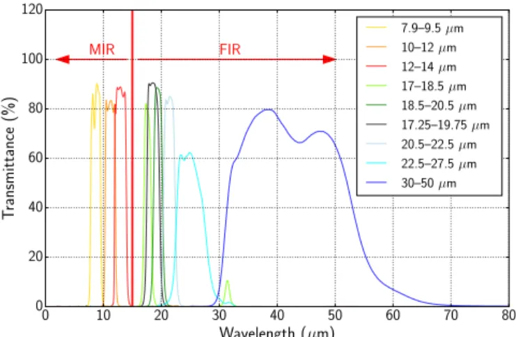
The FIRR (Libois et al., 2016) uses a filter wheel to measure atmospheric radiation in nine spectral bands ranging from 8 to 50 µm (Fig. 1). In this sense it is very similar to the Mars Climate Sounder (McCleese et al., 2007) and the Diviner Lu-nar Radiometer Experiment (Paige et al., 2010), which use uncooled thermal sensors to probe radiation in the FIR. The FIRR sensor is a 2-D array of uncooled microbolometers coated with gold black (Ngo Phong et al., 2015), and radio-metric calibration is achieved with two reference blackbodies (BB) at distinct temperatures. The latter consist of cavities whose temperature and emissivity are well known, so that the radiance they emit is accurately estimated. During the NETCARE campaign, the FIRR was onboard Polar 6 and measured upwelling radiance directly through a 56 cm long vertical chimney. At the bottom of the chimney, a rolling door (Fig. 2) opened during the flight but remained closed other-wise to prevent dust or blowing snow from entering the in-strument. Although the FIRR has a nominal field of view of 6◦corresponding to a 20 pixels diameter area on the sensor, here only a 15 pixel diameter area is used to avoid the small vignetting on the edges of the illuminated area. This corre-sponds to a field of view of 4.5◦, which translates into a foot-print of 7.8 m at a 100 m distance and 470 m at 6000 m. Since the temperature aboard the unpressurized cabin quickly var-ied between approximately 0 and 15◦C, the ambient black-body (ABB) was maintained at 15◦C, while the hot black-body (HBB) was set to 45 or 50◦C. These correspond to BB nominal temperatures in flight but some experiments were performed with different BB temperatures depending on the environmental constraints, which is not problematic since the instrument’s response is linear in this range of temper-ature (Libois et al., 2016). One FIRR measurement sequence lasts 210 s, during which approximately 40 s are used to ac-tually take measurements and 170 s are spent rotating the filter wheel and the scene selection mirror. A sequence con-sists of two calibration sequences (one on the ABB and one on the HBB) followed by three scene sequences, each se-quence corresponding to one complete rotation of the filter wheel that measures all nine filters in approximately 40 s. For each spectral band, 100 frames are acquired at 120 Hz and then averaged to provide a single 2-D image. One spec-tral measurement thus corresponds to a 0.8 s long acquisition and no supplementary temporal average is performed, high-lighting the potential for fast scanning compared to interfer-ometers that usually require averaging over several spectra to achieve comparably high performances (e.g. Mlynczak et al.,
0 10 20 30 40 50 60 70 80 Wavelength (µm) 0 20 40 60 80 100 120 T ransmittance (%) FIR MIR 7.9–9.5 µm 10–12 µm 12–14 µm 17–18.5 µm 18.5–20.5 µm 17.25–19.75 µm 20.5–22.5 µm 22.5–27.5 µm 30–50 µm
Figure 1. Spectral transmittances of the nine filters of the FIRR, whose band pass are indicated in the legend. Three filters cover the mid-infrared (MIR) and six are in the far-infrared (FIR).
2006). Such acquisition rate is essential when looking at het-erogeneous or quickly moving targets, as is the case from an aircraft or satellite view. It is the main advantage of trading spectral resolution for higher signal levels. Note, though, that measurements in successive spectral bands are offset tempo-rally, hence spatially, which has to be borne in mind at the stage of data interpretation. In this study, the FIRR is not used as an imager, and thus the data presented here corre-spond to averages over the selected area of 193 pixels. In this configuration, the radiometric resolution of the FIRR in labo-ratory conditions is essentially limited by detector noise and is about 0.015 W m−2sr−1. This corresponds to noise equiv-alent temperature differences of 0.1–0.35 K for the range of temperatures investigated in this study. The radiometric res-olution is nearly constant for the seven bands ranging from 7.9 to 22.5 µm because the absorptivity of the gold black coating is spectrally uniform and the filters all have simi-lar maximum transmittances. It is approximately 30 % less for the filters 22.5–27.5 µm and 30–50 µm because of limited filter transmittance for the band 22.5–27.5 µm and reduced package window transmittance for the band 30–50 µm. Such performances compare well with similar airborne spectrora-diometers (e.g. Emery et al., 2014) and satellite sensors (e.g. MODIS).
A critical issue during the campaign was the tempera-ture stability of the instrument in operation. Indeed, the first flights were characterized by excessively noisy measure-ments, especially in the 30–50 µm channel. This noise was due to excessive air circulation within the chimney, cooling down very quickly the calibration enclosure and the filters. In particular, the metallic mesh filter 30–50 µm has a very low thermal capacity and its temperature significantly changed in less than 1 s, making the acquired data unusable. A float-zone silicone window was available that could be placed at the entrance of the instrument, but we decided not to use it since its limited transmittance of 30 % in the FIR drastically
Figure 2. The rolling door at the bottom of the chimney through which FIRR takes measurements. The door is shown in optimal po-sition for instrument stability, but nominal popo-sition is completely on the left. Flight direction is towards the left.
reduced signal level. This issue was fixed on 13 April by par-tially closing the rolling door in flight to prevent cold air flow from entering the inlet chimney, without impacting the field of view (Fig. 2). For previous flights, the calibration proce-dure detailed in Libois et al. (2016), which takes advantage of non illuminated pixels of the detector to remove the back-ground signal, ensured good quality data for all bands except the 30–50 µm.
2.2.2 Other measurements
Polar 6 was equipped with a large set of sensors and instru-ments but only those relevant for the present study are men-tioned below. Air temperature was recorded with an accu-racy of 0.3 K by an AIMMS-20 manufactured by Aventech Research Inc. (Aliabadi et al., 2016). Trace gas H2O
mea-surement was based on infrared absorption using a LI-7200 enclosed CO2/H2O analyzer from LI-COR Biosciences
GmbH. In situ calibrations during the flights were performed on a regular time interval of 15 to 30 min using a calibration gas with a known H2O concentration close to zero. The
un-certainty for the measurement of H2O is 39.1 ppmv or 2.5 %,
whichever is greater. Broadband longwave (LW) radiation was measured with Kipp & Zonen CGR-4 pyrgeometers in-stalled below and above the aircraft (Ehrlich and Wendisch, 2015). These sensors have uncertainties of a few W m−2. Nadir brightness temperature in the range 9.6–11.5 µm was measured by a Heitronics KT19.85 II with a field of view of 2◦ and an accuracy of 0.5 K. A number of probes also
provided qualitative information about the presence of cloud particles. Total and liquid water content was measured with a Nevzorov probe (Korolev et al., 1998). An FSSP-300 parti-cle probe was used to measure partiparti-cle size distributions from 0.3 to 20 µm from which cloud presence can be deduced (e.g. Ström et al., 2003). A PMS 2D-C imaging probe was sup-posed to detect larger particles, but the images were obscured due to a problem with the true air speed used in the image
reconstruction, preventing accurate retrieval of particle size distribution. Practically, this sensor was mostly used to as-sess the presence of large cloud particles, but did not pro-vide quantitative information about particle shape or size. A sun photometer specially designed for Polar 6 (SPTA model by Dr. Schulz & Partner GmbH) was mounted on top of the aircraft and continuously tracked direct solar radiation in 10 spectral bands in the range 360–1060 nm. From these spec-tral measurements, the atmospheric optical depth was de-duced and further processed with the SDA method (O’Neill et al., 2003) to retrieve the contributions of the fine (aerosols) and coarse (mainly cloud and precipitation) mode compo-nents. In addition to these particle measurements, black car-bon concentration was estimated to give an indication on the level of pollution of the investigated air masses. To this end, ambient air was sampled with an inlet mounted above the cockpit of Polar 6, and a single particle soot photometer (SP2 by Droplet Measurement Technologies, Boulder, Colorado) was used to evaluate the mass of individual refractive black carbon particles per volume of air (Schwarz et al., 2006), from which the mass for particles within the size range 75– 700 nm was deduced. High-resolution nadir pictures taken at 15 s intervals also provided valuable information about the surface and the presence of clouds.
2.3 Selected flights
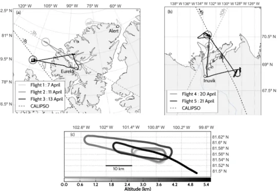
For the present study, five vertical profiles taken during five different flights were selected. These flights, whose trajecto-ries are shown in Fig. 3, were performed near Alert (82.5◦N, 62.3◦W), Eureka (80◦N, 86.1◦W) and Inuvik (68.3◦N, 133.7◦W) on 7, 11, 13, 20 and 21 April. All profiles were measured above snow-covered sea ice, which ensured that the surface was homogeneous contrary to flights performed above patches of snow and tundra or over areas of mixed sea ice and open water. All the investigated flights except 7 April were taken close to a track of the Cloud–Aerosol Lidar and Infrared Pathfinder Satellite Observations satellite (CALIPSO; Winker et al., 2003). Images taken by MODIS and the associated cloud products (Platnick et al., 2003) are also used to investigate cloud conditions above the aircraft. The five profiles were acquired in distinct atmospheric condi-tions, thus providing valuable samples of Arctic conditions in early spring. Flights from 7 to 13 April corresponded to typ-ical conditions of the high Arctic cold season, with low tem-peratures and a pronounced inversion, while the conditions near Inuvik were more representative of subarctic spring, with near-melting temperatures at the surface and denser clouds typically found in the mid-latitudes. Some ice clouds were encountered on 7 April flight, but the more typical polar optically thin ice cloud was probed on 13 April near Eureka. The three other flights exhibited clear sky conditions below the aircraft.
2.4 Radiative transfer simulations
One objective of the study was to perform radiative closure experiments by comparing FIRR measurements with radia-tive transfer simulations based on thermodynamical and mi-crophysical profiles recorded by the instruments aboard Polar 6. Here we used MODTRAN v.5.4 (Berk et al., 2005) to sim-ulate upwelling radiance at flight level. MODTRAN uses ab-sorption lines from HITRAN2013 and the MT-CKD 2.5 pa-rameterization of the water vapour continuum (Clough et al., 2005) that proved reliable in the Arctic (Fox et al., 2015). The spectral surface emissivity of snow was taken from Feld-man et al. (2014). Aerosols are approximated to the standard rural profile with a visibility of 23 km, which is consistent with the presence of Arctic haze during the campaign. Mul-tiple scattering is computed with DISORT (Stamnes et al., 1988) using 16 streams, and the band model is at 1 cm−1 spectral resolution. The model atmosphere has 75 levels from the surface to 30 km, with a resolution of 0.1 km near the sur-face stretching to 0.7 km at the top. In addition to radiances, MODTRAN was used to compute Jacobians through finite differences (Garand et al., 2001).
Temperature and humidity profiles were interpolated from the in situ measurements up to the maximum flying altitude. Above, they were taken from the closest ERA-Interim reanal-ysis (Dee et al., 2011), the latter being offset to ensure verti-cal continuity. Ozone profiles for the whole column were also taken from ERA-Interim. Snow surface temperature was ob-tained from the KT19 observations assuming a uniform spec-tral response of the instrument and a specspec-trally flat surface emissivity of 0.995 in the range 9.6–11.5 µm. All simulated clouds in this study are ice clouds defined by their optical thickness τ and particle effective diameter deff. Their single
scattering properties are calculated after the parameterization of Yang et al. (2005) for cirrus clouds. Cloud geometrical characteristics were deduced from the combination of in situ observations. Optical thickness and effective cloud particle diameter were not directly measured. For 7 April, both quan-tities were tuned to minimize the deviation from measure-ments. For 13 April, the particle effective diameter was taken from DARDAR satellite product (Delanoë and Hogan, 2010) and simulations were performed for various optical depths.
3 Results
In this section, the FIRR radiometric performances are first analyzed based on experiments performed on the ground and during one flight. The five case studies are then analyzed in detail and the vertical profiles of radiance acquired in clear sky and cloudy conditions are compared to radiative transfer simulations.
120º W 105º W 90º W 75º W 60º W 82.5º N 81º N 79.5º N 78º N 76.5º N 138º W 136º W134º W 132º W 130º W128º W126º W 70.5º N 69º N 67.5º N 102.6º W 102º W 101.4º W 100.8º W 100.2º W 99.6º W 81.62º N 81.6º N 81.58º N 81.56º N 81.54º N 81.52º N 81.5º N
Figure 3. Selected flight trajectories around (a) Eureka and (b) Inuvik. The circles indicate where the detailed vertical profiles were per-formed. CALIPSO tracks are also shown and hours indicate how much earlier (−) or later (+) the satellite flew over. (c) Detailed spiral ascent for the 11 April flight.
3.1 FIRR radiometric performances in airborne configuration
The FIRR performances were investigated through lab-oratory and ground-based experiments by Libois et al. (2016). They estimated a radiometric resolution around 0.015 W m−2sr−1and an absolute error of 0.02 W m−2sr−1, again slightly dependent on the channel considered. In air-borne configuration, the environmental conditions were more demanding due to cold ambient temperature and quick back-ground temperature variations. The FIRR performances for this specific setup are thus estimated from two experiments for which the environmental conditions were similar to nom-inal airborne operation, except the scene was more con-stant than in operation. Firstly, the brightness temperature of the snow surface below the aircraft was measured on Eu-reka runway on 12 April, while Polar 6 was parked without the propellers running. The ambient temperature was around −32◦C, the ABB was at −9.5◦C and the HBB at 20◦C. Sec-ondly, measurements taken on the closed rolling door just before landing on 11 April were analyzed. For this case, the ABB was at 15◦C and the HBB at 45◦C.
The experiment on snow consisted of 10 consecutive mea-surement sequences covering 30 min, so that 30 radiances were recorded for each spectral band. For all bands, the ra-diance increased continuously throughout the experiment, which was attributed to an increase of snow temperature. To remove this effect and focus on the resolution of the mea-surement only, the radiance series were first detrended, and
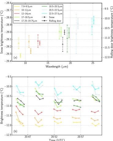
the standard deviation of the residual was then computed. The latter does not exceed 0.012 W m−2sr−1. The experi-ment performed on the rolling door consisted of five con-secutive sequences, and the standard deviation of the sig-nal was larger, reaching 0.021 W m−2sr−1. Figure 4a shows the corresponding brightness temperatures for both exper-iments, highlighting a temperature resolution around 0.1 K above snow and 0.2 K above the rolling door. Although the environmental conditions are slightly different in flight, these results provide a valuable reference and show that the instal-lation of the instrument in the aircraft did not affect its per-formances.
To further investigate the reduced radiometric resolution observed in flight, Fig. 4b shows the sequence of brightness temperatures recorded on the rolling door. A recurrent pat-tern is observed within a sequence of three consecutive mea-surements, with the first temperature generally larger than the following ones. We interpret this as the signature of fast and complex temperature variations of the skin temperature of the filters, which cannot be removed through the calibra-tion procedure. We attempted to use the numerous tempera-ture sensors embedded in the calibration enclosure and in the filter wheel to reconstruct the filters actual temperature, but this proved unsuccessful. Without any indication of whether any of the three consecutive points are the best, we simply conclude that this thermal instability results in an additive noise of approximate amplitude 0.2 K in worst conditions. This leaves room for future improvement of the instrument. The operational resolution of the FIRR nevertheless remains
10 15 20 25 Wavelength (µm) −29.4 −29.3 −29.2 −29.1 −29.0 −28.9 −28.8 −28.7 −28.6 Sno w brightness temp erature ( ◦C) 7.9–9.5µm 10–12µm 12–14µm 17–18.5µm 17.25–19.75µm 18.5–20.5µm 20.5–22.5µm 22.5–27.5µm Snow Rolling door −12.0 −11.5 −11.0 −10.5 −10.0 −9.5 Rolling do or brightness temp erature ( ◦C) (a) 20:47 20:52 20:57 Time (UTC) −12.5 −12.0 −11.5 −11.0 −10.5 −10.0 −9.5 Brightness temp erature ( ◦C) (b)
Figure 4. (a) Mean and standard deviations (error bars) of the de-trended brightness temperatures along 10 sequences (i.e. 30 consec-utive measurements) for measurements taken on snow on 12 April (15:10–15:42 UTC) and along 5 sequences on the rolling door on 11 April (21:45–22:00 UTC). For 12 April, THBB=20◦C and TABB= −9.5◦C. For 11 April, THBB=45◦C and TABB=15◦C. (b) Temporal evolution of brightness temperature for the five se-quences acquired on the closed rolling door on 11 April. The 30– 50 µm band is not shown because it suffered from the temperature stability problem mentioned in Sect. 2.2.1.
well below 0.5 K, which is still satisfactory and comparable to temperature measurements performed aboard Polar 6. This issue had not been noticed by Libois et al. (2016), most likely because in their study ambient temperature was closer to the internal temperature of the FIRR, limiting the range of filter temperature variations.
3.2 Clear sky cases
The profiles on 11, 20 and 21 April were all taken in clear sky conditions, but the total columns of water vapour were very different. These flights are specifically used to investi-gate the impact of temperature and humidity variations on the measured profiles of spectral radiances.
3.2.1 11 April
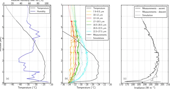
The ascent started at 19:02 and at 19:52 UTC Polar 6 reached the maximum altitude of 5.56 km, where it stayed for 4 min. On its way up it also levelled at 2.75 km for 7 min. The surface temperature retrieved from the KT19 was −32.6◦C while a maximum of −24◦C was observed in the atmo-spheric temperature profile between 1 to 2 km (Fig. 5a). The whole atmosphere was undersaturated with respect to ice, ex-cept near the surface. The total column water vapour was 1.5 mm, with 1.4 mm below 5.56 km. No clouds were ob-served and the Aqua MODIS image taken at 18:45 UTC shows that no clouds were present above either. FIRR bright-ness temperature profiles show interesting features (Fig. 5b), with the temperature inversion more obvious for the longer wavelengths for which the atmosphere is more opaque. To further illustrate this differential sensitivity to the tempera-ture profile, Fig. 6 shows the penetration depth of each chan-nel as a function of altitude. The chanchan-nels that penetrate the least are sensitive to the conditions closest below the aircraft. As expected, the brightness temperature in the highly trans-parent atmospheric window (10–12 µm) is essentially con-stant with height since it is insensitive to the properties of the atmosphere. The slight increase of 0.5 K from the surface to the top is also observed in KT19 records and is probably the signature of surface temperature variations. The 17–18.5 µm and 18.5–20.5 µm profiles are very similar, implying relative redundancy between these two channels. The very distinct behaviours of window and FIR channels still result in nearly similar brightness temperatures at the top of the profile. This feature, typical of the Arctic, highlights the complexity of probing from space an atmosphere with a strong tempera-ture inversion. The peaks in the shorter wavelengths channels around 4 km were found to visually correspond to variations of sea ice characteristics. They could be due to thinner and warmer sea ice or finer snow with higher emissivity (Chen et al., 2014). Since all individual measurements were used, the vertical resolution is close to 200 m. However, the in-stability along three measurements is noticeable, e.g. for the 18.5–20.5 µm channel below 2 km. Besides this instrumen-tal noise, part of the observed signal variation might be due to horizontal inhomogeneity, especially when the aircraft roll reaches up to 20◦in turns.
The vertical profile of upwelling broadband LW radia-tion also highlights the temperature inversion, with a max-imum around 2 km, similar to the FIR channels of the FIRR (Fig. 5c). LW fluxes have been simulated with MODTRAN and are also shown. The simulated and measured profiles are in close agreement above 2 km, with a root mean square devi-ation (RMSD) of 0.35 W m−2. Such a value is consistent with the accuracy provided by the manufacturer and the absolute uncertainty of 2 W m−2suggested by Marty (2003) for such sensors. This is very satisfactory for a sensor sensitive only up to 42 µm while a significant part of the energy lies beyond, and considering that the calibration was done above 2◦C.
−50 −45 −40 −35 −30 −25 −20 Temperature (◦C) 0 1 2 3 4 5 6 7 Altitude (km) 0 20 40 60 80 100
Relative humidity over ice (%)
(a) Temperature Humidity −36 −34 −32 −30 −28 −26 −24 −22 −20 Temperature (◦C) 0 1 2 3 4 5 6 7 (b) Temperature 7.9–9.5 µm 10–12 µm 12–14 µm 17–18.5 µm 18.5–20.5 µm 20.5–22.5 µm 22.5–27.5 µm Measurements Simulations 170 175 180 185 190 195 200 205 210 Irradiance (W m−2) (c) Measurements - ascent Measurements - descent Simulation
Figure 5. Vertical profiles of (a) temperature and relative humidity measured by in situ probes, (b) FIRR brightness temperatures and (c) upwelling broadband LW irradiance measured by the CGR-4 pyrgeometer for 11 April flight. The ascent portion correspond to the vertical profile and the descent portion shows the measurements taken 20 min prior to the ascent. The simulated FIRR brightness temperatures and LW irradiance are also shown. The 17.25–19.75 µm band is not shown because it overlaps with others. The dashed lines in panel (a) correspond to the ERA-Interim profiles used for the simulations above maximum flying altitude.
0 1 2 3 4 5 6 Penetration depth (km) 0 1 2 3 4 5 6 Altitude (km) 7.9–9.5 µm 10–12 µm 12–14 µm 17–18.5 µm 18.5–20.5 µm 20.5–22.5 µm 22.5–27.5 µm
Figure 6. Penetration depth of each channel as a function of flying altitude for the 11 April flight. Penetration depth is defined as the downward distance from the plane such that the broadband trans-mittance in this channel reaches 75 %.
This agreement gives high confidence in the atmospheric profile measurements, as well as in the aerosols modelled in MODTRAN, because errors in aerosol profiles could result in discrepancies of several W m−2(Sauvage et al., 1999). Re-garding the upper extrapolated part of the atmosphere, com-parisons of measured and simulated downwelling LW fluxes (not shown) are also in reasonably good agreement, which gives confidence in the ERA-Interim fields. Close to the sur-face, measurements show an unexpected peaked minimum. Although the origin of this peak is not fully understood,
we believe this is an instrumental artifact resulting from the strong temperature gradient near the surface and the sen-sor not being at thermal equilibrium (Ehrlich and Wendisch, 2015). This hypothesis is supported by the fact that data taken on the way down just before starting the ascent show a peak in the opposite direction.
MODTRAN was also used to simulate FIRR brightness temperatures (Fig. 5b). The measured profiles for all chan-nels are well simulated, with a mean bias and RMSD below 0.2 K. The agreement in the window bands confirms that no clouds were present below the aircraft. FIR simulations pro-vide strong validation of the radiative transfer model, result-ing in a satisfactory radiative closure in clear sky conditions. The spectral brightness temperatures are compared at the two altitudes where multiple measurements were taken. Figure 7 shows the average measured brightness temperatures at 2.75 and 5.56 km and the corresponding simulations. The spectral RMSD is below 0.15 K at both altitudes, which is very sat-isfying, given that MODTRAN user’s manual suggests that the model accuracy is 1 K. The variability of the measure-ments at each step is below 0.4 K, which is consistent with the results of Fig. 4b. In addition, most deviations between observations and simulations are within the range of uncer-tainties due to unceruncer-tainties of the temperature and relative humidity measurements.
Overall, the simulations reproduce well the observations, which validates to some extent the radiative transfer code configuration and the implemented snow emissivity. How-ever, such measurements can hardly be used for model im-provement. As pointed out by Mlynczak et al. (2016), the inherent uncertainties related to the atmospheric
measure-10 15 20 25 Wavelength (µm) −34 −33 −32 −31 −30 −29 −28 −27 Brightness temp erature ( ◦C) Measurements - 2.75 km Measurements - 5.56 km Simulations - 2.75 km Simulations - 5.56 km
Figure 7. Measured and simulated spectral brightness temperatures at the two altitudes where Polar 6 levelled during 11 April flight. At both levels four consecutive measurements were taken. Their means and ranges are indicated by the circles and error bars, respectively. The shaded areas indicate the uncertainties in the simulations due to uncertainties on the measured temperature and relative humidity profiles, namely 0.3 K and 2.5 %.
ments and radiative transfer parameterization likely exceed the FIRR measurements uncertainties. Agreement is thus sat-isfactory and encouraging for the performances of the instru-ment but does not give further indications about the quality of the model inputs and parameterizations.
3.2.2 20 and 21 April
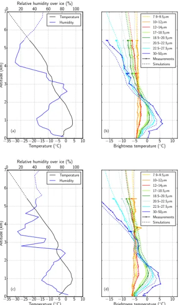
Both flights took place in the vicinity of Inuvik and showed relatively warm conditions and above freezing temperatures at the inversion level (Fig. 8a and c). The cloud probes suggested that no clouds were present, which is consistent with the relative humidity profiles. For 20 April flight, a moist layer typical of long range transport was found, which peaked near 2.5 km at about 85 % humidity with respect to water. Above 3.5 km, this layer was topped with drier air associated with weak air subsidence. Above 3.8 km, the air was very whitish, and the FSSP-300 and sun photometer in-dicated increased level of aerosols. Likewise, SP2 measure-ments showed increasing amounts of black carbon with alti-tude, exceeding 0.1 µg m−3, which is indicative of a polluted air mass. Similar conditions were encountered on 21 April, except that the polluted layer was located above 2.6 km, which again coincided with a drop of relative humidity. Sun-photometer data suggest the presence of high-altitude clouds with optical depth around 0.2, but characterized by large vari-ability. Those clouds were not accounted for in the simula-tions.
The vertical profiles of brightness temperatures are simi-lar for both flights (Fig. 8b and d). Again, the window chan-nels show very weak variations, which is characteristic of clear sky conditions. On the contrary, FIR channels are char-acterized by rapid variations near the surface and a larger
−35−30−25−20−15−10 −5 0 5 10 Temperature (◦C) 0 1 2 3 4 5 6 7 Altitude (km) 0 20 40 60 80 100 Relative humidity over ice (%)
(a) Temperature Humidity −15 −10 −5 0 5 10 Brightness temperature (◦C) (b) 7.9–9.5µm 10–12µm 12–14µm 17–18.5µm 18.5–20.5µm 20.5–22.5µm 22.5–27.5µm 30–50µm Measurements Simulations −35−30−25−20−15−10 −5 0 5 10 Temperature (◦C) 0 1 2 3 4 5 6 7 Altitude (km) 0 20 40 60 80 100 Relative humidity over ice (%)
(c) Temperature Humidity −15 −10 −5 0 5 10 Brightness temperature (◦C) (d) 7.9–9.5µm 10–12µm 12–14µm 17–18.5µm 18.5–20.5µm 20.5–22.5µm 22.5–27.5µm 30–50µm Measurements Simulations
Figure 8. Vertical profiles of temperature and relative humidity for (a) 20 April and (c) 21 April flights. Measured and simulated FIRR brightness temperatures for (b) 20 April and (d) 21 April flights. The dashed lines in panels (a) and (c) correspond to the ERA-Interim profiles used for the simulations above maximum flying al-titude.
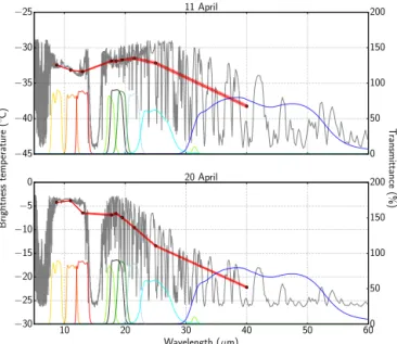
lapse rate at higher altitude compared to the 11 April flight. These features are due to a sharper temperature inversion and a reduced transparency of the atmosphere (the column water vapour below 5.4 km are 10.3 and 10.5 mm, respec-tively). The difference between the conditions encountered on 11 and 20 April is further illustrated in Fig. 9. It shows the high spectral resolution brightness temperature simulated by MODTRAN at 6 km altitude for both flights and the corre-sponding simulated FIRR spectral signatures. This highlights the greater transparency of the atmosphere in the FIR for the 11 April. The peak observed at 3.8 km on 21 April corre-sponds to measurements over open water, as shown by a
pic-−45 −40 −35 −30 −25 11 April 10 20 30 40 50 60 Wavelength (µm) −30 −25 −20 −15 −10 −5 0 Brightness temp erature ( ◦C) T ransmittance (%) 20 April 0 50 100 150 200 0 50 100 150 200
Figure 9. High spectral resolution brightness temperatures simu-lated with MODTRAN for the 11 and 20 April flights at 6 km al-titude. FIRR filters transmittances are also shown, as well as the simulated FIRR spectral signatures. The red shaded areas indicate the uncertainties in the simulations due to uncertainties on the mea-sured temperature and relative humidity profiles.
ture taken concomitantly (Fig. 10). More generally, since Po-lar 6 approximately flew at 75 m s−1, a single measurement of 0.8 s spanned 60 m at the surface. Similarly, a typical roll of 10◦during the spiral corresponds to 1 km deviation at the surface when flying at 6 km. This could generate noise if the surface was not homogeneous at this scale, which was the case at the interface between the sea ice and open water.
The simulated brightness temperatures in the atmospheric window are in good agreement with observations, but devi-ations exceeding measurement uncertainties are found in the FIR channels for the upper part of the profile. The largest discrepancies are obtained in the 30–50 µm band, with mea-surements being approximately 1.5 K warmer than the sim-ulations. In fact, the air transmittance in this channel is so low that a significant part of the signal comes from the air contained in the 56 cm long chimney just below the instru-ment rather than from the atmosphere below. This artifact was noticed by Mlynczak et al. (2016). Using their correc-tion (Eq. 1), we find that air at −5◦C and 50 % relative hu-midity in the chimney can increase the apparent brightness temperature at 5 km altitude by 1.5 K in the 30–50 µm band, while the deviation does not exceed 0.3 K for the other chan-nels. For this reason, the data in the 30–50 µm band are not reliable and are not shown in the rest of the paper. This is not critical in this study because at the flying altitude this band essentially probes local temperature. On the contrary, it is expected to be very valuable from a satellite view, where it should provide information about water vapour and clouds at the very top of the troposphere. The consistent positive bias
of the simulations in the other FIR channels is more puzzling, especially because it is observed in both flights. Several fac-tors could explain such discrepancies. Inaccuracies in the wa-ter vapour continuum are ruled out because recent studies have shown uncertainties below 10 % (Liuzzi et al., 2014; Fox et al., 2015), largely insufficient to explain such differ-ences. Errors in water vapour measurements are also unlikely because independent measurements taken by distinct instru-ments aboard Polar 6 show differences less than 20 %, while only an increase larger than 50 % could explain the observed differences. In addition, water vapour measurements along track did not show significant variability, so that spatial vari-ability of water vapour can be ruled out. Only the incursion of a wet air mass below the aircraft before the end of the as-cent could explain such a discrepancy between observations and simulations. In such case the water vapour profile used in the simulation would not correspond to the actual profile at the time of the measurement, but this is unlikely given that it was observed on two different flights. Adding an optically thin cloud between 6 and 9 km altitude did not improve the simulations either. Given the verified accuracy of the FIRR, we hypothesize that the differences are the consequence of the observed haze layer. This is in line with the significant radiative signature in the IR shown by Ritter et al. (2005) for similar aerosol optical depths as those experienced in these two flights. The fact that the window channels are not im-pacted remains unanswered, though. This might be due to the specific nature of the wet aerosols forming the haze layer, which should have a signature similar to water vapour in the FIR. This question is left to future work, where hyperspec-tral measurements would certainly help investigating the de-tailed response. It should nevertheless be borne in mind that in these particular cases the greenhouse effect is underesti-mated in MODTRAN simulations, which can lead to signif-icant deviations on the atmospheric and surface energy bud-gets.
3.3 Cloudy cases
Flights performed on 7 and 13 April are used to assess the radiative impact of optically thin ice clouds in the FIR. They also highlight the difficulty to compare in situ observations to radiative transfer simulations due to high variability of the cloud microphysics.
3.3.1 7 April
During this flight west of Alert, singular atmospheric condi-tions were encountered. Near the surface, a saturated layer was found up to 1.1 km where a cloud was present, as de-tected by the Nevzorov and 2D-C probes. Another cloud was found above 4 km, which extended up to the maximum fly-ing altitude of 6 km. In between, the atmosphere was very dry. The temperature profile had a complex signature near the surface, where a double temperature inversion was observed
Figure 10. Downward picture of the surface taken on 21 April at 17:35 UTC and 3.8 km altitude. The 300 m diameter circles depict the FIRR footprint at the surface for a single 0.8 s measurement. Plain line circles indicate the relative positions of the aircraft when the measurement is performed on the first filter, and dashed circles when performed on the last filter (flight direction is to the right). It takes approximately 20 s to measure all nine filters and another 20 s to come back to the position of the first filter.
(Fig. 11), probably due to radiative cooling at top of the near-surface cloud. Observed FIRR brightness temperatures are consistent with the atmospheric profile. In the clear sky re-gion, the profiles are similar to that of 11 April. In clouds, brightness temperature varies more rapidly with altitude, as a consequence of increased absorption and scattering in all channels. Consequently, all brightness temperatures samples at 5.7 km are contained in a narrow 1.5 K range.
Since CALIPSO does not cover such high latitudes, we do not have supplementary information regarding the clouds properties. The profile of relative humidity suggests that the cloud was initiated above 5 km in saturated air with respect to ice, and below ice particles were precipitating without sat-urating the air. For the MODTRAN simulations, the parti-cle effective diameter was set to 75 µm, with relatively large particles consistently seen by the 2D-C probe but missed by the FSSP-300. We then tuned the optical depth to 0.5 for the near-surface cloud layer and 1.0 for the upper layer cloud. This set of cloud properties produces brightness temperatures profiles in agreement with the measurements. The brightness temperature difference between 7.9–9.5 µm and 10–12 µm channels is larger in the model than in the observations yet, which suggests an imperfect definition of aerosol and haze profiles.
3.3.2 13 April
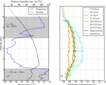
The best case of optically thin ice cloud was observed during 13 April flight. A vertical profile was taken during the de-scent between 18:15 and 19:12 UTC. The temperature pro-file was fairly typical of Arctic winter conditions, with an
−50 −45 −40 −35 −30 −25 −20 −15 −10 Temperature (◦C) 0 1 2 3 4 5 6 7 Altitude (km) 0 20 40 60 80 100 120
Relative humidity over ice (%)
(a) τ = 0.8 deff= 50µm τ = 0.4,deff= 50µm Temperature Humidity −30 −28 −26 −24 −22 −20 −18 −16 Brightness temperature (◦C) (b) 7.9–9.5µm 10–12µm 12–14µm 17–18.5µm 18.5–20.5µm 20.5–22.5µm 22.5–27.5µm Measurements Simulations
Figure 11. Vertical profiles of (a) temperature and relative humid-ity and (b) measured and simulated FIRR brightness temperatures for 7 April flight. Shaded areas in panel (a) indicate the presence of clouds. The optical thickness and particle effective diameter used for the simulations are also indicated. The dashed lines correspond to the ERA-Interim profiles used for the simulations above maxi-mum flying altitude.
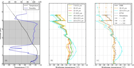
inversion at 1.3 km and surface temperature around −25◦C (Fig. 12a). A tenuous cloud layer was found below 1 km and a much thicker cloud was observed between 2.2 and 5 km according to the combination of 2D-C and FSSP-300 probes. These two instruments, along with the relative humidity pro-file, suggest that ice particles formed above 3 km but large precipitating crystals were observed down to 2.2 km. This cloud is similar to a TIC-2B type from the classification of Grenier et al. (2009). The FIRR brightness temperatures are characterized by high vertical variability, especially above 3 km (Fig. 12b). This variability is identical for all bands, suggesting that it is due to actual scene variations. The excel-lent match between KT19 measurements and the 10–12 µm channel confirms that observed variations are not instrumen-tal artifacts (Fig. 12c). Instead, they are attributed to cloud horizontal variability. This hypothesis is supported by the sun-photometer data that show highly varying optical depth above the aircraft as well.
Since the aircraft is flying in quasi-spirals of 10 km di-ameter, any cloud variability below this scale results in sig-nal variability on the vertical profile. Down-looking pic-tures taken on Polar 6 show that above 3 km, surface fea-tures were intermittently visible, meaning that cloud opti-cal depth varied substantially along the flight path. Attempt-ing to reproduce the measured brightness temperature pro-files with a 1-D model was impractical. Instead, several MODTRAN simulations were performed for various opti-cal depths. For these simulations, particle effective diame-ter was set to 120 µm, consistently with DARDAR product
−50 −45 −40 −35 −30 −25 −20 −15 Temperature (◦C) 0 1 2 3 4 5 6 7 Altitude (km) 0 20 40 60 80 100 120
Relative humidity over ice (%)
(a) Temperature Humidity −32 −30 −28 −26 −24 −22 −20 −18 −16 −14 Brightness temperature (◦C) (b) 7.9–9.5 µm 10–12 µm 12–14 µm 17–18.5 µm 18.5–20.5 µm 20.5–22.5 µm 22.5–27.5 µm −32 −30 −28 −26 −24 −22 −20 −18 −16 −14 Brightness temperature (◦C) (c) FIRR 10–12 µm 22.5–27.5 µm KT19 Simulations τ = 0.5 τ = 2.0 τ = 5.0
Figure 12. Vertical profiles of (a) temperature and relative humidity and (b) FIRR brightness temperatures for 13 April flight. In panel (a), the shaded areas indicate the presence of clouds and the dashed lines correspond to the ERA-Interim profiles used for the simulations above maximum flying altitude. Panel (c) shows measured and simulated brightness temperatures for two FIRR bands and various optical depths of the upper cloud. KT19 temperatures are shown as well for comparison to FIRR 10–12 µm channel.
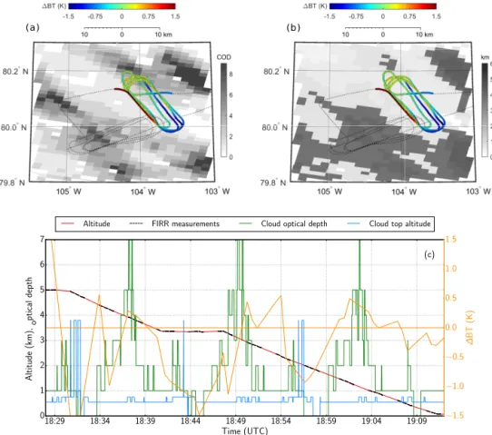
corresponding to a CALIPSO overpass at 16:10 UTC. The near-surface cloud optical depth was set to 0.07, while the upper cloud optical depth τ was varied from 0.5 to 5 in the calculations. Figure 12c shows that the range 0.5–5 repro-duces quite well the observed variability of brightness tem-perature. We infer that at small scale cloud variability is ex-tremely high, which is unexpected from satellite data on the large scale for this type of cloud (Grenier et al., 2009). To further investigate the spatial variability, MODIS cloud prod-ucts at 18:09 UTC were analyzed. In particular, the cloud op-tical depth and cloud top altitude, shown in Fig. 13, are very instructive. At the scale of Polar 6 spiral, the cloud optical depth is indeed highly variable, ranging from nearly clear sky to values exceeding 5. The cloud top altitude also shows that the probed cloud with top at 5 km was very localized in the most southeastern section of the spiral. Interestingly, these spatial features are consistent with FIRR observations. In fact, the difference between the temperature measured by the 10–12 µm channel and the simulation with τ = 2 (indicated by the colour of the trajectory in Figs. 13a and b) is minimum near the area corresponding to the high-altitude cloud, which suggests that the cloud there has an optical depth larger than 2. The difference is larger elsewhere, meaning that FIRR senses warmer temperatures corresponding to either a thin-ner or lower cloud. The variations of the brightness tempera-ture difference are more evident in Fig. 13c, which shows the time series of the difference along with the MODIS estimates of cloud characteristics. Observed FIRR spatial variability is thus consistent with the presence of a cloud of optical depth around 4 in the southeastern bound of the trajectory that ex-tends up to 5 km. Elsewhere on the trajectory the atmosphere ranges from clear to low-altitude clouds. The latter also seem
to be variable, resulting in slight variations of brightness tem-perature in the window channels near the surface. This case illustrates the complexity of atmospheric radiative transfer in heterogeneous conditions. It also shows that the FIRR is responding consistently with variations in clouds conditions from a nadir view similar to a satellite view.
4 Discussion
The five case studies investigated in the previous section pro-vided a valuable insight on FIRR performances from an air-borne nadir configuration and on the FIR characteristics of the Arctic atmosphere in clear and cloudy conditions. To fur-ther explore the dependence of FIRR measurements on at-mospheric profiles, a series of radiative transfer simulations are performed. The results are then discussed in the frame-work of TICFIRE, with the intent to improve the data quality in future similar airborne campaigns.
4.1 Sensitivity to temperature, humidity and cloud properties
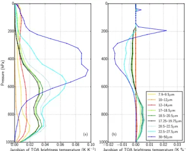
In order to extend the interpretation of the data acquired dur-ing the NETCARE campaign, the Jacobians of the top of at-mosphere (TOA) brightness temperature with respect to tem-perature and humidity were computed for 11 April simula-tions (Fig. 14). The Jacobian at a given atmospheric level is the difference in simulated TOA brightness temperature resulting from an increase of 1 K (1 % specific humidity) of the temperature (relative humidity) at this level. The tempera-ture Jacobians show that the 30–50 µm channel is mostly sen-sitive to atmospheric layers below 500 hPa (above ∼ 5 km),
(a) (b) 18:29 18:34 18:39 18:44 18:49 18:54 18:59 19:04 19:09 Time (UTC) 0 1 2 3 4 5 6 7 Altitude (km), optical depth −1.5 −1.0 −0.5 0.0 0.5 1.0 1.5 ∆ BT (K) (c)
Altitude FIRR measurements Cloud optical depth Cloud top altitude
Figure 13. (a) Optical depth at 1.24 µm and (b) cloud top altitude derived from MODIS observations at the beginning of the profile on 13 April (18:09 UTC). Polar 6 trajectory is highlighted, with the colour corresponding to the difference between measured and simulated (τ = 2) brightness temperatures for the 10–12 µm channel. Blue suggests the actual optical depth is larger than 2 while red suggests it is less. (c) Difference between measured and simulated (τ = 2) brightness temperatures for the 10–12 µm channel as a function of time, along with flight altitude and MODIS estimates of cloud optical depth and cloud top altitude. Black dots indicate when FIRR spectral measurements are actually performed.
which explains why this channel was not very useful at lower altitude during the campaign. The shorter FIR wavelengths are sensitive to lower layers of the atmosphere, and window channels are almost insensitive to the atmosphere tempera-ture. These Jacobians also suggest that the three channels between 17 and 20 µm are very similar, making them some-what redundant in such atmospheric conditions. Comparing the absolute values of the Jacobians to the FIRR resolution gives a lower estimate of the vertical resolution the FIRR could reach for profiles retrieval applications. Given the ra-diometric resolution of the FIRR is about 0.2 K, temperature variations of 0.2 K are detectable with a vertical resolution of 100 to 200 hPa in FIR bands. Regarding the FIRR sensi-tivity to variations in relative humidity, Fig. 14b shows that the 30–50 µm band is the most sensitive, as expected due to the water vapour absorption spectrum. Humidity variations of 5 % for a 100 hPa thick layer above 600 hPa should pro-duce a detectable signal for all FIR bands, highlighting the potential of the FIRR for probing humidity profiles in such cold and dry conditions. Note that the Jacobians are positive
around the temperature inversion, which is a feature typical of polar conditions. Negative values are consistent with the fact that increasing water vapour increases the greenhouse effect due to the atmosphere and hence decreases radiation at TOA.
To complement this sensitivity analysis, an ice cloud was inserted between 2 and 6 km in the same atmosphere, and the relative humidity with respect to ice was correspond-ingly set to 100 %. Starting from a reference cloud, its op-tical depth and particle effective diameter were varied. Fig-ure 15 shows that TOA FIR brightness temperatFig-ures are very sensitive to cloud optical depth, with variations up to 5 K between clear sky conditions and τ = 5. The FIRR resolu-tion approximately converts into a 0.2 resoluresolu-tion in terms of optical depth. The same exercise with varying optical depth shows that for small particles FIR channels are very sensitive to particle size. However, the sensitivity quickly decreases for larger sizes, which is consistent with the findings of Yang et al. (2003) and Baran (2007), who suggested a sensitivity up to 100 µm effective dimensions. This sensitivity is directly
0.00 0.02 0.04 0.06 0.08 0.10
Jacobian of TOA brightness temperature (K K−1)
0 200 400 600 800 1000 Pressure (hP a) (a) −0.02 −0.01 0.00 0.01 0.02 0.03
Jacobian of TOA brightness temperature (K %−1)
0 200 400 600 800 1000 (b) 7.9–9.5µm 10–12µm 12–14µm 17–18.5µm 18.5–20.5µm 17.25–19.75µm 20.5–22.5µm 22.5–27.5µm 30–50µm
Figure 14. (a) Temperature and (b) humidity Jacobians for the TOA brightness temperature for 11 April atmospheric profile. For humid-ity, variations are in % of the specific humidity.
related to the crystal shape and size distribution assumed for this study, which correspond to cirrus clouds. Although the results above are qualitatively robust, using another ice cloud parameterization could have resulted in different val-ues (e.g. Baran, 2007). In particular, Arctic clouds character-ized by rapid crystal growth in high supersaturation condi-tions may actually have shallower particle size distribucondi-tions (Jouan et al., 2012) and exhibit more sensitivity to particle size.
4.2 Recommendations for future operation
The preceding results are now discussed in the framework of planning the TICFIRE satellite mission and in view of future airborne campaigns with the FIRR or similar instruments. First of all, one advantage of using uncooled microbolome-ters is the possibility to have an imager, as will be the case for TICFIRE. In this study, the FIRR was not used as an im-ager, though, because it has a much narrower field of view than TICFIRE satellite configuration. However, it is worth exploring how the accuracy of the measurements would de-cay if spatial averaging were skipped. To this end, the spec-tral brightness temperature shown in Fig. 7 is computed again from FIRR measurements, except that spatial averaging is made on 1 (no averaging), 4, 9 or 193 pixels. Nominal data processing is optimized for 193 pixels and could not be ap-plied to a single pixel (Libois et al., 2016), so that the proce-dure was slightly changed to ensure that the same calibration is applied independently of the number of pixels averaged. The results are shown in Fig. 16. As expected, spatial av-eraging improves the repeatability of the measurement, but averaging over 9 pixels already provides a resolution close to 193 pixels. The absolute values are very consistent, with
10 20 30 40 50 60 Wavelength (µm) −3 −2 −1 0 1 2 Brightness temp erature difference (K) (a) τ = 0.1 τ = 0.2 τ = 0.5 τ = 1.0 τ = 1.5 τ = 2.5 τ = 3.0 τ = 4.0 τ = 5.0 10 20 30 40 50 60 Wavelength (µm) −1.0 −0.5 0.0 0.5 1.0 1.5 2.0 Brightness temp erature difference (K) (b) deff= 5 µm deff= 10 µm deff= 20 µm deff= 30 µm deff= 50 µm deff= 100 µm deff= 150 µm deff= 200 µm
Figure 15. TOA brightness temperature differences between var-ious clouds and the reference with τ = 2 (τ = 3 for panel b) and deff=80 µm. Panel (a) is for varying optical depth while panel (b) is for varying particle effective diameter.
differences less than 0.5 K if more than 1 pixel are used. The remaining differences can be attributed to instrument errors, but scene spatial heterogeneities cannot be ruled out. This suggests that the present study is relevant to verify the perfor-mances of the future TICFIRE satellite instrument, the pre-cision of which could be increased through spatial averaging over neighbour pixels.
It is worth pointing out that the NETCARE campaign was not dedicated solely to radiation measurements. Probing ice clouds was one of the objectives, but not the only one. In addition, few clouds were encountered during the campaign and days with too many clouds prevented aircraft operations for safety reasons. Overall the dataset is still modest and fur-ther campaigns in the Arctic winter remain necessary, in par-ticular to complete a radiative closure in cloudy conditions, which was not possible here due to lack of quantitative in-formation about clouds properties. Such campaigns should be dedicated to the radiative properties of ice clouds in or-der to maximize the scientific success of this research topic (e.g. CIRCCREX; Fox, 2015). During the NETCARE cam-paign, the FIRR was supposed to have a zenith view to al-low net fluxes computation and associated cooling rates, but shortly before the campaign started this configuration proved to be incompatible in terms of safety. In the future,
com-10 15 20 25 Wavelength (µm) −34 −33 −32 −31 −30 Brightness temp erature ( ◦C) 1 pixels 4 pixels 9 pixels 193 pixels
Figure 16. FIRR spectral brightness temperatures at 5.56 km as in Fig. 7, except that measurements were averaged over a varying number of pixels, from 1 to 193. Error bars indicate measurement variability along four consecutive measurements. For each spectral band the four corresponding error bars are slightly displaced hori-zontally for sake of clarity.
bining nadir and zenith views as in Mlynczak et al. (2011) would be extremely beneficial to the understanding of the atmospheric radiative budget in the FIR. From the FIRR per-spective, we noticed that upgrading the current instrument radiometric resolution is essential to further constrain radia-tive transfer simulations and cloud properties retrievals. This can be achieved by improving the environmental conditions of the FIRR within the aircraft, paying more attention to tem-perature stability. Adding an insulating window to prevent air circulation around the instrument or increasing the pressure inside the instrument to ensure constant outflow from the air-craft would minimize temperature variations. Note that these recommendations are linked to the fact that Polar 6 cabin is unpressurized and other constraints should be thought of in the case of a pressurized aircraft. Complementary zenith and nadir observations would also be extremely valuable in order to compute cooling rates and sample the whole atmospheric profile.
At the instrument level, the FIRR is the first prototype and improvements are expected from technological develop-ments of uncooled microbolometers, but optimization in the analogical–numerical converter and absence of the detector window in space could already increase the current resolu-tion by a factor of 3 to 5. Likewise, increasing acquisiresolu-tion rate by using a faster filter wheel and scene selection motor would reduce the acquisition time of a sequence by one order of magnitude, thus limiting temperature variations in between calibrations. It would also ensure that measurements in all channels are taken on the same target, which was not always the case during the campaign above leads or through highly heterogeneous ice clouds. Such technical developments are already considered and will be mandatory for the satellite version of the instrument which requires acquisition times around 1 s for a complete scene sequence.
5 Conclusions
The first airborne campaign of the FIRR took place in the Arctic in the framework of the NETCARE aircraft campaign. It was a great opportunity to study the radiative properties of the early spring Arctic atmosphere, and it highlighted the im-portance of water vapour and ice clouds in this remote envi-ronment. Vertical profiles of brightness temperature acquired in clear sky and cloudy conditions provided a strong obser-vational constraint on the radiative properties. At the same time, they increased the limited amount of observations avail-able in the far-infrared, especially in such remote regions. These observations also provided valuable knowledge about the FIRR instrument, which can be used to improve operation and development in view of the TICFIRE satellite mission. This campaign showed that the current state-of-the-art radia-tive transfer models are well suited for the Arctic and confirm that instrument resolution is better than the uncertainties in-herent to the radiative transfer formulation and input observa-tions. They also show that aerosols can significantly impact the radiative budget of the atmosphere, thus implying that a detailed characterization of the aerosols and haze is nec-essary to refine radiative closure experiments. Although the FIRR behaved very well during the campaign with respect to its nominal performances, the latter could be improved for accurate retrievals of atmospheric and cloud characteristics. The campaign proved that ice clouds in the Arctic are hard to probe, as much for reasons of safety as for their complex-ity and their high heterogenecomplex-ity. As a consequence, measured ice clouds spectral signature could not be compared to sim-ulations with sufficiently well-constrained cloud properties. Such airborne campaigns should be replicated to improve our understanding of ice cloud formation and radiative properties in polar regions. Accordingly, they should be dedicated to ra-diation and combine cloud microphysical observations with various radiation sensors. Such studies are necessary to con-tinue improving our knowledge of ice cloud formation and its parameterization in numerical weather prediction and cli-mate models.
6 Data availability
All NETCARE data will be made public after the end of the project (http://www.netcare-project.ca). In the meantime, ac-cess can be granted by contacting the project manager Bob Christensen ([email protected]). The FIRR data used in this study are available upon request from the au-thors ([email protected]). Requests for ac-cess to AWI data should be sent to Martin Gehrmann ([email protected]). The CALIPSO and DARDAR prod-ucts were obtained from the ICARE Data Center (http:// www.icare.univ-lille1.fr/). MODIS data were obtained from LAADS (https://ladsweb.nascom.nasa.gov/).