Agile quadrotor maneuvering using
tensor-decomposition-based globally optimal control
and onboard visual-inertial estimation
by
Fabian Riether
B.S., Engineering Cybernetics (2013)
University of Stuttgart
Submitted to the Department of Mechanical Engineering
in partial fulfillment of the requirements for the degree of
Master of Science in Mechanical Engineering
at the
MASSACHUSETTS INSTITUTE OF TECHNOLOGY
September 2016
c
○
Massachusetts Institute of Technology 2016. All rights reserved.
Author . . . .
Department of Mechanical Engineering
August 01, 2016
Certified by. . . .
Sertac Karaman
Associate Professor of Aeronautics and Astronautics
Thesis Supervisor
Certified by. . . .
John Leonard
Professor of Mechanical and Ocean Engineering
Mechanical Engineering Faculty Thesis Reader
Accepted by . . . .
Rohan Abeyaratne
Quentin Berg Professor of Mechanics
Chairman, Department Committee on Graduate Theses
Agile quadrotor maneuvering using
tensor-decomposition-based globally optimal control
and onboard visual-inertial estimation
by
Fabian Riether
Submitted to the Department of Mechanical Engineering on August 01, 2016, in partial fulfillment of the
requirements for the degree of
Master of Science in Mechanical Engineering
Abstract
Over the last few years, quadrotors have become increasingly popular amongst re-searchers and hobbyist. Although tremendous progress has been made towards mak-ing drones autonomous, advanced capabilities, such as aggressive maneuvermak-ing and visual perception, are still confined to either laboratory environments with motion capture systems or drone platforms with large size, weight, and power requirements. We identify two recent developments that may help address these shortcomings. On the one hand, new embedded high-performance computers equipped with pow-erful Graphics Processor Units (GPUs). These computers enable real-time onboard processing of vision data. On the other hand, recently introduced compressed contin-uous computation techniques for stochastic optimal control allow designing feedback control systems for agile maneuvering.
In this thesis, we design, implement and demonstrate a micro unmanned aerial vehicle capable of executing certain agile maneuvers using only a forward-facing cam-era and an inertial measurement unit. Specifically, we develop a hardware plat-form equipped with an Nvidia Jetson embedded super-computer for vision processing. We develop a low-latency software suite, including onboard visual marker detection, visual-inertial estimation and control algorithms. The fullstate estimation is set up with respect to a visual target, such as a window. A nonlinear globally-optimal controller is designed to execute the desired flight maneuver. The resulting optimiza-tion problem is solved using tensor-train-decomposioptimiza-tion-based compressed continuous computation techniques. The platform’s capabilities and the potential of these types of controllers are demonstrated in both simulation studies and in experiments. Thesis Supervisor: Sertac Karaman
Title: Associate Professor of Aeronautics and Astronautics Mechanical Engineering Faculty Thesis Reader: John Leonard Title: Professor of Mechanical and Ocean Engineering
Acknowledgments
First and foremost, I would like to thank my advisor Sertac Karaman. His knowledge and unending trust in my abilities to realize those ideas that we generated during scheduled meetings, random but extended discussions in the lab and late-night email conversations greatly pushed what I achieved during my Master’s degree. I would also like to thank my lab mates Abhishek Agarwal, John Alora and Thomas Sayre-McCord. The crucial, and countless, coding- and segfault-sessions in "the basement lab" would have never been as productive and fun without you. A big thanks goes to all undergraduates and exchange students who were part of this project, especially Roberto Brusnicki whose passion and experience for designing and building all sorts of cool robots greatly helped to kick-start the project.
I would also like to thank Luca Carlone for sharing his wisdom and experience on visual-inertial estimation and principled execution in engineering projects. Working with Alex Gorodetsky’s cutting-edge contributions in the field of compressed com-putation pushed my time at MIT from mere engineering to research. I am proud and grateful for this opportunity. I also have to thank John Leonard for being the Mechanical engineering faculty thesis reader.
Lastly on this side of the pond, I would like to thank my roommates and friends who became wonderful companions on this two-year journey of research, classes, sports, personal development and life in general.
Finally, I would like to express my profound gratitude to my amazing parents and brother for their limitless support and understanding for a son and brother who is doing well, but is constantly away from home.
This thesis was partially funded by AFOSR through grant FA9550-14-1-0399 and by NSF through grant CNS-1544413. The German Academic Exchange Service and the Fulbright Commission supported my studies abroad at MIT. Their support is gratefully acknowledged. Senator Fulbright once noted that "The Fulbright Program aims to bring a little more knowledge, a little more reason, and a little more
compas-sion into world affairs and thereby increase the chance that nations will learn at last to live in peace and friendship." I am proud to say that it definitely brought knowl-edge, reason and compassion into my life, and I will aspire to contribute to build a world living in peace and friendship.
Contents
1 Introduction 15 1.1 Motivation . . . 15 1.2 Related Work . . . 18 1.3 Contributions . . . 21 1.4 Organization . . . 222 Quadrotor Hardware Implementation 25 2.1 System Architecture . . . 25
2.2 Computation Unit . . . 27
2.3 Sensor Setup . . . 29
2.3.1 Inertial Measurement Unit . . . 29
2.3.2 Camera . . . 29
2.4 Actuator Characteristics . . . 31
2.4.1 Propellers . . . 31
2.4.2 Speedcontrollers and Battery . . . 32
2.4.3 Motors . . . 33
2.5 Motion Capture System . . . 34
3 Software Implementation 35 3.1 Multithread Architecture . . . 35
3.2 Thread Communication using LCM . . . 37
3.3 Design of Base Thread . . . 37
3.5 Remote Communication . . . 44
3.6 Simulation and Visualization Environment . . . 44
4 System Dynamics Modeling 47 4.1 Quadrotor Model . . . 47
4.1.1 Coordinate Frames . . . 47
4.1.2 Basic Quadrotor Model . . . 49
4.2 Actuator Models . . . 51
4.2.1 Aerodynamic Effects . . . 51
4.2.2 Motor Speed-Thrust Conversion . . . 52
4.2.3 Speed Controller-Battery Model . . . 54
4.2.4 Motor Model . . . 55
5 Visual-inertial State Estimation 57 5.1 Vision-based Localization . . . 57
5.1.1 Scene Target Detection . . . 58
5.1.2 Pose Reconstruction . . . 60
5.2 Sensor Fusion . . . 61
5.2.1 Hybrid Filter . . . 61
5.2.2 Extended Kalman Filter . . . 66
5.2.3 Performance Results . . . 74
6 Control Systems 79 6.1 Controller Goals . . . 79
6.2 Cascaded Control Scheme for Fullstate Control . . . 81
6.3 PD Position Control . . . 84
6.4 Nonlinear Stochastic Optimal Motion Control . . . 85
6.4.1 Tensor-train-decomposition-based Solution . . . 87
6.4.2 Problem Formulation . . . 88
6.4.3 Controller Synthesis . . . 91
6.5 Motor Control . . . 99
7 Experimental Flight Performance 101 7.1 Experimental Scene Setup . . . 101
7.2 Hover Flight . . . 102
7.3 Target Region Flight . . . 105
7.3.1 PD Position Control . . . 105
7.3.2 Nonlinear Stochastic Optimal Motion Control . . . 107
8 Conclusion 113 8.1 Summary . . . 113
8.2 Future Work . . . 114
8.2.1 Controller libraries, Non-cascaded Controllers and Image-based Visual Servoing . . . 115
8.2.2 Visual-inertial Odometry for Robust State Estimation . . . 116
8.2.3 Target Region Detection in Unknown Environments . . . 116
A Tables 119 B Transformations 121 B.1 Orientation . . . 121
List of Figures
1-1 Bridging the Gap between Agile and Autonomous Quadrotors . . . . 16
1-2 Scene Environment . . . 18
2-1 Quadrotor Build . . . 26
2-2 Electronics Diagram . . . 27
2-3 NVIDIA’s Jetson TK1 . . . 28
2-4 Power Supply Diagram . . . 28
2-5 PointGreyResearch’s Flea 3 Camera . . . 30
2-6 Propeller Parameter Identification . . . 31
2-7 Data Points PWM to Motor Speed . . . 33
2-8 STFT of Motor Speed on Stepinput . . . 33
2-9 Motion Capture Area . . . 34
3-1 Multithread Architecture with Messages and Update rates . . . 36
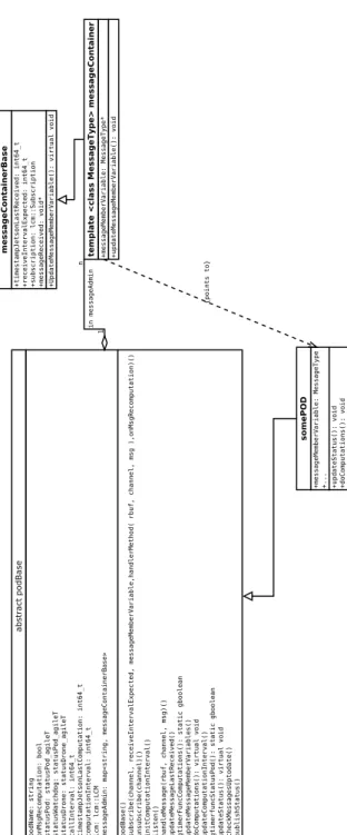
3-2 podBase-Class UML diagram . . . 42
3-3 Quadrotor Status: State Machine . . . 43
3-4 Remote Communication Diagram . . . 45
3-5 3D Viewer for Flight Telemetry . . . 46
4-1 Coordinate Frames . . . 48
5-1 Thresholded Image of View on Marker Setup . . . 58
5-2 Polygons found by RDP . . . 59
5-3 Identified Markers . . . 60
5-5 Fullstate EKF: Signal Flow . . . 67
5-6 Hybrid Fullstate Filter: Performance . . . 76
5-7 Fullstate EKF: Performance . . . 77
6-1 Cascaded Control Scheme . . . 83
6-2 Controller Synthesis Diagnostics . . . 92
6-3 Stochastic Optimal Controller on Simple Dynamics: 2D Trajectories . 95 6-4 Stochastic Optimal Controller on Simple Dynamics: Control and 3D trajectories . . . 95
6-5 Stochastic Optimal Controller under Challenging Initial Condition . . 96
6-6 Stochastic Optimal Controller on Full Dynamics: 2D Trajectories . . 97
6-7 Stochastic Optimal Controller on Full Dynamics: 3D Trajectories . . 98
6-8 Motorcommander Signal Flow . . . 99
7-1 Experimental Scene Setup . . . 102
7-2 Hover Flight Trajectories . . . 104
7-3 Target Region Flight with PD Control, 2D Trajectories . . . 106
7-4 Target Region Flight with PD Control, velocities . . . 107
7-5 Target Region Flight with PD Control, orientation and acceleration . 107 7-6 Target Region Flight with Stochastic Optimal Control, 2D Trajectories 109 7-7 Target Region Flight with Stochastic Optimal Control, velocities . . . 109
7-8 Target Region Flight with Stochastic Optimal Control, orientation and acceleration . . . 110
List of Tables
2.1 Quadrotor Hardware Parameters . . . 26
4.1 Aerodynamic Effects on Thrust . . . 52
5.1 Hybrid Filter: Noise covariances . . . 65
5.2 EKF: Noise Covariances . . . 74
A.1 Aerodynamic Parameters . . . 119
A.2 Marker Detection Parameters . . . 120
A.3 PD Controller Gains . . . 120
Chapter 1
Introduction
1.1 Motivation
Over the last few years quadrotors have become increasingly popular in industry, con-sumer entertainment, research and amongst hobbyists. Many open source projects offer solutions ranging from simple flight controllers up to the full suite of compo-nents that are required for versatile deployment of unmanned aerial vehicles (UAV) including control, guidance and mission planning [40]; engineering magazines fea-tured tutorial-style introductions to modeling, planning and control of quadrotors [42]; undergraduate controls classes have been taught using toy drones [36].
For researchers, the quadrotors’ high maneuverability, complex underactuated dy-namics and affordable price point make them an attractive platform choice to demon-strate novel approaches to robotic autonomy.
However, limited onboard computing power oftentimes creates severe bottlenecks. These bottlenecks lead to two types of quadrotors: a) completely autonomous but slow-moving vehicles with larger size, weight and power requirements as in [49]; b) fast, agile platforms that require a priorly known environment and offboard support through motion capture systems (as in [44]) or planning algorithms.
This separation impeded transitioning new solutions from the lab environment to real-world field deployment. Bridging this gap requires taking solution for estimation
and scene understanding used in slow, fully autonomous platforms to smaller plat-forms and speed them up under the constraint of limited onboard computing power. Control algorithms need to account for nonlinear effects that cannot be neglected dur-ing more agile maneuvers any longer [52]. Figure 1-1 illustrates this problem setup conceptually. On the one hand, a heavily researched solution approach falls under
Figure 1-1: Bridging the Gap between Agile and Autonomous Quadrotors: Via lightweight algorithms, or upgraded hardware.
the notion of ’lightweight algorithms’ where the low computational complexity shall enable them to be used onboard of small platforms as in [3] or [57]. On the other, recent developments in the realm of embedded computing promise to bridge the gap by significantly upgrading the computational hardware.
The main contribution of this thesis is the design and implementation of a small quadrotor platform equipped with a high-performance embedded computing unit that enables the use of high-rate, high-resolution computer vision for visual-inertial estima-tion, and the implementation of optimal control policies designed using compressed-continuous computation methods based on tensor-train-decomposition.
power with an additional integrated GPU unit. The quadrotor platform built in this thesis is developed from the ground up to accommodate this computing unit without additional overhead in mechanical design. The quadrotor’s sensor set allows complete vision-based autonomy. This work also comprises the development of a comprehensive set of software components including software in the loop simulation, safety handling and estimation and control algorithms. To maximize the usability of the platform for further research purposes, a motion capture system is fully integrated into the system. Testing validates the platform’s usability.
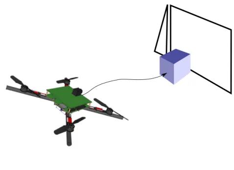
A use case scenario that guides this thesis compares most adequately to disaster relief scenarios where quadrotors are used to explore environments fast and autonomously, e.g. partly destroyed buildings. In this setup, quickly navigating through openings like doors, windows and holes is an important task.
Figure 1-2 gives an abstract visualization of this task: A scene target within a scene is identified and a target region for the quadrotor to fly to is derived from the location of this scene target. In this thesis, the scene target is a marker setup that resembles a window.
Plenty of research has been focused on relatively slow maneuvers such as hover and landing as e.g. presented in [61]. On the contrary, flying aggressive trajectories has required the use of fast motion capture systems ([44] or [8]). These systems guarantee high estimation accuracy. A controller’s robustness margin therefore needs to cover model inaccuracies only, but less so estimation inaccuracies. Aggressive maneuvers have therefore mostly been confined to lab spaces. We hypothesize that a potential solution with promising outlook is to provide a stochastic optimal controller solved to global optimality for initial conditions in the entire state space. With this controller, not being able to track an "optimal trajectory" does not imply leaving the trajectory’s region of attraction. In fact, there is no one precomputed trajectory but an optimal feedback control policy for every point in state space. However, solving for these optimal control policies under nonlinear systems generally suffers from the curse of dimensionality: The complexity scales exponentially with the number of dimensions
Figure 1-2: Scene Environment with quadrotor, marked window as scene target and target region to fly through (purple).
in the worst case [11]. Novel approaches in applying tensor-train-decomposition-based optimization to dynamic programming of stochastic optimal control problems are able to offer a solution. An optimal control policy for a 7-dimensional stochastic system was presented in [24]. This thesis demonstrates, as a proof-of-concept, the use of these new kind of controllers for quadrotor control under visual-inertial fullstate estimation.
1.2 Related Work
Over the last years research work on quadrotors and research utilizing quadrotor platforms have been increasing steadily. They are used to demonstrate vision-based estimation algorithms, trajectory planning, mapping and novel control algorithms. This section introduces work related to this thesis.
Hardware Multiple related open source projects exist. Some of them started aca-demically and are now spun off into companies: Gurdan et al. present a small, energy-efficient quadrotor with high-rate sensor data acquisition well suited for
re-search [26]. Now, companies like Ascending Technologies offer comparable platforms [4]. The Pixhawk project [43] designed an open-source low-latency, high-performance hardware/controller-suite that builds on top of the LCM-communication framework (LCM is also used in this thesis and discussed in detail in Section 3.2). The Ardupi-lot- and Dronecode-projects have grown to a large, industry-supported open source project to foster the deployment of "cheaper, better and more reliable unmanned aerial vehicles" [41]
Estimation Early work on quadrotors as well as experiments involving highly dy-namic flight maneuvers relied on external support for both computation and mation. Expensive motion capture systems provided accurate and fast position esti-mates ([44] or [8]). With increasing computing power on smaller and smaller devices, researchers started to shift computational load away from these external, offboard resources. Achtelik et al. present a lower cost alternative to motion capture sys-tems using illuminated colored balls mounted on the quadrotor that could be tracked from external cameras [2]. With the nascence of smaller and lighter cameras, novel platforms now oftentimes include vision-based estimation and navigation. The di-verse vision-assisted estimation and control concepts can be divided into groups of increasing capabilities to solve high-level tasks:
Image-based visual servoing addresses the task to make a quadrotor hover over or in front of given visual cues and operates on image-level measurements. Chaumette [13] and Hutchinson [33] give introductions to this topic. Approaches for image-based trajectory tracking, taking into account the underactuated dynamics of quadrotors are discussed by several authors [28],[27],[37]. Grabe et al. [25] use onboard computed optical flow to stabilize a quadrotor’s position.
Position-based visual servoing, in turn, addresses a comparable task but usually estimates the quadrotor’s full state, as e.g. presented in [61] for vision-based take-off, hovering and landing. This relates closely to full visual-inertial estimation that fuses vision-based measurements with accelerometer and gyroscopic data to generate fullstate estimates. Taking away priorly known visual cues from the environment
moves this estimation task into the realm of simultaneous localization and mapping (SLAM), where not only the robot’s pose is estimated, but also the position of fea-tures in the environment. An introduction and comprehensive survey is given by [10]. Many researchers exploit different variations of SLAM: some approaches do not include running a full SLAM to reduce computational load to enable onboard compu-tation ([52] or [1]) or to enable heuristic real-time obstacle avoidance [3]. This kind of onboard visual-inertial estimation proved to enable accurate figure flying [34].
3D-reconstruction of the environment and mapping applications like [20], [35] or [39] build on top of that. Barry et al. exploit the nonholonomic dynamics of UAVs and present a novel, computationally inexpensive algorithm for stereo matching [7]. These approaches enable steps towards improved scene understanding. More complex platforms include, e.g., laser scanners for better scene understanding during outdoor-indoor transition [49].
Planning and Control Much research has been conducted on designing fast and reliable control and trajectory planning algorithms. Since quadrotors are highly dy-namic systems, aggressive trajectories can be realized, but the planned trajectories need to comply with the platform’s dynamic constraints. Shen at el present a trajec-tory planning algorithm for quadrotors that takes into account the trajectrajec-tory’s effect on vision-based estimates [53]. Costante et al. propose a perception-aware path plan-ning approach to find trajectories that best support the vision-based state estimation [15]. An approach for real-time trajectory planning through given waypoints in flat output space under dynamic constraints is discussed in [45]. Quadrotors that are capable of juggling poles are presented by [8]. To increase the agility, a quadrotor with variable pitch has been designed by [16]; they are able to fly multiple flips.
A popular control approach, also summarized in the comprehensive tutorial [42], utilizes a cascaded control scheme where an outer-loop-controller generates a reference orientation from translational state errors. This reference orientation is then tracked by an orientation-inner-loop-controller. This approach is also detailed in 6.2 in this thesis. Nonlinear controllers have been designed to work directly on the nonlinear
dynamics and achieve convergence for flight states far away from hover conditions [42] [53].
Very recently, techniques for compressed computation have been applied to stochas-tic optimal control problems. Horowitz et al. solve an optimal control problem in high dimensions by exploiting linear HJB equations and give a simulated quadrotor example [30]. Gorodetsky et al. introduce a general framework to solve stochastic optimal control problems that does not require linear HJB equations and can han-dle input constraints [24]. This thesis utilizes this control framework to compute an optimal feedback controller that complies with the nonlinearity, actuator constraints and stochasticity of the quadrotor dynamics.
1.3 Contributions
The main contributions of this thesis can be divided into two aspects: (a) hardware implementation and software architecture design, including estimation and control solutions, and (b) a proof-of-concept demonstration in simulation and experiment of using stochastic optimal controllers, computed through tensor-train-decomposition-based compression techniques.
Specifically,
1. The designed quadrotor platform is equipped with a high-performance embed-ded computing unit with a GPU that enables the use of fast, high-resolution computer vision, estimation and control on board.
2. The provided baseline estimation is set up as visual-inertial estimation and runs fully on board. The developed platform offers sufficient computing reserves to add scene understanding, feature tracking or obstacle detection using standard approaches from e.g. the openCV libraries that can exploit the onboard GPU unit.
3. The modular software design allows to easily switch in and out new estimators, controllers, feature trackers, etc. Due to the use of the
LCM-message-handling-framework low data exchange latency is achieved and signals from high-level tasks down to motor-level commands can be handled by the same infrastruc-ture.
4. A tensor-train-decomposition-based approach is used to synthesize a globally optimal controller that complies with the nonlinear, stochastic quadrotor dy-namics and actuator constraints.
5. Simulation studies and experiments present a proof-of-concept for the usability of these recent developments in utilizing compressed computation techniques for controller synthesis.
1.4 Organization
This thesis is organized as follows:
Chapter 2 details the hardware and electronics design of the quadrotor platform. Design considerations and selection of components are discussed. Chapter 3 describes the software architecture and introduces the roles of various system components like estimators, controllers and vision-related software pieces. The setup reveals the ease of substituting in new or additional software parts. It also presents the communication architecture between quadrotor, motion capture system and ground station.
The mathematical models for the quadrotor’s dynamics are given in Chapter 4, including actuator and battery dynamics. A simulator features all these phenomena. Chapter 5 presents the visual detection of a scene target and two estimation algorithms to generate fullstate estimates. Both use priorly known visual features in the environment and onboard accelerometer and gyroscopic measurements. The estimators’ performance is evaluated with experimental data.
Chapter 6 describes a control structure that cascades the underactuated dynamics into a position- and an orientation subsystem. Two controllers are discussed for the position subsystem: first, a commonly used PD controller that acts on linearized
dynamics. Second, a globally optimal, stochastic optimal controller that takes into account the nonlinearity of the quadrotor dynamics and actuator constraints. In this chapter, the controller performance is evaluated in simulation.
An experimental performance evaluation of the overall integrated systems is pre-sented in Chapter 7. It shows the platform’s hover capabilities and demonstrates that tensor-decomposition-based nonlinear stochastic optimal controllers can control the quadrotor to approach a target region.
Finally, Chapter 8 summarizes this thesis, discusses limitations and suggests start-ing points for future work.
Chapter 2
Quadrotor Hardware Implementation
This chapter describes the quadrotor’s hardware design and the electronic architec-ture. The platform was built entirely from the ground up using a variety of off-the-shelf components from both hobbyist RC-stores and specialized manufacturers like PointGreyResearch. This approach allowed to build an optimized platform to ac-commodate the NVIDIA TK1 computing unit and the required sensor setup for full autonomy without additional mechanical overhead. The following sections cover the overall architecture, the computing unit, the sensor setup, the actuation system and the motion capture system which was used to acquire ground truth data.
In addition, for subsystems like the camera with static, geometric parameters, the identified parameters are discussed in this chapter.
2.1 System Architecture
This section introduces the quadrotor’s overall design and architecture.
The quadrotor carbon-fiber frame Turnigy Talon V2 is an off-the-shelf quadrotor frame and was chosen for its capability to house the TK1 computing unit in its center. Additional electronic components were installed on a PCB board above the TK1. Figure 2-1 shows the current version of the quadrotor platform. In this flight-ready configuration, with all components mounted including batteries, a safety cage and motion capture markers, the platform weighs 1.28kg. Its inertia values, determined
by a bifilar pendulum experiment, and propeller geometry data can be found in Table 2.1.
Figure 2-1: Quadrotor Build
Table 2.1: Quadrotor Hardware Parameters
mass 𝑚 1.28 kg inertia (𝐽𝑥𝑥, 𝐽𝑦𝑦, 𝐽𝑧𝑧) (6.9𝐸−3, 7.0𝐸−3, 12.4𝐸−3) Ns2 propeller diameter 𝑑𝑝 0.165 m propeller positions r𝐵 prop [︀±0.117 ±0.117 −0.012]︀ 𝑇 m
A standard Wifi module, Intel 7260, provides the Wifi connection to a ground station computer for real-time data visualization and user-input capabilities. No real-time-critical data is streamed between the ground station and the quadrotor.
On the sensor side, the flight scenario that is being considered for this thesis re-quires an IMU for high-bandwidth orientation estimation and a monocular camera for
lower-rate localization and position estimation. On the actuation side, four brushless motors were used to provide thrust with off-the-shelf propellers. For data-collection and safety purposes, it is possible to switch between autonomous flight mode and human-controlled flight mode. A separate microcontroller, an Arduino nano, gener-ates the PWM signals that command the motors. This setup enables the operator to use a switch on the RC controller to switch between motor commands generated by either the onboard computing unit or by the entirely self-contained, off-the-shelf quadrotor flight controller (AfroFlight Naze32 ).
To prevent bandwidth and interference complications in data transfer all components are connected through individual buses to the central TK1 computing unit. Figure 2-2 details the connections.
Figure 2-2: Electronics Diagram
2.2 Computation Unit
While there are many options to choose from for onboard-computing power, the NVIDIA TK1 computing unit poses a noticeable step-up in computational capabili-ties in comparison to often used microcontrollers. The TK1 features an ARM-Cortex A15 Quadcore CPU with 2.32 Ghz, 2Gb RAM, 16GB memory, an NVIDIA Kepler
GPU with 192 cores and various interfaces like HDMI, I2C, UART, USB 3.0 or Eth-ernet. It delivers up to 300 gflops. Its power consumption rarely exceeds 5W, but can go up to 15W under highly demanding tasks. These specifications allow for complex computations at high rates. The manufacturer showcases feature tracking at 720p at 40 fps. This thesis exploited this computational power to run high-resolution com-puter vision for pose estimation and real-time controller optimization at a sufficiently high rate to allow for agile maneuvering of the quadrotor. The TK1’s low weight of about 130g allowed to mount it onto the quadrotor, thus running all processes on board the platform.
The platforms’s power supply is split into two separate circuits as shown in Fig. 2-4: a 4S Lithium-Polymer-battery provides power to the computing unit as well as the USB-hub that powers the camera, the Naze32 flight controller and the Arduino; a 3S Lithium-Polymer-battery powers the motors. This setup minimizes electrical noise induced by power spikes from varying motor load.
Figure 2-3: NVIDIA’s Jetson TK1 [47]
2.3 Sensor Setup
This section discusses the details of the sensor setup. An IMU provides measure-ments for angular rates and acceleration and can therefore provide high-bandwidth information for position and orientation estimates. The camera is used for lower-rate updates of pose estimates with respect to an identified scene target.
Future versions of the platform will contain a battery voltage sensor and possibly measurements of motor speeds. Programmable ESCs like the VESC [58] could offer a handy solution to this (although the current version is too large).
2.3.1 Inertial Measurement Unit
The current configuration features a BOSCH BNO055 IMU on a Sparkfun break-outboard. The IMU-chip offers onboard filter capabilities. Using a custom-extended version of [50] the gyroscope’s and accelerometer’s bandwidth were set to 41Hz. The angular rates and acceleration are then read through a dedicated thread on the TK1 computing unit via an I2C-connection at 100Hz. It turned out that the propellers induce significant mechanical vibrations into the frame. With some IMUs this caused extremely noisy accelerometer readings and sometimes even a shift in accelerome-ter bias. The use of damping mounts to dampen out mechanical vibrations greatly improved the sensor data.
2.3.2 Camera
The platform’s camera, a Flea 3 FL3-U3-13Y3M-C from Point Grey Research (Fig-ure 2-5) offers up to 150 FPS at 1280x1024 pixels. While for p(Fig-ure navigation purposes a high-resolution high-rate camera, as chosen for this project, might not be necessary, it does improve the localization accuracy with respect to a visual scene target. Impor-tantly, it features a global shutter, simplifying the use of raw images for estimation purposes.
It is connected via USB 3.0 to a powered, dedicated USB-3.0 hub.
Figure 2-5: PointGreyResearch’s Flea 3 Camera [48]
[51] provides a model and toolbox to calibrate omni-directional and fish-eye cameras. It maps a 2D-image point pfish = [𝑢 𝑣]𝑇 to a 3D-unit-vector mcamemanating from the
camera system’s ’single effective viewpoint’. All real-world points lying on this ray result in the same pfish.
Assuming perfectly aligned lenses, [51] shows that
mcam= ⎡ ⎢ ⎢ ⎢ ⎣ 𝑋 𝑌 𝑍 ⎤ ⎥ ⎥ ⎥ ⎦ cam = ⎡ ⎢ ⎢ ⎢ ⎣ 𝑢 𝑣 𝑓 (𝑢, 𝑣) ⎤ ⎥ ⎥ ⎥ ⎦
With a perfectly symmetric lens, 𝑓(𝑢, 𝑣) can further be simplified to 𝑓(𝑢, 𝑣) = 𝑓(𝜌) with 𝜌 being the pixel-distance of a point pfish from the image center. The function
𝑓 (𝜌) is approximated by an n-th order polynomial. The toolbox suggests a default order of 4. In our experiments this choice of parameters yielded reasonable results. The calibration run for the lens used on the quadrotor resulted in parameters
𝛼0 = −5.518𝐸2 𝛼1 = 0 𝛼2 = 8.372𝐸−4 𝛼3 = −6.474789𝐸−7 𝛼4 = 1.236𝐸−9
following
2.4 Actuator Characteristics
The quadrotor’s four propellers are driven by Sunnysky 22107S brushless-DC-motors. They are commanded by ZTW Spider Opto electronic speed controllers (ESC). These ESCs are capable of handling up to 30A and are controlled using PWM-signals with a length between 1ms and 2ms at up to 400Hz update-rate. The power supply is separate from the supply to the computation and sensing architecture.
Standard 6” quadrotor propellers are installed.
2.4.1 Propellers
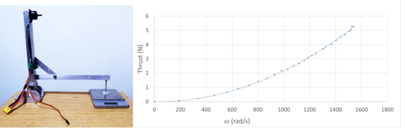
Using a custom-made rig pictured in Figure 2-6 the relation from propeller speed/motor speed to generated thrust was identified. Motor speeds were measured using a Ex-tech digital laser tachometer. While this identification does not account for in-flight aerodynamic effects caused by, e.g., relative wind velocities, it does not suffer from the influence of ground effects because the design features a horizontal propeller axis, resulting in horizontal air flow.
The ESCs were commanded through the same software framework that was used to later fly the quadrotor in autonomous mode.
The recorded data follows a quadratic relation, thus complying with the classic
(a) Rig for Static Thrust Estima-tion 0 1 2 3 4 5 6 0 200 400 600 800 1000 1200 1400 1600 1800 Th ru st (N ) w (rad/s)
(b) Data Points Static Thrust
model for propeller thrust:
𝑇 = 𝛼𝑇𝜔2
with 𝑇 being the thrust generated and 𝜔 being the motor speed in rad/s. The identification resulted in
𝛼𝑇 = 2.26𝐸−6
2.4.2 Speedcontrollers and Battery
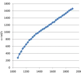
The software flight controllers output desired motor speeds which need to be converted into PWM-signals with pulse length 𝜅 microseconds that can be sent to the ESCs. An identification of the relation between 𝜅 and motor speed is therefore necessary. This relation is, however, heavily influenced by a decreasing battery charge state since the terminal voltage drops not only with load (which is covered by the identification procedure), but also over time with an increasingly depleted battery. The ESCs do not compensate for this effect.
To mitigate this effect, the identification is conducted with a fully charged battery, quick enough to not noticeably deplete the battery. ESCs are oftentimes tuned to reproduce a near linear relation between generated thrust and 𝜅 (in steady-state). Since 𝑇 ∝ 𝜔2, an approximate relation √𝜔 ∝ 𝜅 could be expected. Indeed, the
resulting identification revealed a clear square-root relation for lower motor speeds, and a rather linear relation for high speeds (Figure 2-7).
This procedure neglects the fact that three additional motors will draw current from the same battery during flight, especially during high motor speeds - further reducing the battery’s terminal voltage, which, in turn, additionally reduces the thrust and renders the identification less accurate. Section 4.2.3 sets up a parametrized model
0 200 400 600 800 1000 1200 1400 1600 1800 1000 1200 1400 1600 1800 2000 w ra d/ s k
Figure 2-7: Data Points PWM 𝜅 to Motor Speed 𝜔: Near-square root-relation
to account for this effect and presents the identified values.
2.4.3 Motors
Neglecting electrical time scales, electric motors generally follow approximate, first-order delay dynamics. Figure 2-8 shows a short-time-Fourier-transformed (STFT) audio recording of an ESC-controlled motor being ramped up from below-hover to take-off motor speed. It reveals that this first-order delay dynamics persist with an ESC in the loop. 4.2.4 elaborates on the modeling of this effect.
Figure 2-8: Short-Time-Fourier-Analysis of Motor Sound on Stepinput: Plot reveals first-order delay dynamics.
2.5 Motion Capture System
A motion capture system provided position estimates for initial flight experiments and ground truth to evaluate onboard position estimates. This system was newly set up for these experiments. The OptiTrak-System [46] features 6 infrared Flex 13W cameras, capable of providing full 6D-pose estimates of rigid-bodies at up to 360Hz. Infrared-reflective markers are mounted onto the drone in an asymmetric way to provide unambiguous identification to the OptiTrak pose-estimation-algorithm. Fishing nets were used to build a safety cage around the flying area. Figure 2-9 shows the setup of the motion capture area.
3m 3.5 m
5.5m
7m 6.5m
Chapter 3
Software Implementation
This chapter discusses the software architecture. Since the onboard computing unit is capable of running of full Linux system (Linux4Tegra L4T), the software design was inspired by architectures that have previously been designed to run on stan-dard desktop computers. All code was written in C++ and the PODs-framework [5] was used as software development guideline. In the remainder, threads - or dedi-cated processes - are called PODs themselves. These resemble nodes from the known RobotOpertingSystem ROS.
3.1 Multithread Architecture
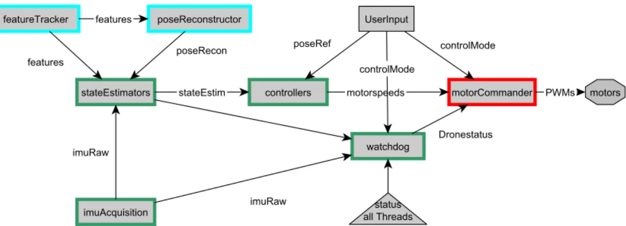
Full autonomy requires various computational tasks to be completed simultaneously: Sensor data is acquired, filtered, combined and augmented through estimators; con-trollers decide on the desired action to be executed by actuators. These different processes have been distributed into separate PODs. They exchange data by passing messages. Again, this design closely resembles a ROS-design. The message passing system, however, is implemented using LCM. Section 3.2 gives a brief description. Figure 3-1 illustrates the resulting network of PODs and the required messages being passed between them. The PODs are run at three different update rates: Visual feature detection runs at 50Hz, IMU data acquisition, estimation, control and safety checks (watchdog-POD) at 100Hz and the motorCommander at 200Hz.
Figure 3-1: Multithread Architecture with Messages and Update rates: cyan (50Hz), green(100Hz), red(200Hz).
The featureTracker detects the scene target and publishes calibrated 3D rays em-anating from the camera to the features. The detection algorithm is detailed in Section 5.1.1.
The poseReconstrutor reconstructs the full 6D-pose, consisting of orientation and po-sition. It uses a standard openCV-pnp-algorithm and is discussed in more detail in 5.1.2.
The stateEstimators take IMU-raw data, visual features and potentially the visually reconstructed pose to estimate the full 12-dimensional state of the quadrotor. Details can be found in Chapter 5.
The controllers convert the current state estimate into desired motor speeds. Chapter 6 elaborates on the design of various controllers.
The watchdog runs safety checks to shut down the quadrotor in case of emergencies or software faults. Figure 3-3 illustrates the safety checks with a state machine. The motorCommander selects which controller’s desired motor speeds are being con-verted into PWM-values that are then sent out to the Arduino nano that generates the PWM-signals to command the motors via the ESCs.
3.2 Thread Communication using LCM
The communication between different PODs is handled by the Lightweight Commu-nications and Marshalling framework (LCM) [32]. The LCM-libraries were developed by MIT’s DARPA Urban Challenge team to provide a high-bandwidth, low latency tool for message passing with bindings to various programming languages. Similarly to ROS, PODs can publish messages to and receive from user-specified channels using the LCM-libraries. This thesis chose LCM over ROS to avoid computational overhead and minimize latency in message handling.
3.3 Design of Base Thread
Every POD thread instantiates a worker object from a class that is derived from a POD-base-class podBase. These worker objects store data needed for the computa-tions they do. For example, the full-pose position controller thread controllerPDPose instantiates a controllerPDPose-object derived from the podBase-class. This section describes how the base class podBase offers functionality to do computations and re-ceive and publish messages in a multithreaded way.
Figure 3-2 shows its UML diagram. The member variables:
∙ podName represents the name of the POD. It is used to publish a status message about its "health" on a channel "statuspodName".
∙ onMsgRecompuation is a flag to enable rerunning the POD’s computation-method on receiving any new message.
∙ statusPOD stores the POD’s status.
∙ statusWatchdog represents the POD’s local copy of the watchdog’s current sta-tus. The podBase-class constructor autosubscribes every POD to the message channel that contains the watchdog-POD’s status; i.e., every POD knows about the watchdog’s status.
∙ same for statusDrone.
∙ callInterval: the interval which the POD’s computation loop is called at by a gLib-loop.
∙ timestampJetsonLastComputation: a timestamp when the most recent compu-tation loop was completed.
∙ computationInterval: the duration of the most recent computation.
∙ lcm: the lcm-object. This member object offers LCM-functionalities like sub-scribing or actively listening to an LCM channel.
∙ messageAdmin: A map that stores information about all the messages that the POD is subscribed to. It maps from the channel name to a messageContainer object which is derived from a virtual base class messageContainerBase. This allows to iterate through the map, thus iterating through all messages that the POD is subscribed to and e.g. executing operations on all messages.
The member methods:
∙ subscribe: subscribes the POD to a channel. The POD will use receiveInterval-Expected to check whether it is up-to-date on messages from this channel. A new messageContainer with key "channel" is added to the messageAdmin. This function also calls the actual LCM-subscribe-function and passes the handler-method that is called upon receiving a new LCM-message. This handler handler-method is per default the handleMessage-function.
∙ unsubscribe unsubscribes the POD from an LCM-message-channel by removing the corresponding item from the messageAdmin-map and by calling the LCM object’s unsubscribe-function.
∙ initComputationInterval initializes variables related to checking the execution time of the computation method.
∙ listen is a simple while loop that calls LCM’s handle function which makes it listen for new messages coming in over the LCM network. LCM’s handle() waits until it gets a new message and then calls the function handle handler-Method which was passed on subscribing an LCM object to a channel. The listen function is run in a separate, dedicated thread. This requires taking care of multithreaded variable access.
∙ handleMessage is the default handler method that is being called by the LCM object on receiving a new message. It blocks the access to the messageAdmin and stores the new message in the corresponding messageContainer in the mes-sageAdmin. It also updates the meta information about receive intervals stored in the messageContainers by calling updateMessageLastReceived. In case on-MsgRecomputation is enabled (in general or for this specific channel) and the POD’s computation loop is currently not running, it runs the computation loop.
∙ gtimerFuncComputation is the static method whose handle is fed into a gLib-timer function. On being called it first copies all messages stored in the mes-sageAdmin to the POD’s corresponding member variables by calling updateMes-sageMemberVariables. UpdateMessageMemberVariables uses the messageAdmin to iterate through all messages that the POD is subscribed to and make them update their corresponding POD’s member variables. Then, the POD’s specific doComputation-function is run, executing the actual computations. After be-ing done it updates the computation interval the computation took. With this setup, the doComputation-method can simply use the worker object’s mem-ber variables to access the most recent LCM messages that the POD received. Mutex-locking the access to the messageAdmin and the member variables only occurs during the copy and update-process. This setup handles the fact that the listener-method runs in a different thread simultaneously and has write-access to the messages stored in the messageContainers.
∙ gtimerFuncStatusPod is the static function fed into a second gLib-loop. It calls the POD’s specific updateStatus-function after copying the most recent
messages from the messageAdmin to the local member variables by calling up-dateMesageMemberVariables. updateStatus checks if messages are up-to-date by calling checkMessageUptodate and implements POD-specific health checks before it publishes the POD’s status by calling publishStatus.
On the messageContainerBase-class:
This abstract class provides a base class that holds meta information about a sub-scribed channel and the most recent message received from that channel.
∙ timestampJetsonReceived stores when a new message was received last from this channel.
∙ receiveIntervalExpected stores the interval which new messages from this channel are expected to arrive at
∙ subscription holds the pointer to the lcm-subscription that corresponds to the message. This objects can be used to e.g. unsubscribe.
∙ messageReceived is typeless pointer to the most recently received message.
∙ updateMessageMemberVariable() is a virtual method that is implemented in a child class and calls the child’s updateMesageMemberVariable(). This function copies the message in messageReceived into the corresponding member variable of the POD object while mutex-locking the access.
A templated class derived from messageContainerBase is then used to instantiate messageContainers that "know" about the actual type of the message (instead of merely having typeless void pointers to stored messages) and that contain a mes-sageMemberVariable pointer that points to the POD’s member variable that receives a copy of the most recently received corresponding message and can be used to do computations with.
3.4 System Status and Safety Handling
Since the overall system has multiple subsystems, each with different initialization procedures, a system status variable is introduced. This droneStatus is being used to handle both the initialization status and the emergency status. The emergency sta-tus aspect of this implementation can be considered the software-sided safety hand-ing, in addition to the experimental setup (the net cage) and the electronic safety switch using a separate Arduino to switch between human-RC-controlled mode and autonomous mode.
Figure 3-3 illustrates the state machine with transition conditions and motorCom-mander (the POD that communicates with the ESCs through the Arduino) action taken in each state. The state machine runs in the watchdog-POD.
te mp lat e <c la s s Mes sage T yp e> me ss a g eCont ainer + me ss ag eM em be rV ar ia bl e : Me ss ag eT yp e* + up da te Me ss ag eM em be rV a ri ab le () : vo id abs tract podBa se + po dN am e: s tr in g + on Ms gR ec om pu ta ti on : b oo l + st at us Po d: s ta tu sP od _ ag il eT + st at us Wa tc hd og : st at u sP od _a gi le T + st at us Dr on e: s ta tu sD r on e_ ag il eT + ca ll In te rv al : in t6 4_ t + ti me st am pJ et so nL as tC o mp ut at io n: i nt 64 _t + co mp ut at io nI nt er va l: in t6 4_ t + lc m: l cm :: LC M + me ss ag eA dm in : ma p< st r in g, m es sa ge Co nt ai ne r Ba se > + +po dB as e( ) + su bs cr ib e( ch an ne l, r e ce iv eI nt er va lE xp ec te d , me ss ag eM em be rV ar ia b le ,h an dl er Me th od ( rb u f, c ha nn el , ms g ), o nM sg Re co mp ut at io n) () + un su bs cr ib e( ch an ne l) ( ) + in it Co mp ut at io nI nt er v al () + li st en () + ha nd le Me ss ag e( rb uf , c ha nn el , ms g) () + up da te Me ss ag eL as tR ec e iv ed () + gt im er Fu nc Co mp ut at io n s( ): s ta ti c gb oo le an + up da te Me ss ag eM em be rV a ri ab le s( ) + do Co mp ut at io ns () : vi r tu al v oi d + up da te Co mp ut at io nI nt e rv al () + gt im er fu nc St at us Po d( ) : st at ic g bo ol ea n + up da te St at us () : vi rt u al v oi d + ch ec kM es sa ge sU pt od at e () + pu bl is hS ta tu s( ) i n me ss ag eA dm in 1 n me s sage Co nta ine rBa s e + ti me st am pJ et so nL as tR e ce iv ed : in t6 4_ t + re ce iv eI nt er va lE xp ec t ed : in t6 4_ t + su bs cr ip ti on : lc m: :S u bs cr ip ti on + me ss ag eR ec ei ve d: v oi d * + Up da te Me ss ag eM em be rV a ri ab le () : vi rt ua l vo i d s o m eP OD + me ss ag eM em be rV ar ia bl e : Me ss ag eT yp e + .. . + up da te St at us () : vo id + do Co mp ut at io ns () : vo i d { po in ts t o}
3.5 Remote Communication
This section addresses the remaining need for remote communication for a quadrotor that does not require offboard computation or processing.
The quadrotor sends all its flight telemetry data through an LCM tunnel using a standard Wifi module to a central router.
To acquire ground truth data, a motion capture system was installed. Its software runs on a separate Windows computer and sends pose estimates (position, orientation and translational velocities computed with filtered finite differences) as UDP multicast packages over a Gigabit Ethernet to the central router. Note that the quadrotor can receive these packages. It timestamps them and converts them into LCM messages.
A groundstation desktop computer was used to receive all flight telemetry data through an Ethernet LCM tunnel for visualization purposes. Additionally, user-input for different flight-modes or target position can be streamed to the quadrotor.
To manually fly the drone for data-recording and safety purposes the quadrotor features the AfroFlight Naze32, an off-the-shelf flight controller. This flight controller receives a desired quadrotor orientation from an FrSky Taranis Plus RC-flight con-troller over radio signal.
Based on one channel of the radio signal, the Arduino switches between creating the PWM-signal from PWM-values received from the TK1 computing unit or received from the Naze32 Flight Controller. This switch-channel is linked to a button on the RC control.
Figure 3-4 illustrates this communication architecture.
3.6 Simulation and Visualization Environment
For efficient testing and tuning of control parameters, a simulation environment was setup in MATLAB/Simulink. [36] was extended to model additional phenomena (discussed in Chapter 4). [36] is an extended version of Peter Corke’s toolbox [14].
auto-code-Figure 3-4: Remote Communication Diagram
generation and interfaced with a POD. This POD feeds the simulation with motor speed inputs and publishes simulation outputs like the full, simulated quadrotor state, sensor readings and visual features. The full software framework including estimation and control PODs can therefore simply be run "simulator in the loop".
LCM provides real-time viewers to display data published over the LCM network. For analysis purposes, this data can be converted into MATLAB format using a tool provided by the libbot-library [31]. A libbot-based viewer-POD subscribes to relevant quadrotor telemetry and visualizes the actual and estimated quadrotor states together with thrust in 3D in real-time (Figure 3-5). Note that the channels subscribed to to acquire the visualization data can either be generated from a simultaneous simulation, or from recorded, real in-flight data.
Figure 3-5: 3D Viewer for Flight Telemetry: Simulated state (green), and EKF-estimated state (purple; with offset for better visibility).
Summary
This chapter described the software architecture and introduced the roles of various system components like estimators, controllers and vision-related software pieces. The setup revealed the ease of substituting in new or additional software parts. It also presented the communication architecture between quadrotor, motion capture system and ground station.
The next chapter presents the mathematical models for the quadrotor’s dynamics including actuator and battery dynamics.
Chapter 4
System Dynamics Modeling
This section introduces the mathematical models used to describe the quadrotor’s dynamics. While these models can be arbitrarily complex to account for various effects, the following two models were chosen: The simplest model that still fully describes all six degrees of freedom of a quadrotor. This model will be used to derive controllers. The model used for simulation takes into account additional phenomena like battery effects, motor dynamics and simple aerodynamics.
4.1 Quadrotor Model
4.1.1 Coordinate Frames
Figure 4-1 shows the major coordinate systems used in the derivations of the dynamic equations:
Let r𝐼 be the position of the quadrotor’s center of mass in an inertial global
coordinate frame
r𝐼 = [︁
𝑥𝐼 𝑦𝐼 𝑧𝐼 ]︁𝑇
ex-𝑥𝐵 𝑧𝐵 𝑦𝐵 𝑥𝐼 𝑦𝐼 𝑧𝐼 r𝐼 𝑟 𝑞 𝑝 m𝐼,1
Figure 4-1: Coordinate Frames with Marked Window and Target Region
pressed in the global frame
v𝐼 = ˙r𝐼 =[︁˙𝑥𝐼 𝑦˙𝐼 ˙𝑧𝐼]︁𝑇
The origin of a body-frame coordinate system {𝑥𝐵, 𝑦𝐵, 𝑧𝐵}is fixed to the quadrotor’s
center of mass and the axes line up with the principal axes as illustrated. The quadrotor’s orientation 𝜂 is expressed in euler-angles (yaw, pitch, roll)
𝜂 =[︁𝜓 𝜃 𝜑 ]︁𝑇
relating to a rotation first about the global Z axis (yaw 𝜓), then a pitch-rotation 𝜃 about the new y-axis, followed by a roll-rotation 𝜑 about the new x-axis.
The matrix W−1 transforms the body-angular rates
Ω = (𝑝, 𝑞, 𝑟)𝑇
about local x-y-z-axes to euler-rates
˙
𝜂 =[︁𝜓˙ 𝜃˙ 𝜑˙ ]︁𝑇
Let T𝐵 be the total thrust generated by the rotors expressed in the body frame.
Let 𝜏𝑦𝑎𝑤 be the total torque about the (body-frame) 𝑧𝐵-axis resulting from propeller
drag. Motor speed acceleration is neglected. Let 𝜏𝑝𝑖𝑡𝑐ℎand 𝜏𝑟𝑜𝑙𝑙 be the resulting torque
about 𝑦𝐵-axis and 𝑥𝐵-axis, respectively. Let J be the quadrotor’s inertia expressed
in the body frame.
4.1.2 Basic Quadrotor Model
This section now introduces the simplest dynamic model to describe the quadrotor’s dynamics with its full 6-DOF.
Let the state x be composed of global position r𝐼, orientation 𝜂, global velocities v𝐼
and body-frame angular rates Ω:
x = [︁r𝐼 v𝐼 𝜂 Ω ]︁𝑇
Derived from from a standard Newtonian approach with total thrust T𝐵 acting on
the center of mass, and body-frame torques 𝜏𝑖 as the plant inputs, the quadrotor
dynamics result in (as derived in e.g. [21], with neglected gyroscopic effects)
˙r𝐼 = v𝐼 ˙ vI = G𝐼+ D𝐼𝐵(𝜂)T 𝐵 𝑚 ˙ 𝜂 = W−1Ω J ˙Ω = ⎡ ⎢ ⎢ ⎢ ⎣ 𝜏𝑟𝑜𝑙𝑙 𝜏𝑝𝑖𝑡𝑐ℎ 𝜏𝑦𝑎𝑤 ⎤ ⎥ ⎥ ⎥ ⎦ − Ω × JΩ with D𝐼
𝐵 denoting the rotation matrix from body-frame axes to the inertial frame
axes, either as function of euler-angles 𝜂
where D𝜓 = ⎡ ⎣ cos(𝜓) − sin(𝜓) 0 − sin(𝜓) cos(𝜓) 0 0 0 1 ⎤ ⎦ D𝜃 = ⎡ ⎣ cos(𝜃) 0 cos(𝜃) 0 1 0 − sin(𝜃) 0 cos(𝜃) ⎤ ⎦ D𝜑 = ⎡ ⎣ 1 0 0 0 cos(𝜑) − sin(𝜑) 0 sin(𝜑) cos(𝜑) ⎤ ⎦
or as function of a quaternion q that represents the same orientation:
D𝐼𝐵(q) = ⎡ ⎢ ⎢ ⎢ ⎣ 𝑞20+ 𝑞21 − 𝑞2 2 − 𝑞23 2(𝑞1𝑞2 − 𝑞3𝑞0) 2(𝑞1𝑞3+ 𝑞2𝑞0) 2(𝑞1𝑞2+ 𝑞3𝑞0) 𝑞02− 𝑞21+ 𝑞22− 𝑞32 2(𝑞2𝑞3− 𝑞1𝑞0) 2(𝑞1𝑞3− 𝑞2𝑞0) 2(𝑞2𝑞3+ 𝑞1𝑞0) 𝑞20− 𝑞12− 𝑞22+ 𝑞23 ⎤ ⎥ ⎥ ⎥ ⎦
The quaternion representation follows
q = ⎡ ⎣ 𝑞 e ⎤ ⎦= ⎡ ⎢ ⎢ ⎢ ⎣ 𝑞0 ... 𝑞3 ⎤ ⎥ ⎥ ⎥ ⎦
where 𝑞 = 𝑞0 represents the scalar and e the complex part of the orientation
quater-nion. Note that ||q|| = 1. Furthermore, W−1 = ⎡ ⎢ ⎢ ⎢ ⎣
0 sin(𝜑)cos(𝜃) cos(𝜑)cos(𝜃)
0 cos(𝜑) − sin(𝜑) 1 sin(𝜑) tan(𝜃) cos(𝜑) tan(𝜃)
⎤ ⎥ ⎥ ⎥ ⎦
It is to be noticed that this system is underactuated since it has six degrees of freedom but only 4 actual control inputs (the four motors speeds 𝜔𝑖. The conversion from
motor speeds 𝜔𝑖 to
[︁
T𝐵 𝜏roll 𝜏pitch 𝜏yaw
]︁𝑇
is detailed in 4.2.2). However, due to coupling effects, any position r𝐼 and yaw-angle 𝜓 can be achieved as steady-state.
Differentially flat models use exactly these four coordinates [r𝐼 𝜓] as output space
[45].
4.2 Actuator Models
The model introduced above uses physical torques 𝜏𝑖 and total thrust T𝐵 as plant
in-puts. However, these inputs result from motor speeds which are themselves subject to additional dynamics (motor-, battery and ESC-dynamics). Additionally, the introduc-tory quadrotor tutorial [42] points out and summarizes relevant aerodynamic effects that affect the generation of thrust T𝐵,𝑖 on each propeller. This section describes
these phenomena. The simulation environment introduced in Section 3.6 features all these effects.
4.2.1 Aerodynamic Effects
Mahoney et al. [42] provide an overview of quadrotor estimation and control topics, including a brief introduction to the effects of blade flapping and induced drag. These effects are considered to have significant influence on the dynamics, especially since they generate forces occurring in the body-frame x-y-plane - which is under-actuated since the propeller thrust - the only force-control input (without these effects) - is fully aligned with the body-frame z-axis.
When the quadrotor moves in its x-y-plane, the advancing propeller blade has a higher absolute tip velocity than the retreating blade. This causes the propeller blades to bend. Due to the high rotor velocity, gyroscopic effects occur and induce a torque perpendicular to the apparent wind direction. Consequently, the thrust is not aligned with the motor axes any longer and points backwards with respect to the velocity direction of the quadrotor. Induced drag also results from different relative airspeeds of advancing vs retreating propeller blades: Since the advancing blade moves faster, it produces more lift, but also more drag than the retreating blade. The net effect is an additional, the "induced", drag. [42] also demonstrates how both effects can be modeled in a lumped model. Peter Corke’s toolbox [14] models these effects. (Note that this toolbox is part of the simulator set up for this thesis (cf. Section 3.6)).
4.2.2 Motor Speed-Thrust Conversion
This section describes how [14] modeled the conversion from the four motor speeds to the plant input [︁T𝐵 𝜏
roll 𝜏pitch 𝜏yaw
]︁𝑇
used in the system model above.
The total thrust T𝐵 results from the sum of four propeller thrusts T𝐵,𝑖, where the
thrust vectors’ directions are determined by above mentioned aerodynamic effects:
T𝐵 = 3 ∑︁ 𝑖=0 T𝐵,𝑖 where T𝐵,𝑖 = 𝑇𝑖 ⎡ ⎢ ⎢ ⎢ ⎣
− cos(𝛽aero,𝑖) sin(𝛼aero,𝑖) sin(𝛽aero,𝑖)
− cos(𝛼aero,𝑖) cos(𝛽aero,𝑖) ⎤ ⎥ ⎥ ⎥ ⎦ 𝐵
with 𝛽aero,𝑖 and 𝛼aero,𝑖 being detailed in Table 4.1; additional parameters can be found
in the Appendix in Table A.1.
Table 4.1: Aerodynamic Effects on Thrust as in [14]
Relative air speed at propeller 𝑖: v𝐵
ra,𝑖 Ω × r𝐵prop,𝑖+ D𝐵𝐼(𝜂)v𝐼 Planar components: 𝜇𝑖 √︁ 𝑣𝐵 x,ra,𝑖2+ 𝑣y,ra,𝑖𝐵 2 /|𝜔𝑖𝑑2𝑝|
Non-dimensionalized normal inflow: 𝑙𝑖 𝑣𝐵z,ra,𝑖 2
/|𝜔𝑖𝑑2𝑝|
Sideslip azimuth relative to x-axis: 𝑗𝑖 atan2(𝑣y,ra,𝑖𝐵 , 𝑣𝐵x,ra,𝑖
Sideslip rotation matrix: Jss,𝑖 [︂cos(𝑗sin(𝑗𝑖) − sin(𝑗𝑖) 𝑖) cos(𝑗𝑖) ]︂ Longitudinal flapping: 𝛽lf,𝑖 J𝑇ss,𝑖 [︂((8 3𝜃b0+ 2𝜃b1) − 2𝑙𝑖/(1/𝜇𝑖− 𝜇𝑖/2) 0 ]︂ 𝛼aero,𝑖 𝛽𝑥,lf,𝑖− 16𝑞/(𝛾aero|𝜔𝑖|) 𝛽aero,𝑖 𝛽𝑦,lf,𝑖− 16𝑝/(𝛾aero|𝜔𝑖|)
For the body-frame torques 𝜏 = [𝜏𝜑 𝜏𝜃 𝜏𝜓] it is 𝜏 = 3 ∑︁ 𝑖=0 r𝐵prop,𝑖× T𝐵 𝑖 + 𝑄𝑖 ⎡ ⎢ ⎢ ⎢ ⎣ 0 0 1 ⎤ ⎥ ⎥ ⎥ ⎦ with r𝐵
prop,𝑖 being propeller 𝑖’s position with respect to the quadrotor’s center of mass
and 𝑄𝑖 = 𝛼𝑄𝜔𝑖|𝜔𝑖|being the propeller-drag-induced torque.
Most basic models neglect these aerodynamic effects and assume 𝛼aero = 𝛽aero = 0,
thus assuming the thrust vectors to be fully aligned with the body-frame z-axis. This results in T𝐵 𝑖 = [0 0 𝑇𝑖]𝑇 and T𝐵 = [︁ 0 0 𝑇 ]︁𝑇
where 𝑇 = ∑︀ 𝑇𝑖. Under these assumptions, the plant input reduces from the six
dimensional [︁T𝐵 𝜏 𝜑 𝜏𝜃 𝜏𝜓 ]︁𝑇 to a four dimensional u =[︁𝑇 𝜏𝜑 𝜏𝜃 𝜏𝜓 ]︁𝑇 . With 𝑇𝑖 = 𝛼𝑇𝜔𝑖2 from 2.4.1, above equations can be reformulated as
u = ⎡ ⎢ ⎢ ⎢ ⎢ ⎢ ⎢ ⎣ 𝑇 𝜏𝜑 𝜏𝜃 𝜏𝜓 ⎤ ⎥ ⎥ ⎥ ⎥ ⎥ ⎥ ⎦ = MuT ⎡ ⎢ ⎢ ⎢ ⎢ ⎢ ⎢ ⎣ 𝜔20 𝜔2 1 𝜔22 𝜔2 3 ⎤ ⎥ ⎥ ⎥ ⎥ ⎥ ⎥ ⎦ = 𝛼𝑇 ⎡ ⎢ ⎢ ⎢ ⎢ ⎢ ⎢ ⎣ 1 1 1 1
𝑟y,0 𝑟y,1 𝑟y,2 𝑟y,3 𝑟x,0 𝑟x,1 𝑟x,2 𝑟x,3 𝛼𝑄 𝛼𝑇 − 𝛼𝑄 𝛼𝑇 𝛼𝑄 𝛼𝑇 − 𝛼𝑄 𝛼𝑇 ⎤ ⎥ ⎥ ⎥ ⎥ ⎥ ⎥ ⎦ ⎡ ⎢ ⎢ ⎢ ⎢ ⎢ ⎢ ⎣ 𝜔02 𝜔2 1 𝜔22 𝜔2 3 ⎤ ⎥ ⎥ ⎥ ⎥ ⎥ ⎥ ⎦
This gives an invertible relation between squared motor speeds 𝜔𝑖 and the plant input
u = [𝑇 𝜏𝜑 𝜏𝜃 𝜏𝜓]𝑇. This allows to design controllers on the basic quadrotor model with
input u and, during flight, translate a given desired actuator action u*(𝑡)into desired
motor speeds 𝜔*(𝑡) to command the motors. Parameters for this equation can be
4.2.3 Speed Controller-Battery Model
The hardware section 2.4.2 on battery and ESC characteristics mentioned the fact that changing terminal voltage changes the steady-state motor speeds even when PWM-signals that are being sent to the ESC remain constant. While a dropping terminal voltage as a result of a depleting battery state was not modeled, a simplified parametrized battery model was used to account for the effect of the terminal volt-age dropping with increased current that is drawn from the battery. The following assumptions are made: the battery follows a Thevenin Equivalent Circuit with con-stant voltage source and an internal resistance; this results in the terminal voltage dropping proportionally to current drawn; the current drawn is proportional to the torque required from the motors to overcome rotational propeller drag; this torque is proportional to the thrust produced; thrust is proportional to the squared motor speeds; under ideal battery conditions, the ESC achieves a linear relationship between PWM value 𝜅𝑖 and the squared motor speeds; squared motor speeds therefore drop
linearly with dropping terminal voltage.
A simple, approximate model derived under these assumptions is
𝜅𝑖 = 𝛼ESC𝜔*2𝑖 𝑈0− ∑︀ motors𝑗(𝛼Bat𝜔 * 𝑗)2 + 𝜅0
A nonlinear least-squares resulted in estimated parameters:
𝛼ESC = 0.0033 𝑈0 = 11.5
𝛼Bat = 6.5310−4 𝜅0 = 1074
Note that this equation can be inverted when taking into account all four 𝜔*
𝑖 and 𝜅𝑖:
The simulator used to simulate the quadrotor’s dynamics takes the commanded 𝜅𝑖
and outputs the corresponding steady-state 𝜔*
𝑖.
ad-dresses the noticeable transient in achieving this steady-state.
4.2.4 Motor Model
The hardware description in Section 2.4.3 pointed out that the closed-loop system of motor and ESC - with the PWM-value 𝜅 being the input signal and actual motor speed 𝜔 the output signal - roughly follows first-order delay dynamics when feeding a step-input.
From the STFT plot in Figure 2-8, the time constant is approximated as
𝑡𝑚 = 0.06
for both upwards and downwards steps, resulting in a transfer function from a desired motor speed 𝜔* (corresponding to some PWM value 𝜅) to an actual motor speed 𝜔:
𝜔(𝑠) = 1 𝑡𝑀𝑠 + 1
𝜔*(𝑠)
Summary
This chapter presented the mathematical models for the quadrotor’s dynamics in-cluding actuator and battery dynamics.
The following chapter introduces the visual detection of a scene target and two estimation algorithms to generate fullstate estimates that comply with the dynamical models presented in this chapter. The estimators’ performance is evaluated with experimental data.
Chapter 5
Visual-inertial State Estimation
This chapter discusses vision-based scene target detection and two approaches to synthesize a fullstate estimate with respect to that scene target. An experimental evaluation of the estimation performance is presented. Unlike e.g. image-based visual-servoing, the controller solution in this thesis separate the estimation and control problem. Therefore, a fullstate estimate is required. Recalling that a possible scenario for a quadrotor of this design could be to explore buildings in disaster relief scenarios, entering through openings like doors and windows becomes a crucial task. While a vision-based window detection is not the focus of this thesis, a detection is still needed to present a full proof-of-concept. For this purpose, the visual detection problem was simplified as much as possible.
5.1 Vision-based Localization
In this section, two algorithms are described: first, a simple approach to reliably find a scene target at high-rates. A marked window forms this scene target. Second, the known pnp-pose reconstruction algorithm (where pnp stands for perspective-n-Point) that is commonly used to reconstruct a camera pose from identified image features with known 3D real-world locations.
5.1.1 Scene Target Detection
Since the detection problem is not focus of this thesis, the experimental setup was designed such that the real-world markers (oftentimes referred to as landmarks) and their corresponding image features are most easily detectable and unambiguously identifiable at high rates.
In the chosen experimental setup, a window-like structure was imitated by a dark rectangle and triangle on a white wall (Figure 5-1). It is positioned at the back end of the flying area, around 𝑥𝐼 = 3.0𝑚. This structure enabled a reliably
unam-biguous identification of all corners on an image level - independent from any other estimates - and therefore proved to be a convincing choice as image features. The global 3D-positions of these corners have been measured using the motion capture system. AprilTags or colored dots were considered as an alternative. However, the first approach showed robust results at rates above 50Hz.
The algorithm to find and identify the seven corners of the marker setup is described in the following paragraphs. First, the gray-scale image is thresholded, resulting in an image shown in Figure 5-1. This thresholded image is then fed into openCV’s
findContours-function. A Ramer-Douglas-Peucker-algorithm (RDP) [29] is applied to fit polygons to the contours, effectively reducing the number of points of each contour. The approximation tolerance is chosen such that the marker triangle and rectangle are robustly approximated as three and four-point polygons for a wide range of camera poses. The resulting image with fitted polygons is shown in Figure 5-2. The set of all three- and four-point polygons is then searched for a pair with
Figure 5-2: Polygons found by RDP
a ratio 𝜁 = |pfish,T𝑖 −p fish,R
𝑗 |min
|pfish,T𝑖 −pfish,R𝑗 |max with 𝜁 < 𝜁 < ¯𝜁 (where p fish,T
𝑖 ,pfish,R𝑗 denote the pixel
locations in the original image of the triangle and rectangle corners, respectively), and 𝐴 < 𝐴rectangle
𝐴triangle < ¯𝐴, with 𝐴 denoting the area of the polygons. Parameters can be
found in Table A.2.
This approach proved to be robust enough to uniquely and unambiguously identify the 7 corners of the triangle and rectangle. Figure 5-3 shows an overlay of original image and identified markers.