HAL Id: hal-02303653
https://hal.archives-ouvertes.fr/hal-02303653
Preprint submitted on 2 Oct 2019
HAL is a multi-disciplinary open access
archive for the deposit and dissemination of
sci-entific research documents, whether they are
pub-lished or not. The documents may come from
teaching and research institutions in France or
abroad, or from public or private research centers.
L’archive ouverte pluridisciplinaire HAL, est
destinée au dépôt et à la diffusion de documents
scientifiques de niveau recherche, publiés ou non,
émanant des établissements d’enseignement et de
recherche français ou étrangers, des laboratoires
publics ou privés.
To cite this version:
B Fedele, C. Negulescu, M. Ottaviani. Asymptotic-preserving method for the vorticity equation. 2019.
�hal-02303653�
Asymptotic-preserving method for the
vorticity equation
B. Fedele
1, C. Negulescu
1and M. Ottaviani
2†
1Institut de Math´ematiques de Toulouse, Universit´e Paul-Sabatier, Toulouse, France.
2CEA, IRFM, F-13108 Saint-Paul-lez-Durance, France.
(Received xx; revised xx; accepted xx)
We present an Asymptotic-Preserving method to solve numerically the two-dimensional vorticity-Poisson (Navier-Stokes) system. The main focus is the validation of the numer-ical scheme. As test cases we consider the unforced evolution of Taylor-Green vortices and the forced Kolmogorov flow with a sinusoidal source term. The scheme is validated by comparing the results with those obtained with an explicit spectral code and with an analytic result about the linear instability regime. We show that the AP-properties of the method allow one to deal efficiently with the multi-scale nature of the problem by tuning the time step to the physics one aims to study and not by stability constraints. As a side result, we investigate the long time scale evolution of the Kolmogorov flow, observing that it evolves into a final stable stationary state characterised by a seemingly universal relation between stream-function and vorticity.
1. Motivation, background and objectives
The scope of this paper is to present an efficient numerical method to deal with a class of problems coming from incompressible fluid mechanics, of which the paradigm is the two-dimensional vorticity equation:
(V)ϵ ⎧ ⎨ ⎩ ∂tωϵ+ 1 ϵu ϵ · ∇ωϵ= (∆ ωϵ − ∆ ωeq) , (t, x)∈ R+× Ω , −∆Ψϵ= ωϵ, uϵ=⊥∇Ψϵ, (t, x)∈ R+× Ω , (1.1) where x := (x, y) ∈ Ω with Ω an open, bounded domain of R2, in our case a rectangle. The problem is complemented by periodic boundary conditions and it consists of an evolution equation for the vorticity ωϵ, coupled to the Poisson equation for the computation of the stream-function Ψϵ. This latter function is fixed by imposing the constraint⟨Ψϵ
⟩ = 0 where ⟨·⟩ denotes the average over the domain Ω . The perpendicular gradient operator is defined as ⊥∇ := (∂
y,−∂x) . The parameter ϵ∈ (0, 1) models the stiffness of the problem, and its physical significance will be explained in Section 1.1. The term ωeqappearing on the right hand side of system (1.1) denotes a forcing term. In this paper, we examine two well-known vortex-problems: the Taylor-Green flow (unforced case ωeq(x) = 0) and the Kolmogorov flow (forced case ωeq(x) = cos(x)), with special emphasis on the stability properties of these flows. The study of such simple flows is precious, as it helps to acquire intuition and insight by displaying the particular behavior of the flow under the influence of different physical mechanisms and also by providing ideal test cases for checking numerical methods. Our main focus will be the numerical investigation of the instability of equilibria-flows described by (1.1), and this via an Asymptotic-Preserving scheme (Klar 1998; Jin 1999). In particular, we are interested
in the validation of the proposed AP-scheme, which was especially designed to capture efficiently and accurately all ϵ-regimes, notably the ϵ→ 0 limit regime.
In this work we restrict the study to 2D flows. This is done primarily for practical reasons, while developing and validating the scheme. There is however a practical interest about flows occurring in Nature that exhibit 2D dynamics, such as those found in geophysical, astrophysical and oceanographic context. These flows are subject to strong geometrical constraints, so that the vertical motion can be often neglected (hurricanes, the Great Red Spot of Jupiter, the vortex Gulf Stream, etc.). We refer the interested reader to Lugt (1983) for a review of vortex dynamics in Nature. In the context of magnetised plasma physics, such quasi-2D flows can occur as a consequence of the strong magnetic field which induces a strongly anisotropic dynamics. The earliest model equation was derived by Hasegawa & Mima (1977). It describes the evolution of the electric potential in a plane perpendicular to the magnetic field and it is only slightly more general than the model studied in the present work.
The Taylor-Green flow is a particular 2D vortex flow, which evolves from a single-Fourier mode initial condition (for ex. ωin= 2 sin x sin y), without forcing (ωeq(x) = 0). The analytic solution is known in this case and will be considered as the time-dependent equilibrium-solution to be perturbed. Without perturbation the initial vortices are damped in time by dissipation, while keeping the same shape. It is however well-known, that this solution is unstable, giving rise, when perturbed, to mixing processes or filamentation, leading eventually to a state with a completely reconfigured final flow. The Taylor-Green flow can be considered as a model of the Von Karman flow such as the one depicted in figure 1, panel (a).
The Kolmogorov flow corresponds to a 2D, one-directional shear flow, with sinusoidal velocity profile, which is maintained by a forcing term (ωeq(x) = cos(x)), in the presence of viscosity. It admits a stationary solution, the laminar Kolmogorov flow, which can be unstable under certain conditions. One then observes the emergence of complex time-dependent structures, leading first to a characteristic island pattern (also sometimes called cat’s eye), then, as the systems evolves, to a complete rearrangement of the flow, leading to a stationary end state. The Kolmogorov flow can be considered as a paradigm of a channel flow without boundaries such as the one sketched in figure 1, panel (b). Studying the instability of shear flows is a notorious numerically difficult problem. Indeed, the occurrence of several time and space scales (eddies with a wide range of sizes), as well as the sensitivity of the solution (unstable equilibria) to numerical errors, make numerical integration delicate. In particular, if one is interested in capturing long-time asymptotics, efficient numerical schemes are needed, allowing one to control the accumulation of the errors over the time. Simulation methods that do not pay sufficient attention to these issues are likely to fail. Numerical strategies must take full advantage of the asymptotic properties of the underlying problem in order to be efficient. In view of all these difficulties, our present aim is to introduce and validate an Asymptotic-Preserving method, which allows one to overcome the above mentioned complications. In particular, such a scheme should be able to reach directly the equilibrium state (when it exists), skipping the intermediate states, and as a consequence, avoiding the error accumulation. Moreover, by exploiting the asymptotics of the problem at hand, the scheme can largely reduce the computational time when one is interested in the large time scale dynamics. In the rest of this work, we rewrite the system (V)ϵas :
AP method for the vorticity equation 3
(a) Von Karman flow.
viscous friction, linear (bottom) friction, and lateral walls (confinement), which are characterized by the three dimen- sionless parameters Y, ,u, and N. Adopting the concept of confinement to the present stability problem, we distinguish between the elementary system, which is a flow consisting of one spatial period (N = 19 of the Kolmogorov flow and be- ing bounded by walls at y = 0 and y = 27r, extended systems, where confining walls are located at y = 0 and y = 27rN (N> l), and the unbounded system extending from y = - CO toy = + CO. Results of the stability of the elemen- tary and extended systems are reported in Sec. III, whereas Sec. IV is devoted to the treatment of the unbounded system. We calculate the precise critical values of parameters at which instability sets in and we discuss the structure of the first unstable modes. Finally, in Sec. V, we relate our results to experimental findings in electromagnetically driven flows and explain the connection between the full magnetohydro- dynamic equations and the dimensionless equation, which serves as a basis for our theoretical studies.
Figure 1 shows the sequence of instabilities observed by Kolesnikov’“~l’ in a series of experiments where one spatial period of a Kolmogorov flow in a straight duct serves as the basic state [Fig. 1 (a) I. The liquid metal flow is driven by a homogeneous magnetic field interacting with an electric cur- rent injected through the bottom of the duct by line elec- trodes. At a fixed value of the magnetic field, the strength of the electric current lis a measure of the Lorentz force driv- ing the flow and represents, thereby, the control parameter. Above a threshold I,, a traveling wave with fixed wave num- ber is observed [Fig. 1 (b) 1. For larger 1, when more wave numbers are linearly unstable, the system exhibits processes of wave-number interaction [Fig. 1 (c) I. Finally, intermit- tent turbulent spots lead to fully developed turbulence [Fig. l(d)]. In the experiments of Bondarenko et al.’ the basic flow comprises three periods of the Kolmogorov flow
(a) (b) (cl id) --. h -- r -
FIG. 1. Instability in an elementary period of the Kolmogorov flow ob- served by Kolesnikov:‘“~” (a) basic laminar flow, (b) traveling wave slightly above instability threshold, (c) wave-number interaction, and (d) turbulence.
1386 Phys. Fluids A, Vol. 4, No. 7, July 1992
ues of the electric current, the stationary secondary flow pat- tern undergoes a Hopf bifurcation resulting in an oscillatory state. For very high 1, chaotic oscillations of the flow pat- terns were observed. In recent experiments, Batchaev” in- vestigated in detail the dependence of the longitudinal wave numbers at instability onset on the number of periods for systems between N = 2 and 11. This wave number appeared to be fairly sensitive to N as long as N is small and almost independent of the transverse confinement ifNis sufficiently high. Fully turbulent regimes in extended systems (N> 19
have not yet been observed in experiments. The theoretical investigation of Kolmogorov flow started with the work of Meshalkin and Sinai’ in which a large-scale instability at Re, = 42 was found for the purely viscous case. Bondarenko et al5 demonstrated that this threshold is shifted to much higher values if a linear bottom friction term is included into the theoretical model (see also, Obukhovi3 and Gledser et a1.14). Important progress was made by Beaumont I5 and Gotoh et a1.r6 by including into the consideration such modes that do not have the same periodicity in they direc- tion as the basic flow. They first applied Floquet theory to the Kolmogorov flow, thereby laying the foundation for a systematic treatment of the stability of spatially periodic flows with respect to quasiperiodic perturbations. A com- plete formalism for spatially and temporally periodic flows applicable to arbitrary space dimension is given in the recent work of Frenkei.r7 In this paper, the notion of guasinormal modes is introduced in order to distinguish the quasiperiodic structure of the unstable modes from the purely periodic normal modes of stability problems possessing continuous translational symmetry. We shall adopt this formulation in the formulation of the stability problems that follow. A dif- ferent approach to the stability of spatially periodic flows is used by Dubrulle and Frisch” based on the assumption of scale separation between the basic flow and unstable modes. A multiple scale analysis provides an explicit (formal) expression for the eddy viscosity tensor of parity invariant periodic flows. In contrast to the unbounded flows, only one theoretical treatment is known of a wall-bounded flow, namely that of Ponomarjov,” who found an increased criti- cal Reynolds number in the elementary purely viscous sys- tem.
Although nonlinear problems are beyond the scope of this paper, we mention the works ofKlazkin,” Green,” Si- vashinsksy,‘” and SheZ3 devoted to the construction of sim- plified models describing the nonlinear evolution of the Kol- mogorov flow above the instability threshold. A very detailed fully numerical simulation of the purely viscous Kolmogorov flow was performed by She.‘4
II. MATHEMATICAL FORMULATION OFTHE STABILITY
PROBLEM
Consider the two-dimensional flow of an incompressible viscous fluid which is governed by the dimensionless equa- tion
Andre Thess 1386
Downloaded 17 Jul 2006 to 171.66.38.133. Redistribution subject to AIP license or copyright, see http://pof.aip.org/pof/copyright.jsp
(b) Channel flow.
Figure 1: Two examples of flow, representing respectively the Von Karman flow (a) and a channel flow (b). (V)ϵ ⎧ ⎨ ⎩ ∂tωϵ+1 ϵ{ω ϵ, Ψϵ } = (∆ ωϵ − ∆ ωeq), (t, x)∈ R+× Ω , −∆Ψϵ= ωϵ, (t, x) ∈ R+ × Ω , (1.2) where{ωϵ, Ψϵ
} = ∂xωϵ∂yΨϵ−∂yωϵ∂xΨϵdenotes the Poisson bracket. This form is more adequate for simulations, as we will discretise the Poisson bracket with the Arakawa scheme (Arakawa 1966), which was devised specifically for such an advection term.
The outline of this paper is the following. In the remaining of Section 1, the phys-ical origin of system (1.1) is briefly reviewed, its multiscale nature is highlighted and some useful quantities are introduced. Section 2 deals with the Asymptotic-Preserving reformulation of our original problem (1.1) in order to obtain a more regular problem. This reformulation is based on a Micro-Macro decomposition of the unknown variable, and it is completed by a regularization procedure. The second part of Section 2 presents the numerical scheme that we develop in this paper. Section 3 focuses on the numerical study of the Taylor-Green test case. The main purpose of this Section is to validate our numerical procedure. Section 4 is dedicated to the study of the Kolmogorov flow. An analytic result about the relation between the growth rate of the linear instability of this flow and the aspect ratio of the domain is given. Furthermore, the nonlinear instability phase as well as the final state of the Kolmogorov flow are investigated. In particular, we find a functional relation between the stream function and the vorticity in the final state the numerical solution obtained by our numerical procedure. This article ends with Section 5 where some conclusions and perspectives are given.
1.1. Non-dimensional Vorticity-Poisson system
Our study is based on the incompressible Navier-Stokes equations, which describes a bi-dimensional flow with velocity u := (ux, uy, 0)T, pressure p and forcing term ueq:
(N S) $ ∂ tu + (u· ∇) u = −∇p + ν (∆ u − ∆ ueq) , (t, x)∈ R+× Ω , ∇ · u = 0 , (t, x) ∈ R+ × Ω , (1.3) Page 3 of 32
where ν denotes the kinematic viscosity of the fluid. The divergence-free constraint of u leads to the existence of a scalar stream-function Ψ such that u =⊥ ∇Ψ = (∂yΨ,−∂xΨ, 0)T. Introducing the vorticity ω = (∇ × u) · ez, we take the curl of (1.3) and then the scalar product with ez:= (0, 0, 1)T, to rewrite this system in the equivalent vorticity/stream-function form (V) $ ∂ tω +{ω, Ψ} = ν (∆ ω − ∆ ωeq), (t, x)∈ R+× Ω , −∆Ψ = ω , (t, x) ∈ R+ × Ω . (1.4)
In this work, we will consider different time scales. It is therefore useful to proceed with non-dimensional equations to identify the regimes of interest. For each function generically denoted by n(·) , we set n(·) := ¯n n′(·) , where ¯n refers to the characteristic scale of n(·) and n′ the non-dimensional associated function. With these notations, we now fix the spatial and time characteristic lengths ¯x and ¯t of the flow. Starting from the pair (¯x, ¯t), we deduce the characteristic scales of the other quantities:
¯ u = x¯¯ t , ω =¯ ¯ u ¯ x, Ψ = ¯¯ x ¯u .
Replacing in the vorticity problem (1.4) each quantity n(·) by ¯n n′, we obtain
(V) ⎧ ⎨ ⎩ ∂t′ω′+{ω′, Ψ′} = ν ¯t ¯ x2(∆ ω ′− ∆ ω′ eq), (t′, x)∈ R+× Ω , −∆Ψ′= ω′, (t′, x)∈ R+ × Ω . (1.5)
Introducing now a viscous time scale τν := ¯ x2
ν , the previous system can be written (V) ⎧ ⎨ ⎩ ∂t′ω′+{ω′, Ψ′} = ¯ t τν (∆ ω′− ∆ ωeq′ ), (t′, x)∈ R+× Ω , −∆Ψ′ = ω′, (t′, x)∈ R+ × Ω . (1.6) Supposing that the viscous time scale τν is very long compared to the observation time scale ¯t, we introduce the stiffness parameter ϵ standing for this ratio:
ϵ := t¯
τν ∈ (0, 1) .
If we are now interested in describing phenomena arising on non-viscous time scales, the vorticity model can be written as
(V)
$ ∂
t′ω +{ω, Ψ} = ϵ (∆ ω − ∆ ωeq) , t′ ∈ (0, T ) ,
−∆Ψ = ω , (1.7)
withT ∈ R+a fixed final time. On the other hand, if we are interested in characterizing phenomena arising on the viscous time scale, we set t = ϵ t′, and the Vorticity-Poisson system can be written as
(V)ϵ ⎧ ⎨ ⎩ ∂tωϵ+ 1 ϵ{ω ϵ, Ψϵ } = (∆ ωϵ− ∆ ωeq) , t∈ (0, T ) , −∆Ψϵ= ωϵ. (1.8) with T linked toT by the relation T = ϵ T . This is the starting point of our investigations.
1.2. Some quantities of interest
We recall here the definition of some integral quantities that will be used in our study. In the following,|Ω| denotes the measure of the domain Ω .
The kinetic energyKϵ(t, ωϵ), enstrophy
Eϵ(t, ωϵ) and palinstrophy Pϵ(t, ωϵ) are defined respectively by Kϵ(t, ωϵ) = 1 2|Ω| % Ω Ψϵ(t, x, y) ωϵ(t, x, y) dx dy = 1 2|Ω| % Ω|u ϵ(t, x, y) |2dx dy . Eϵ(t, ωϵ) = 1 2|Ω| % Ω [ωϵ(t, x, y)]2dx dy , Pϵ(t, ωϵ) = 1 2|Ω| % Ω [∇ ωϵ(t, x, y)]2dx dy . The time evolution of the kinetic energy is given by the relation
d dtK ϵ(t, ω) = −2 (Eϵ(t, ω) + Iϵ(t, u)) , where Iϵ(t, uϵ) = 1 2|Ω| % Ω
∆ ueq·uϵdx dy denotes the input energy through the external forcing velocity ueq.
The time evolution of the enstrophy satisfies d dtE ϵ(t, ωϵ) = −2 (Pϵ(t, ωϵ) + Jϵ(t, ωϵ)) , where Jϵ(t, ωϵ) = 1 2|Ω| % Ω
∆ ωeqωϵdx dy describes the enstrophy production through the external forcing ωeq.
We observe that the kinetic energy and the enstrophy decrease in time when the forcing term is zero.
We also introduce two quantities, the Rayleigh quotientRϵ(t, ωϵ) , and the dissipation quotient Λϵ(t, ωϵ): Rϵ(t, ωϵ) = E ϵ(t, ωϵ) Kϵ(t, ωϵ), Λ ϵ(t, ωϵ) =Pϵ(t, ωϵ) Eϵ(t, ωϵ).
The time derivative of the Rayleigh quotient verifies the following relation, obtained after simple computations d dtR ϵ(t, ωϵ) = −2 Rϵ(t, ωϵ) [Λϵ(t, ωϵ)− Rϵ(t, ωϵ) +Kϵ(t, ωϵ) (Jϵ(t, ωϵ)/Rϵ(t, ωϵ) −Iϵ(t, uϵ))] .
2. Numerical scheme
In this section we describe the numerical scheme we have developed for an efficient resolution of (1.1). We start by carrying out an Asymptotic-Preserving reformulation of the model. We then make use of the Arakawa scheme for the advection operators as well as the Diagonal Implicit Runge-Kutta (DIRK) approach for the time derivative.
Pϵ,h Pϵ P0,h P0 ϵ → 0 h→ 0 h→ 0 ϵ → 0
Figure 2: Commutative properties of AP-schemes.
2.1. Asymptotic-Preserving reformulation
An Asymptotic-Preserving scheme is a numerical approach designed to solve efficiently singularly-perturbed problems, denoted generically Pϵ, which contain some small param-eter ϵ ∈ [0, 1] . A precise definition of an AP-scheme is given in the next definition (see also commutative diagram in figure 2).
Definition 1. Consider a singularly-perturbed problem Pϵ, whose solution is assumed to converge (in a certain sense) towards the solution of a limit problem P0. An AP-scheme for Pϵ, denoted Pϵ,h, is a numerical scheme which enjoys the following properties:
• The AP-scheme Pϵ,h is stable in a suitable sense, uniformly in ϵ.
• For fixed stiffness parameter ϵ > 0 , the AP-scheme Pϵ,h provides a consistent discretization of the problem Pϵ, as h
→ 0 .
• For fixed discretization parameters h > 0 , the AP-scheme Pϵ,h provides in the limit ϵ→ 0 a consistent discretization of the limit problem P0.
Physical problems arising in nature are complex and contain several time and space scales, which are difficult to capture in their globality with standard schemes. Classical numerical procedures such as explicit methods are submitted to a CFL-condition, which forces the user to solve also the small scales of the problem, which can be sometimes undesirable. This leads necessarily to huge computational costs. Fully implicit methods can sometimes suffer from accuracy problems when the perturbation parameter is too small, as they do not capture the asymptotic limit. In such multi-scale frameworks, AP-schemes become interesting, as they allow eliminating those scales which are not relevant in the considered study without loosing accuracy and without stability problems. This aspect will be illustrated in the last part of this work.
The AP-reformulation we shall introduce for the resolution of (1.8) is based on the following decomposition of the vorticity field ωϵ into a macroscopic and a microscopic part, namely
ωϵ= χϵ+ ϵ ξϵ, (2.1)
where χϵ denotes the macroscopic part, which belongs to the kernel of the dominant transport operator TΨϵ :={ · , Ψϵ} and ξϵ denotes the microscopic part.
Inserting now (2.1) in (1.8), allows one to obtain the following system for the unknowns (ωϵ, ξϵ, Ψϵ):
(MM)ϵ ⎧ ⎪ ⎪ ⎪ ⎨ ⎪ ⎪ ⎪ ⎩ ∂tωϵ+{ξϵ, Ψϵ} = (∆ ωϵ− ∆ ωeq) , (t, x)∈ (0, T ) × Ω , {ωϵ, Ψϵ} − ϵ{ξϵ, Ψϵ} = 0 , (t, x) ∈ (0, T ) × Ω , −∆Ψϵ= ωϵ, (t, x) ∈ (0, T ) × Ω . (2.2)
This reformulation of (1.8) is now a regular problem in ϵ , allowing one to capture for ϵ→ 0 the limit problem (MM)0. Nevertheless, it is ill-posed since ξϵis not unique. To overcome this new problem, we shall employ a regularization technique already proposed in (Fedele et al. 2019), by inserting the term σ ξϵ in the second equation of (2.2) . We obtain then the final reformulated system:
(MM)ϵσ ⎧ ⎪ ⎪ ⎪ ⎨ ⎪ ⎪ ⎪ ⎩ ∂tωϵ,σ+{ξϵ,σ, Ψϵ,σ} = (∆ ωϵ,σ− ∆ ωeq) , (t, x)∈ (0, T ) × Ω , {ωϵ,σ, Ψϵ,σ } − ϵ{ξϵ,σ, Ψϵ,σ } + σ ξϵ,σ = 0 , (t, x) ∈ (0, T ) × Ω , −∆Ψϵ,σ = ωϵ,σ, (t, x) ∈ (0, T ) × Ω . (2.3)
Note that due to the regularization, (MM)ϵ
σ is no more equivalent to (MM)ϵ, however σ shall be chosen small enough, of the order of the truncation error, in order not to modify too much the initial problem.
2.2. Numerical discretization
We hereby describe in detail the numerical discretization of the reformulated system (2.3) .
2.2.1. Discretisation parameters
In what follows, we consider a bounded simulation domain ΩS:= (0, Lx)× (0, Ly) and all considered functions are supposed to be doubly periodic in x and y . The time interval [0, T ] , T > 0 , is discretized as follows :
tn:= n ∆t , ∆t := T /Nt, n∈ [[0, Nt]] , Nt∈ N .
In order to provide a uniform mesh on the domain ΩS, we define the grid spacings as follow :
xi:= (i− 1) ∆x , yj := (j− 1) ∆y , ∆x := Lx/Nx, ∆y := Ly/Ny,
where i∈ [[1, Nx+ 1]] , and j ∈ [[1, Ny+ 1]] . For any function f : [0, T ]× ΩS → R , fi,jn refers to the numerical approximation of f (tn, x
i, yj) , and fhn shall denote the discrete grid-function (fn
i,j)i,j. Because of periodic boundary conditions, we set :
fNnx+1,j= f n 1,j, fi,Nn y+1= f n i,1, ∀(n, i, j) ∈ [[0, Nt]] × [[1, Nx+ 1]]× [[1, Ny+ 1]] . 2.2.2. Space semi-discretisation
Let us proceed with the discretisation of the operators appearing in (2.3) . For the discrete Laplace operator evaluated at the point (xi, yj), one has
[∆hfh]i,j:= 1
∆x2(fi+1,j− 2 fi,j+ fi−1,j) +
1
∆y2(fi,j+1− 2 fi,j+ fi,j−1) .
(Arakawa 1966). For two functions f, g : ΩS → R, the discrete version of the Poisson bracket{f, g} evaluated at the point (xi, yj) is expressed by :
[fh, gh]i,j:= 1 12∆x∆y
'
fi+1,jAi,j+ fi−1,jBi,j+ fi,j+1Ci,j+ fi,j−1Di,j
+fi+1,j+1Ei,j+ fi−1,j−1Fi,j+ fi−1,j+1Gi,j+ fi+1,j−1Hi,j
( . where the coefficients write
Ai,j:= gi,j+1− gi,j−1+ gi+1,j+1− gi+1,j−1, Ei,j:= gi,j+1− gi+1,j,
Bi,j:= gi,j−1− gi,j+1− gi−1,j+1+ gi−1,j−1, Fi,j:= gi,j−1− gi−1,j,
Ci,j:= gi−1,j− gi+1,j− gi+1,j+1+ gi−1,j+1, Gi,j:= gi−1,j− gi,j+1,
Di,j := gi+1,j− gi−1,j+ gi+1,j−1− gi−1,j−1, Hi,j:= gi+1,j− gi,j−1.
We finish this paragraph with the discretisation of the Poisson equation−∆f = g . In order to limit the computational cost of the scheme, we resolve this latter by the Fourier method. For a discrete grid-function (fi,j)i,j, we denote by ()fp,q)p,q its discrete Fourier transform, where p∈ [[−Nx/2, Nx/2]] and q∈ [[−Ny/2, Ny/2]] . Introducing the quantities
kp = 2 π p Lx , kq = 2 π q Ly ,
the Poisson equation −∆f = g becomes, after the application of the discrete Fourier transform, ) fp,q = g)p,q k2 p+ kq2 .
And denoting by *f the inverse discrete Fourier transform of f , we obtain (fi,j)i,j = !()fp,q)p,q.
2.2.3. Time discretisation
In order to achieve second-order accuracy in time for the problem (2.3), we use a Diagonally Implicit Runge Kutta (DIRK) approach. The Runge-Kutta (RK) method is recalled here for clarity reasons (Alexander 1977).
We consider a problem of the form ∂tf = L(f ) + g(t) , where L denotes some differential operator and g a source term. An r-stage Runge-Kutta approach is characterized by its Butcher table
c1 a11 . . . a1r .. . ... ... cr ar1 . . . arr b1 . . . br .
For a given un, the subsequent un+1is defined by the formula
un+1= un+ ∆t r + j=1
bj(L(uj) + g(t + cj∆t)) ,
where each ui is defined by
ui= un+ ∆t r + j=1
ai,j(L(uj) + g(t + cj∆t)) .
Note that in the case where bj = arj for j = 1, ..., r , then un+1 is equal to the last stage of the method, namely ur. For our problem (2.3), we consider the following 2-stage Butcher table
µ µ 0
1 1− µ µ
1− µ µ .
In all our simulations, we choose µ := 1−1/√2 . With this choice, the method is L−stable (see Hairer & Wanner 1996, Sec. IV-3).
2.2.4. Fixed point procedure and final scheme
Due to the nonlinearity of our problem (2.3), in particular the fact that the function Ψϵ,σ is linked to the function ωϵ,σ via the Poisson equation, we have to develop a fixed point procedure in order to resolve numerically the problem (2.3) with an implicit numerical method. If we choose l ∈ N as an iteration index, the stream-function Ψϵ,σ can be considered as fixed during the iteration step l→ l + 1, given by the previous iteration. We denote by ∆t⋆the product µ ∆t .
For each time step n ∈ N, we are looking thus for (ωhϵ,σ,n+1, ξ ϵ,σ,n+1 h ), by iterating in l∈ N as follows. Starting from ωi,jϵ,σ,n+1,0:= ω ϵ,σ,n i,j , we have
⎧ ⎪ ⎪ ⎪ ⎪ ⎪ ⎪ ⎪ ⎪ ⎪ ⎪ ⎪ ⎪ ⎪ ⎪ ⎪ ⎪ ⎪ ⎪ ⎪ ⎪ ⎪ ⎪ ⎪ ⎪ ⎪ ⎪ ⎪ ⎪ ⎪ ⎪ ⎪ ⎪ ⎪ ⎪ ⎨ ⎪ ⎪ ⎪ ⎪ ⎪ ⎪ ⎪ ⎪ ⎪ ⎪ ⎪ ⎪ ⎪ ⎪ ⎪ ⎪ ⎪ ⎪ ⎪ ⎪ ⎪ ⎪ ⎪ ⎪ ⎪ ⎪ ⎪ ⎪ ⎪ ⎪ ⎪ ⎪ ⎪ ⎪ ⎩ Poisson solver: " Ψp,qϵ,σ,n+1,l= " ωϵ,σ,n+1,lp,q k2 p+ k2q . Stage 1: ωϵ,σ,n+1,l+11,i,j + ∆t⋆[ξϵ,σ,n+1,l+1 1,h , Ψ ϵ,σ,n+1,l h ]i,j= ωi,jϵ,σ,n+ ∆t⋆ ,-∆ωϵ,σ,n+1,l+11,h .i,j −-∆ωeq,h.i,j/, [ωϵ,σ,n+1,l+11,h , Ψ ϵ,σ,n+1,l h ]i,j− ϵ[ξϵ,σ,n+1,l+11,h , Ψ ϵ,σ,n+1,l h ]i,j+ σ ξ1,i,jϵ,σ,n+1,l+1= 0 . Stage 2:
ωϵ,σ,n+1,l+12,i,j + ∆t⋆[ξϵ,σ,n+1,l+12,h , Ψhϵ,σ,n+1,l]i,j= ωi,jϵ,σ,n+
1− µ µ (ω ϵ,σ,n+1,l+1 1,i,j − ω ϵ,σ,n i,j ) +∆t⋆,-∆ωϵ,σ,n+1,l+1 2,h . i,j− -∆ωeq,h.i,j/, [ωϵ,σ,n+1,l+12,h , Ψhϵ,σ,n+1,l]i,j− ϵ[ξϵ,σ,n+1,l+12,h , Ψ ϵ,σ,n+1,l h ]i,j+ σ ξ2,i,jϵ,σ,n+1,l+1= 0 . Final stage:
(ωϵ,σ,n+1,l+1i,j , ξi,jϵ,σ,n+1,l+1) = (ωϵ,σ,n+1,l+12,i,j , ξ2,i,jϵ,σ,n+1,l+1) .
(2.4) In all of the subsequent simulations, the stopping criterion chosen for these iterations (at l = lf) is 0 0 0||ωhϵ,σ,n+1,l+1||L1 h− ||ω ϵ,σ,n+1,l h ||L1 h 0 0 0 ||ωϵ,σ,n+1,lh ||L1 h + 0 0 0||Ψhϵ,σ,n+1,l+1||L1 h− ||Ψ ϵ,σ,n+1,l h ||L1 h 0 0 0 ||Ψhϵ,σ,n+1,l||L1 h < 10−2, where ||fh||L1 h := ∆x ∆y N+x+1 i=1 Ny+1 + j=1
|fi,j| denotes the discrete L1− norm of a grid function fh. We end the procedure by setting
ωi,jϵ,σ,n+1:= ωϵ,σ,n+1,lf+1
i,j ,
ξi,jϵ,σ,n+1:= ξ
ϵ,σ,n+1,lf+1
i,j .
Finally, the new stream-function at iteration n + 1 is computed then via
(Ψi,jϵ,σ,n+1)i,j = ! ( "Ψp,qϵ,σ,n+1)p,q, with Ψ"p,qϵ,σ,n+1:= " ωp,qϵ,σ,n+1 k2 p+ k2q .
We refer to the scheme developed in this section as (DAMM)-scheme for Dirk-Arakawa-Micro-Macro (scheme).
3. Numerical study of the Taylor-Green vortex case
The aim of this section is to validate the (DAMM)-scheme with a classic benchmark, the Taylor-Green flow, without forcing: ωeq≡ 0 .
0 0.5 1 1.5 2 2.5 3 3.5 4 4.5 5 5.5 6 −2 −1.5 −1 −0.5 0 0.5 1 1.5 2 ω ϵ , σ(t, · , π / 4) x t = 0 t = T /2 t = T (DAMM)−scheme Analytical (a) 0 0.5 1 −1.5 −1 −0.5 0 0.5 1 ln (m a x (ω ϵ , σ(t, · ,· ))) Time ϵ= 1 , (DAMM)-s cheme ϵ= 1 , Analytical ϵ= 10− 1, (DAMM)-s cheme ϵ= 10− 1, Analytical (b)
Figure 3: (Taylor-Green vortex solution for large ϵ-values and initial condition ωA
in). Cut at
y = π/4 of the vorticity field versus x at three different times (a). Evolution in time of the vorticity maximum for two different values of ϵ : ϵ = 1 and ϵ = 0.1 (b). Parameters were
Nx= Ny= 100, ∆t = 0.001,T = 1 and σ = (∆x/Lx)2.
The Taylor-Green flow is a known analytic solution of the system (1.8). This flow is characterized by a periodic array of counter-rotating vortices decaying in time. In the following, we choose the box domain ΩS = (0, Lx)× (0, Ly), with Lx = Ly = 2 π , associated with periodic boundary conditions. At the initial time, t = 0 , we consider the vorticity field ωA
in(x, y) = 2 sin(x) sin(y) . This leads to the following exact solution of the vorticity equation (1.8) ωex(t, x, y) = 2 exp(
−2 t) sin(x) sin(y) , which corresponds to a velocity field of uex(t, x, y) = exp(
−2 t) ( cos(y) sin(x), − cos(x) sin(y))T, and a stream-function Ψex(t, x, y) = exp(−2 t) sin(x) sin(y) . Thus, at later times, the solution has the same flow pattern but with decreasing amplitude because of the viscous dissipation. In particular, since the stream-function is proportional to the vorticity field in that case, the Poisson bracket 1ϵ{ωex, Ψex} vanishes at all times.
3.1. The Taylor-Green vortex for large values of ϵ .
Before starting the simulations, we recall that we denote by T the physical time and by T the simulation one. These two times are linked by the relation : T = ϵT . Let us first validate the damping rate of the Taylor-Green vortices. The initial condition ωA
in was introduced just before. In figure 3 (a), we plot a cut of the solution ωϵ,σ at y = π/4 obtained with the (DAMM)-scheme (2.4) at three physical times : t = 0, t = T /2 and t = T , with T = 1 and ϵ = 1 (remark that in this case, t = t′ and T = T ). Moreover, we superpose the analytical solution ωex at the same times. We observe a perfect correspondence between the two solutions, for the considered times. The dissipation of the vortices caused by the viscosity is moreover clearly visible. In figure 3 (b), we plot the evolution in time of the vorticity maximum, obtained with the (DAMM)-scheme for two values of ϵ, namely ϵ = 1 and ϵ = 0.1 andT = 1 . As expected, the dissipation is stronger for higher ϵ . As before, we include in figure 3 (b) the analytic solution. The correspondence between the two solutions is clearly visible, allowing one to confirm that the (DAMM)-scheme reproduces the expected behaviour of the flow in this case.
0 0.2 0.4 0.6 0.8 1 0 8 16 24 32 40 K ϵ , σ(ω ϵ , σ), E ϵ, σ(ω ϵ, σ), a n d P ϵ, σ(ω ϵ , σ) Time Kinetic ener gy Kϵ, σ(ωϵ, σ) Ens tr ophy Eϵ, σ(ωϵ, σ) Palins tr ophy Pϵ, σ(ωϵ, σ) − 1 2 d dtK ϵ, σ(ωϵ, σ) − 1 2 d dtE ϵ, σ(ωϵ, σ) (a) 0 2 4 6 8 10 0 4 8 12 16 20 E ϵ , σ(ω ϵ , σ) Kϵ,σ(ωϵ,σ) Eϵ, σ(ωϵ, σ) = f (Kϵ, σ(ωϵ, σ)) Λ Kϵ, σ(ωϵ, σ) (b)
Figure 4:(Taylor-Green vortex for ϵ = 1, with initial condition ωA
in). Evolution in time of the
kinetic energy, enstrophy, palinstrophy, and time derivatives of the kinetic energy and enstrophy (a) ; Kinetic energy-enstrophy diagram showing that the Rayleigh quotient is constant over time
(b). Parameters were Nx= Ny= 100, ∆t = 0.001,T = 1, σ = (∆x/Lx)2.
the kinetic energy, the enstrophy, and the palinstrophy. For this, we have plotted in figure 4 (a) the evolution in time of these quantities, for ϵ = 1 . We observe the decrease towards zero of all these quantities, as expected, since the flow is viscously damped. Furthermore, the link between the time derivative of the kinetic energy and the enstrophy, as well as the link between the time derivative of the enstrophy and the palinstrophy is also well-reproduced by the (DAMM)-scheme. In figure 4 (b), we plot the enstrophy as a function of the kinetic energy. There is clearly a linear relation between the two quantities, which indicates that the Rayleigh quotient is constant over time. Moreover, if we plot the evolution of Λ(ωϵ,σ) as a function of the kinetic energy, we find the same straight line, thus Λϵ,σ(ωϵ,σ) =
Rϵ,σ(ωϵ,σ) = cte , meaning the relation connecting
Rϵ,σ, d dtR
ϵ,σ and
Λϵ,σ is also verified by the (DAMM)-scheme.
As a second test, we perturb the initial condition as follows ωB
in = ωinA + βN (x, y) , where β = 0.1 and N (x, y) represents a noise in the form of a random value between 0 and 1, at each point (x, y) . Due to this noise, the Poisson bracket {ωϵ,σ, Ψϵ,σ
} is no longer zero and the symmetry of the initial vorticity field is broken. In figure 5, we plot the vorticity field ωϵ,σ at different times, obtained with the (DAMM)-scheme from the noisy initial condition ωB
in. Starting from four perturbed counter-rotating vortices (a), we observe this time the beginning of an instability and of the movement of the vortices (b) . Then, a filamentation of the vortices (c) , and a wavy pattern of the two occuring stripes appears (d). Vorticity is stretched and compressed by the flow, a known effect related to the enstrophy cascade. Finally, the flow begins to stabilize (e), and to approach a two-stripe pattern (f), although no equilibrium seems to be attained at this time. This sequence of figures shows a classical aspect of turbulence in the two dimensional case, i.e. the appearance of coherent structures embedded in the filamentation picture. Here the initial characteristic length of the vorticity patch is L = π and attains 2 π at the final time. This instability was recently studied in (Sengupta et al. 2018) where similar figures were obtained, with a different numerical scheme, namely a high accuracy compact scheme on a non-uniform grid coupled with a fourth-order Runge-Kutta method. As we did previously for the non-perturbed Taylor-Green flow, we investigate now the evolution of the quantities of interest. In figure 6 (a), we plot the evolution of the kinetic
(a) (DAMM)-scheme, n = 0 . (b) (DAMM)-scheme, n = 1100 .
(c) (DAMM)-scheme, n = 1350 . (d) (DAMM)-scheme, n = 1900 .
(e) (DAMM)-scheme, n = 2250 . (f) (DAMM)-scheme, n = 2500 .
Figure 5: (Taylor-Green vortex with initial condition ωB
in). Vorticity field ωϵ,σ at different times. Parameters were ϵ = 5e− 4 , Nx = Ny = 256, Nt = 2500, T = 150, and σ = (∆x/Lx)2.
0 30 60 90 120 150 5 10 15 20 K ϵ , σ(ω ϵ , σ), E ϵ , σ(ω ϵ , σ) Time Kinetic ener gy Kϵ, σ(ωϵ, σ) Ens tr ophy Eϵ, σ(ωϵ, σ) (a) 0 25 50 75 100 125 150 0 50 100 150 200 250 300 350 P ϵ , σ(ω ϵ , σ) Time Palins tr ophy Pϵ, σ(ωϵ, σ) (b)
Figure 6:(Taylor-Green vortex with initial condition ωB
in). Evolution over time of kinetic energy
and enstrophy (a), and of the palinstrophy (b). Parameters were ϵ = 5e− 4 , Nx= Ny= 256,
Nt= 2500 ,T = 150 , and σ = (∆x/Lx)2.
energy and of the enstrophy. One sees that due to the viscosity, the enstrophy and the kinetic energy decay in time, as expected. However, in figure 6 (b) we observe several large peaks of the palinstrophy around the physical times of t′ = 75 and t′= 85. These kind of bursts correspond to the merging of the likely-colored vortices, merging during which the gradient of the vorticity is locally maximal. As expected, the sudden increase of palinstrophy from t′≈ 70 to t′≈ 115, corresponding to the filamentation and the merging phases of vortices, coincides with the maximal decrease phases of both enstrophy and kinetic energy.
This first test case allowed us to validate our numerical procedure. Indeed, the (DAMM)-scheme is able to recover the multiple relations linking several physical quantities of interest like the kinetic energy, the enstrophy, the palinstrophy and so on. Moreover, we could reproduce the unstable flow occurring when the initial conditions of the Taylor-Green flow are perturbed. In the next section we focus one the Kolmogorov flow, in order to investigate the viscous-time asymptotics ϵ→ 0 in a forced case.
4. Study of a forced case - Kolmogorov flow
In this section we apply our numerical scheme to the forced version of (1.1). The primary scope is to validate the scheme when applied to a multiple time scale situation with a non trivial final state (in the previous study, the final state at infinite time is one without flow). As we will see, in our case, the short time scale associated with the linear instability of the initial equilibrium is inertial, whereas the long (infinite) time steady state is achieved on the viscous time scale. In the following, we first carry out a stability study, both analytically and numerically, of the unstable equilibrium determined by a particular choice of the forcing term. We then carry out a study of the nonlinear evolution for long times, taking advantage of the capability of the AP scheme to employ time steps that are tuned to the physics under study. Finally, the validation of the AP scheme is supported also by a comparison with the results of the solution obtained with a spectral method, showing also the advantage of the former on the latter. As an interesting results, the final state at infinite time shows universal features, whose origin is however still a matter of investigation.
As a forcing term we choose the simple form ωeq(x, y) = cos(x) and as a domain we take a flat torus Ω = (−π, π) ×'− π K, π K (
, where 1/K∈ R+ denotes the aspect ratio. We associate to (1.1) periodic boundary conditions for both vorticity and stream-function. The system (1.1) rewrites then
(K)ϵ ⎧ ⎨ ⎩ ∂tωϵ+ 1 ϵu ϵ · ∇ωϵ= (∆ ωϵ+ cos(x)) , (t, x)∈ R+× Ω , −∆Ψϵ= ωϵ, uϵ=⊥∇Ψϵ, (t, x) ∈ R+ × Ω . (4.1) It is trivial to see that ωϵ ≡ ω
eq is a steady-state solution, also called equilibrium or fixed point, of this system. This equilibrium is linearly unstable under certain conditions which makes the system an interesting test case.
Historically, this flow was introduced by Kolmogorov (see Arnol’d & Meshalkin 1960; Arnol’d 1991) as a part of his work concerning hydrodynamic stability problems and turbulence, and there exists substantial literature about this problem (4.1). In the following, we are particularly interested in its linear stability, which was first investigated by Meshalkin & Sinai (1961), and then completed by I.Yudovich (1965). They prove, using an elegant continuous fraction method, that when K > 1 the steady-state solution ωeq is stable. However, when K < 1, they show that there exists a critical value of the viscosity below which the solution ωeq becomes unstable. Furthermore, a global stability result was given in (Marchioro 1986) for all forcing amplitudes when K = 1 .
4.1. Linear instability of the Kolmogorov flow
In this subsection, we examine the linear stability properties of (4.1). We first derive approximate solutions of the linear problem, then we verify them numerically.
From the above-cited results in the literature (Meshalkin & Sinai 1961; I.Yudovich 1965), one knows that when 0 < K < 1 , there exists a critical value of ϵ , denoted by ϵ⋆, below which an instability appears. Since the linear instability occurs on the short time scale, it is convenient to work with the vorticity equation normalized to the non-viscous time scale: (K) $ ∂ t′ω + u· ∇ω = ϵ (∆ ω + cos(x)) , (t′, x)∈ R+× Ω , −∆ Ψ = ω , u =⊥ ∇Ψ , (t′, x)∈ R+× Ω . (4.2) Let us set ω := ω* − ωeq, u := u* − ueq and *Ψ := Ψ − Ψeq, with Ψeq(x) = cos(x) and ueq = (0, sin(x))T. Reformulating (4.2) in these fluctuating quantities, and neglecting the small terms of order 2, we obtain the linearized system:
(L) ⎧ ⎨ ⎩ ∂t′ω +* u*· ∇ωeq+ ueq· ∇*ω = ϵ ∆ω ,* (t′, x)∈ R+× Ω , −∆ *Ψ =ω ,* *u =⊥∇ *Ψ , ueq =⊥∇Ψeq, (t′, x)∈ R+× Ω . (4.3)
Combining all these equations, we can obtain an equation verified only by *Ψ :
∂t′∆ *Ψ + sin(x) ∂y( *Ψ + ∆ *Ψ ) = ϵ ∆2Ψ .* (4.4) Because of the homogeneity in time and in the y direction, we can look for a solution of
the equation (4.4) in the form *Ψ (t′, x, y) = 1Ψ (x) eγ t′
eiK y, with γ a complex number. Inserting this expression into the previous equation, we obtain an equation for the amplitude function 1Ψ : (we have dropped in the following the hat of 1Ψ for clarity reasons)
γ (Ψ′′(x)− K2Ψ (x)) + i K sin(x) (Ψ′′(x) + η Ψ (x)) =ϵ (Ψ(4)(x)
− 2 K2Ψ′′(x) (4.5) + K4Ψ (x)) ,
with η = 1− K2. The prime denotes the x-derivative.
Eq. (4.5) is a particular case of the Orr-Sommerfeld equation (see Drazin & Reid 2010), with a sinusoidal velocity profile U (x) = sin(x) .
The general treatment of the spectral problem given by (4.5), which to our knowledge is still unsolved, is outside the scope of this work. Here, we are only interested in finding unstable solutions such that Re(γ) > 0. From the previously cited literature, one can argue that for any given small value of ϵ, a critical value of η, denoted by η⋆(ϵ), exists, such that for η > η⋆(ϵ), Re(γ) > 0. One can further conjecture that η⋆(ϵ) tends to zero as ϵ tends to zero. Thus, in this limit, one expects that the instability threshold occurs when the domain aspect ratio is unity.
Note however that, in general, the viscous term constitutes a singular perturbation. As a consequence, solutions and eigenvalues depend non trivially on ϵ, the former possessing sharp boundary layers whose width tends to zero as ϵ tends to zero.
In our context, however, namely an unstable case with a simple sinusoidal velocity profile, a preliminary numerical exploration indicates that there exists only one solution with small Re(γ) > 0 when ϵ→ 0 and η is small but finite. This solutions is such that the boundary layer is finite. For this class of solutions the viscosity term constitutes a regular perturbation. One can then proceed by first dropping the viscosity term, by solving the approximate problem, and then by justifying the procedure a posteriori. Furthermore one finds that this solution has the property that Re(γ) → 0 when η → 0. All this is confirmed by the numerical study as described later.
Neglecting the viscosity term leads to the Rayleigh equation
−i 1γ (Ψ′′(x)− (1 − η) Ψ(x)) + sin(x) (Ψ′′(x) + η Ψ (x)) = 0 , x∈ (−π, π) , (4.6) where1γ := γ/K .
We refer to the book of Drazin & Reid and the references therein for a review of the analysis of equations (4.5)-(4.6) (Drazin & Reid 2010). In particular, the analysis of the Rayleigh equation (4.6) can be viewed as the starting point of the stability study of the shear-flow. Naturally, as the Rayleigh equation is an ODE of order 2, it can provide only an approximation of two solutions of the Orr-Sommerfeld equation (4.5) which admits four independent solutions (Drazin & Reid 2010).
We proceed by first noting that when sin(x) can be considered of order unity, the solution Ψ (x) = const is sufficiently good. However near x = 0 and x =±π, sin(x) tends to zero and the solution may pick up an appreciable value of Ψ′′(x). One therefore expects (internal) boundary layers in the neighbourhood of these points. In figure 7, we have sketched the expected modulus of the solution Ψ of (4.6) which satisfies the boundary conditions.
x |Ψ(x)|
−π 0 π
1
δ
Figure 7:Sketch of the expected modulus of the solution Ψ (x) of (4.6) .
A frequently employed method to deal with boundary value problems is the matched asymptotic expansion method (see Dyke 1964; Lagerstrom 1988; Holmes 2012) for a detailed introduction to these methods). One divides the domain in regions, called the inner and the outer regions. In the outer regions, the variations of the function Ψ are of order 1, so that one can construct solutions in these regions (called the outer solutions) by solving the equation obtained when neglecting the terms of order 1γ and η in (4.6) . In the inner regions, near the boundary layers at x = 0 and x = ±π, the variations of the function Ψ are very rapid, say of order 1/1γα for some α > 0 . One looks for corresponding approximate solutions called the inner solution. The method can work if the regions of validity of the inner and of the outer solutions overlap. In these overlapping regions, one has two asymptotically equivalent solutions which then allow one to derive relations between the arbitrary constants of the solutions of the differential equations in any given region. This matching process can be carried out under the condition that some constraint holds. This constraint constitutes the sought-for relation between the small parameter and the eigenvalue.
We have carried out the above mentioned procedure and the main finding is that solutions can be found if the growth rate1γ is proportional to η . This is briefly sketched below. As far as the outer solutions are concerned, one finds that there exists a small number δ, depending on η (so that δ tends to zero when η tends to zero) such that, in the intervals Iδ
+= [δ/2, π− δ/2] and I−δ = [−π + δ/2, −δ/2] , the outer solution can be written as
ΨO(x) = A + 2 1−η 2x 2+η π 2 |x| − η 2 ' π 2 (2 − i 1γ (G(x) + C1) 3 +R+(x, η, δ) , x∈ I+δ , (4.7) ΨO(x) = A− 2 1−η2x2+η π 2 |x| − η 2 ' π 2 (2 − i 1γ (G(x) − C1) 3 +R−(x, η, δ) , x∈ I−δ , (4.8) where G(x) = x ln(| tan(x/2)|) − 240tan(x/2) arctan(t)t dt , A± is a complex constant to be defined and C1= 2 4
1 0
arctan(t)
t dt . The termsR+,R− are residual parts of higher order in η .
These solutions were obtained by expanding Ψ in powers of η and assuming symmetry around x =±π/2.
As far as the inner equation is concerned, it is customary to work with a stretched variable. For the equation around x = 0, one chooses ξ = x/1γ. By approximating sin(x) ≈ x and introducing further the complex variable z = 1 + i ξ, one can write the inner equation in the form:
d2ΨI dz2 (z) +
1γ2
z Ψ
I(z) = 0 . (4.9)
This equation can be solved in various ways in terms of known functions. As far as asymptotic matching is concerned, to leading order, the simplest way is to expand ΨIin powers of1γ2, with the lowest order solution being a constant. The end result is
ΨI(ξ) = a +1γ2(i b ξ− a H(ξ)) + R(1γ, ξ, ∆) , (4.10) in terms of the stretched variable, where a is a real fixed constant, b a complex constant to be determined, H(ξ) = (1 + i ξ) ln(1 + i ξ) andR a residual term of order higher than η2.
Matching the outer solutions (4.7) for small x with the inner solution (4.9) for large ξ , introduces relations between the various coefficients which imply a constraint between η and1γ :
1γ = η , to leading order in η.
It is useful to notice that a common feature of both the inner and outer solutions is that, for the problem at hand, both can be derived as an expansion in powers of η and1γ, with the lowest order being a constant. This is consistent with the sketch of figure 7.
This observation suggests a different, more synthetic method to derive the solution of (4.6). This is described in detail in the following pages.
We begin by recasting (4.6) in the form
Ψ′′(x) = Q(x)Ψ (x) , (4.11)
where
Q(x) =−η − i1γ
−i 1γ + sin(x). (4.12)
Note that Q(x) depends on η and 1γ in such a way that it can be considered as small except in a narrow region around x = 0 and x =±π .
To the lowest order in1γ and η , Ψ(x) is a linear function whose slope must be set to zero in order to satisfy the boundary conditions. Ψ (0) is then a constant which can be fixed to unity in full generality. One can then write:
Ψ (x) = 1 + *Φ(x) , (4.13)
where *Φ(x) is a small correction that embodies the dependence on η and1γ. Proceeding iteratively, and neglecting the product *Φ(x)Q(x) with respect to Q , one obtains
*
Φ′′(x) = Q(x) . (4.14)
We start by giving a result which allows one to find the relation between1γ and η: Proposition 1. In order to satisfy the periodic boundary condition *Φ′(π) = *Φ′(−π) , it is necessary to have
1γ
(1 +1γ2)1/2 = η . (4.15)
Proof: Integrating once (4.14) gives * Φ′(x) =
% x 0
Q(x′) dx′+ C . (4.16)
Then, the periodic boundary condition *Φ′(π) = *Φ′(−π) requires: % +π
−π
Q(x′) dx′ = 0 . (4.17)
A primitive of Q can be computed analytically: % Q(x′) dx′=−η x +521γ 1 +1γ2 arctan 2 i +1γ tan(x/2) 5 1 +1γ2 3 . And then, the constraint (4.17) leads to the desired result.
Note that the relation (4.15) is equivalent to1γ ≈ η, to leading order in 1γ .
Another quantity which allows one to validate our numerical method is the phase difference of the solution between the mid points at x =±π/2 and the reference point x = 0, where, by construction, Ψ (0) = 1 . The phase is given by:
θ± = arctan 6Im(Ψ ( ±π/2)) Re(Ψ (±π/2)) 7 . (4.18)
Before giving the expression of θ±, we state the following Lemma: Lemma 1. Consider a > 0 , one has :
% x′ i sin(x′) + adx′= 1 √ 1 + a2 8 i x 2 ln 2 1 + e ix a +√1 + a2 3 − ln 2 1− e ix a +√1 + a2 33 + Li2 2 −eix a +√1 + a2 3 − Li2 2 eix a +√1 + a2 39 , where Li2 denotes the dilogarithm function (Zwillinger 2012).
Now, we give the following proposition:
Proposition 2. To the leading order in1γ, we have : θ±= arctan 6Im(Ψ ( ±π/2)) Re(Ψ (±π/2)) 7 = arctan 2 ±C11γ 1 + η π2/8 3 + O(1γ2 ln(1γ)) + O(1γ2) ,
where C1= 24 1 0
arctan(t)
t dt .
Proof: We compute the values *Φ(±π/2) necessary for the computation of θ±. By integrating *Φ′, given in (4.16) one has:
* Φ(x) =− η x 2 2 + C x + 21γ 5 1 +1γ2 8 % x 0 arctan 2 i +1γ tan(x′/2) 5 1 +1γ2 3 dx′ − x arctan 2 i 5 1 +1γ2 39 + C2. The constant C2is equal to 0 since *Φ(0) = 0 . Consider now the primitive of arctan
2
i+!γ tan(x/2)
√
1+!γ2
3
. By integrating by parts, we obtain: % arctan 2 i +1γ tan(x′/2) 5 1 +1γ2 3 dx′ =x arctan 2 i +1γ tan(x/2) 5 1 +1γ2 3 − 5 1 +1γ2 2 % x′ i sin(x) +1γdx ′,
and the primitive is obtained from the Lemma 4.2. Thus, the periodic boundary condition *
Φ(π) = *Φ(−π) fixes the value of C by:
C = 1γ 2 π % π −π x′ i sin(x′) +1γd x′ + 21γ 5 1 +1γ2 arctan 2 i 5 1 +1γ2 3 . To the leading order in1γ , we have thus
C =−5 i1γ 1 +1γ2 ln 2 2 1γ 3 +5 21γ 1 +1γ2 arctan 2 i 5 1 +1γ2 3 + O(1γ2) . This leads to * Φ(π/2) =− ηπ 2 8 − i π1γ 251 +1γ2 ln 2 2 1γ 3 +5 21γ 1 +1γ2 % π/2 0 arctan 2 i +1γ tan(x′/2) 5 1 +1γ2 3 dx′ + O(1γ2) .
Now, the integral term can be reformulated as: 21γ 5 1 +1γ2 % π/2 0 arctan 2 i +1γ tan(x′/2) 5 1 +1γ2 3 dx′ =5π1γ 1 +1γ2arctan 2 i +1γ 5 1 +1γ2 3 −1γ % π/2 0 x′ i sin(x′) +1γd x ′,
21γ 5 1 +1γ2 % π/2 0 arctan 2 i +1γ tan(x′/2) 5 1 +1γ2 3 dx′ = i π1γ 251 +1γ2ln 2 2 1γ 3 + π 21γ 451 +1γ2 +5 i1γ 1 +1γ2C1+ O(1γ 2ln( 1γ)) + O(1γ2) , where C1 is equal to the convergent integral 2401arctan(t)t dt . Finally, we have:
* Φ(π/2) =ηπ 2 8 + i C1 1γ 5 1 +1γ2+ O(1γ 2ln( 1γ)) + O(1γ2) = ηπ 2 8 + i C11γ + O(1γ2 ln( 1γ)) + O(1γ2) . Similarly, one can show that :
* Φ(−π/2) = ηπ 2 8 − i C11γ + O(1γ 2ln( 1γ)) + O(1γ2) , which ends the proof.
Note that, to the leading order in1γ , we find *Φ′(π/2) = *Φ′(−π/2) = 0 as we see on the sketch of the modulus of *Ψ in figure 7.
Summary of the result. We now summarize the main result of the linear analysis. In the unstable regime of the Rayleigh equation (4.6) (0 < K < 1) with periodic boundary conditions, and assuming that η and1γ are small parameters of the same order, we were able to find an approximate solution such that1γ = η. This solution has boundary layers near x = 0 and x =±π whose widths are of the order of 1γ ≈ η. Reintroduction of the viscosity term, as in the original Eq. (4.5), only adds a small correction to this class of solutions as long as the viscosity is sufficiently small (ϵ/η3
≪ 1, based on a scaling analysis; see also remark 4.4 below). In the next subsection this finding is validated by numerical simulations.
4.1.1. Numerical validation of the analytic instability result
In this section, we validate the results obtained in the previous subsection. In order to do so, let us consider the following system:
⎧ ⎪ ⎨ ⎪ ⎩ ∂t′*ω + u· ∇*ω = 0 , (t′, x)∈ R+× (−π, π) × ' −Kπ, π K ( , −∆ *Ψ =ω ,* u =⊥ ∇ *Ψ , (t′, x)∈ R+× (−π, π) ×'− π K, π K ( , (4.19)
obtained from (4.2), by setting ω = ω* − ωeq, u = u* − ueq, and *Ψ = Ψ − Ψeq, and neglecting the viscous term (as we did in our analytical linear study). We solve (4.19) with the (DAMM)-scheme and we consider the following initial condition ωD
in(x, y) = cos(x) + β1cos(K y) , with β1 = 1× 10⁻⁶. In the following, we consider two numerical tests.
Phase computation .
1.02 1.04 1.06 1.08 1.1 0.05 0.1 0.15 0.2 0.25 1/K ∆ θ Analytical Value Numer ical Value
(a) 1.02 1.04 1.06 1.08 1.1 0.0384 0.0584 0.0784 0.0984 1/K Re la ti v e E rr o r (b)
Figure 8:(Kolmogorov case with initial condition ωD
in). Evolution of the phase ϑ as a function
of the aspect ratio 1/K (a), and relative errors between numerical and analytical values of the
phase (b). Here, Nx= Ny= 256, Nt= 200,T = 20 , σ = (∆x/Lx)3. θ+= Arctan 2 C11γ 1 + π28η 3 ≈ 2 C11γ 1 + π28η 3 := ϑ . (4.20) Furthermore, we have *Ψ (t′, π/2, y) = 1Ψ (π/2) eγ t′ eiK y = eγ t′ | 1Ψ (π/2)| ei(Ky+θ+). And
then, for a fixed t′, one has
arg max
y∈[−π/K,π/K] Re, *Ψ(t
′, π/2, y)/:= y
M =−θ+/K≈ −ϑ/K .
This last relation allows us to validate numerically the linear instability result. Indeed, finding yM numerically, we can compare the values of K yM with the analytical value of ϑ obtained from (4.20). In figure 8 (a), we plot the numerical as well as the analytical values of ϑ as a function of the aspect ratio 1/K . We observe a good correspondence between the two curves, especially for small values of the aspect ratio. In figure 8 (b), the relative error between the values of ϑ obtained analytically and numerically is plotted. We remark that this error is mainly due to the error of the analytical estimate of the growth rate and increases with the aspect ratio. Indeed, we have proven that to the leading order, 1γ = η . But at the higher order, we have 1γ = η + f(η) η2 where f is an unknown function satisfying lim
η→0f (η) < ∞ . Additional effects are: the truncation error of the numerical scheme (including the error caused by the stabilization parameter σ) and the error due to the determination of yM. Indeed, the value of yM is obtained numerically by finding the maximum of *Ψ in y for x = π/2 , an error of the order of ∆y is then present for each point. To minimize this error, we took Ny = 256 . Note that this error worsens when the aspect ratio increases, since Ly is proportional to this latter.
Growth rate .
In the linear phase, we have *Ψ (t′, x, y) = eγ t′eiK yΨ (x) . Thus,1 S(t) := ln,∥ *Ψ (t,·, ·)∥L∞(Ω)
/
= γ t′. (4.21)
1.001 1.021 1.041 1.061 1.081 0.0016 0.0516 0.1016 0.1516 1/K γ Analytical Value Numer ical Value
(a) 1.001 1.021 1.041 1.061 1.081 0.06 0.11 0.16 1/K Re la ti v e E rr o r (b)
Figure 9: (Kolmogorov case with initial condition ωinD). Evolution of the growth rate γ as
a function of the aspect ratio 1/K (a), and relative errors between numerical and analytical
values of the growth rate (b). Here, Nx= Ny= 128, Nt= 500,T = 50, σ = (∆x/Lx)3.
(DAMM)-scheme using (4.21) and the value of Kη for several values of the aspect ratio. As we observed for the phase computation, the comparison between the numerical value and the analytical one seems good, especially when the aspect ratio approaches 1. In figure 9 (b), the relative error between the analytical and the numerical values is plotted. Note that for values of the aspect ratio 1/K approaching 1, the relative error increases. This is due to the fact that in this limit, the boundary layer at x = 0 becomes sharp. The effect is therefore linked with the truncation error of the numerical scheme. For large values of η , the error is mainly due to the approximation 1γ = η + f(η) η2 and it worsens when the aspect ratio increases. Nevertheless, the relative error remains limited and consistent with our analytical result.
Remark 1. We recall that in order to obtain the equation (4.6), we neglected the viscosity term. This approximation is valid when the viscosity ϵ verifies the following condition : ϵ ≪ γ ρ2, where ρ denotes the boundary layer thickness. Following our analysis, this condition becomes ϵ≪ η3. Since η tends to 0 when the aspect ratio tends to 1 , we observe that the viscosity cannot be neglected in this limit. We can argue that for finite viscosity, the mode becomes stable if η→ 0 . This conclusion is consistent with the stability result obtained by Meshalkin & Sinai (1961), indicating that the instability region is attained for aspect ratio strictly superior to 1 for a finite value of viscosity . 4.1.2. Digression: similarities and differences with tearing modes
At this point it is interesting to examine the analogy between the instability in the Kolmogorov flow and the tearing mode occurring in a magnetized plasma (Furth et al. 1963). In the 2D MHD model with periodic boundary conditions (see for example Deluzet et al. 2015), the equivalent of the equilibrium vorticity ωeq = cos(x) is an equilibrium current Jeq = cos(x) and its associated equilibrium magnetic flux function Ψeq = cos(x). Carrying out a linear analysis similar to the one of the previous sections, one ends up with an outer equation for the perturbed flux function Ψ of the form
sin(x) (Ψ′′(x) + η Ψ (x)) = 0 , x∈ (−π, π) . (4.22)
This is reminiscent of equation (4.6), when the inertia term is ignored. One can then expect a linear mode structure similar to the one sketched in figure 7. The analogy however stops here. There is a fundamental difference between the instability of the
Kolmogorov flow and the tearing mode instability which is the fact that the former exists in the ideal fluid (as shown in particular by the above analysis of the Rayleigh equation), whereas the latter requires dissipation. As it is known from the theory, the tearing mode growth rate scales like a fractional power of the resistivity (usually γ∼ η3/5, for sufficiently small resistivity), which justifies neglecting the inertia in the limit of small resistivity. In the language of plasma physics this is called a resistive instability. Instead, we have seen that the Kolmogorov flow is unstable for arbitrarily small values of the viscosity provided that the aspect ratio exceeds unity, and that its growth rate depends only on a geometrical factor, the aspect ratio. Such a situation would be described as an ideal instability in the context of plasma physics.
This difference, resistive versus ideal instability, has a consequence on our understand-ing of the nonlinear phase of the instability. In the case of the tearunderstand-ing instability, an analytic theory for the nonlinear growth phase (Rutherford 1973) and its saturation (Es-cande & Ottaviani 2004; Militello & Porcelli 2004) could be developed by neglecting the plasma inertia. Instead, in the case of the instability of the Kolmogorov flow, no such theory exists, to our knowledge. One can however rely on numerical simulations. This is presented in the next sub-sections.
4.2. Kolmogorov flow : simulations of the instability
In this subsection we present results of the numerical simulations obtained with the (DAMM)-scheme of all the evolution regimes (linear, nonlinear and final) of the Kolmogorov flow, starting by perturbing an unstable steady state. Let us remark that for small perturbation amplitudes, the modes do not interact with each other (at least for some time) and the linear stability theory performed previously can be applied. As the perturbation grows, nonlinear terms become important, and mode-mode interactions eventually lead to the nonlinear saturation and a final non-trivial state.
Let ΩS = (0, 2π)×(0, 2π/K) and let us supply the system (2.3) with the initial condition ωE
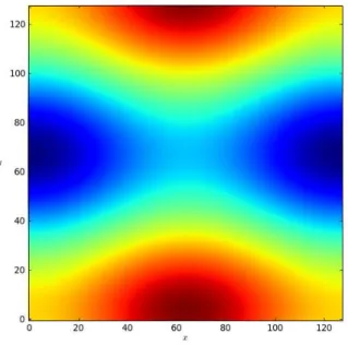
in(x, y) = ωeq(x) + β3N (x, y) , where β3= 0.01 andN represents the noise introduced before . In this way, we perturb the steady-state solution of the Kolmogorov flow. We choose an aspect ratio of 1/K = 1.1 and a viscosity of ϵ = 1× 10⁻³. The final physical time is T = 5000 . In figure 10, we plot the evolution of the vorticity ωϵ,σ at different times, obtained with our (DAMM)-scheme. We observe again the formation of a variety of flow patterns. Starting from the initial condition (panel (a)), the first stage of the instability is clearly observable in panel (b). Then, we observe during a long time a complex behaviour characterized by the formation of the coherent structures embedded in a sea of filaments (panel (c) and (d)). And finally, in the long-time asymptotics, the vorticity begins to saturate (panel (e)), and a steady state constituted by a pair of opposed vortices is obtained (panel (f)). For this final state, the external forcing term, which adds continuously kinetic energy to the system, is balanced by the viscous dissipation. Note that the wavy pattern obtained during the instability phase is very similar to the one obtained in the Taylor-Green instability (see figure 6).
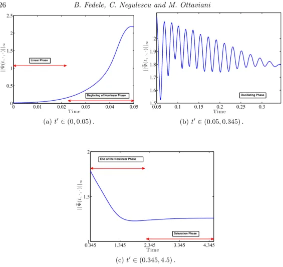
In order to understand in more details the Kolmogorov instability evolution, we plot in figure 11 three panels corresponding to the evolution of the discrete L∞-norm of *Ψ in three adjacent time-intervals. Dividing the curve in three plots allows one to distinguish more clearly all phases of the instability process. In panel (a), we observe the events which occur at short times. The linear phase, characterized by the relation between the aspect ratio and the growth rate, appears first. A nonlinear stage follows immediately, characterized by a strong growth of the norm. This nonlinear phase continues in panel (b) but with a complete different evolution. After the growth of the norm in panel (a), we
(a) (DAMM)-scheme, Initial condition . (b) (DAMM)-scheme, t = 50 .
(c) (DAMM)-scheme, t = 75 . (d) (DAMM)-scheme, t = 150 .
(e) (DAMM)-scheme, t = 1000 . (f) (DAMM)-scheme, t = 5000 .
Figure 10:(Kolmogorov flow with initial condition ωE
in). Vorticity field ωϵ,σat different physical
times, obtained with a viscosity of ϵ = 1e− 3 . Nx = Ny = 128, Nt = 50000, T = 5000,
0 0.01 0.02 0.03 0.04 0.05 0 0.5 1 1.5 2 2.5 Time || ! Ψ( t, · ,· )|| ∞ Linear Phase
Beginning of Nonlinear Phase
(a) t′∈ (0, 0.05) . 0.05 0.1 0.15 0.2 0.25 0.3 1.5 1.6 1.7 1.8 1.9 2 Time || ! Ψ( t, · ,· )|| ∞ Oscillating Phase (b) t′∈ (0.05, 0.345) . 0.3451 1.345 2.345 3.345 4.345 1.5 2 Time || ! Ψ( t, · ,· )|| ∞
End of the Nonlinear Phase
Saturation Phase
(c) t′∈ (0.345, 4.5) .
Figure 11: (Kolmogorov flow with initial condition ωinE). Discrete L∞-norm of !Ψ versus time
with ϵ = 1e− 3 , Nx= Ny= 64 , Nt= 45000,T = 4.5, σ = (∆x/Lx)2, and K = 1/1.1.
observe in panel (b) some damped oscillations and the decrease of the norm. This time-period corresponds to the merging and the filamentation of the vortices observed in figure 10. This oscillating phase is the most interesting one. Indeed, although the filamentation and the merging of the vortices lead to a very chaotic situation, the damped oscillations of the norm of *Ψ seem to have more ordered variations. Finally, during the third and longest part of the instability, the norm in panel (c) continues to decrease but without any oscillation (or very weak oscillations impossible to see) before it saturates. This saturation phase means that the new equilibrium is attained.
To end this section, we observe the relation between the vorticity and the stream function at the final time. Indeed, since the final pattern (panel (f)) in figure 10 does not evolve anymore, the Poisson bracket {ωϵ,σ, Ψϵ,σ
} should be of the same order as the term ϵ (∆ωϵ,σ+cos(x)) . Since we have chosen ϵ = 1.
×10−3, which is small, we should approach in this time asymptotic a functional relation between ωϵ,σ and Ψϵ,σ. In figure 12 (a), we show the final state of the stream function (−Ψϵ,σ) corresponding to the vorticity field plotted in the figure 10 (panel (f)). As expected, we observe that the vorticity and the stream-function have very similar patterns, with the vorticity more concentrated at the extremal points of the field. In figure 12 (b), the ωϵ,σ