• Aucun résultat trouvé

Computational vademecums for the real-time simulation of haptic collision between nonlinear solids

N/A
N/A
Protected

Academic year: 2021

Partager "Computational vademecums for the real-time simulation of haptic collision between nonlinear solids"

Copied!
36
0
0

Texte intégral

(1)

HAL Id: hal-01856396

https://hal.archives-ouvertes.fr/hal-01856396

Submitted on 10 Aug 2018

HAL is a multi-disciplinary open access

archive for the deposit and dissemination of sci-entific research documents, whether they are pub-lished or not. The documents may come from teaching and research institutions in France or

L’archive ouverte pluridisciplinaire HAL, est destinée au dépôt et à la diffusion de documents scientifiques de niveau recherche, publiés ou non, émanant des établissements d’enseignement et de recherche français ou étrangers, des laboratoires

Computational vademecums for the real-time simulation

of haptic collision between nonlinear solids

David González, Icíar Alfaro, Carlos Quesada, Elías Cueto, Francisco Chinesta

To cite this version:

David González, Icíar Alfaro, Carlos Quesada, Elías Cueto, Francisco Chinesta. Computational vade-mecums for the real-time simulation of haptic collision between nonlinear solids. Computer Methods in Applied Mechanics and Engineering, Elsevier, 2015, 283, pp.210-223. �10.1016/j.cma.2014.09.029�. �hal-01856396�

(2)

Computational vademecums for the real-time simulation

of haptic collision between nonlinear solids

I

David Gonz´aleza,b, Ic´ıar Alfaroa,b, Carlos Quesadaa, El´ıas Cuetoa,b,∗, Francisco Chinestac

aAragon Institute of Engineering Research (I3A), Universidad de Zaragoza. Maria de Luna 3, E-50018 Zaragoza, Spain.

bCIBER-BBN-Centro de Investigaci´on Biom´edica en Red en Bioingenier´ıa Biomateriales y Nanomedicina, Zaragoza, Spain.

cGEM UMR CNRS - Ecole Centrale de Nantes. 1 rue de la No¨e, BP 92101, F-44321 Nantes cedex 3, France.

Abstract

In this paper a novel strategy is presented for the real-time simulation of contact between non-linear deformable solids at haptic feedback rates. The proposed method is somehow related with the Voxmap Pointshell method for two deformable solids. Its novelty and crucial advantages over existing imple-mentations of this algorithm come from the intensive use of computational vademecums. These are in essence a pre-computed solution of a paramet-ric model in which every possible situation during the on-line phase of the method has been considered through the introduction of the appropriate pa-rameters. Such a high-dimensional parametric model is efficiently solved by using Proper Generalized Decompositions (PGD) and stored in memory as

IThis work has been partially supported by the Spanish Ministry of Science and Competitiveness, through grant number CICYT-DPI2011-27778-C02-01/02. Professor Chinesta is also supported by the Institut Universitaire de France. CIBER-BBN is an initiative funded by the VI National R&D&i Plan 2008-2011, Iniciativa Ingenio 2010, Consolider Program, CIBER Actions and financed by the Instituto de Salud Carlos III with assistance from the European Regional Development Fund.

Corresponding author

Email addresses: gonzal@unizar.es (David Gonz´alez), iciar@unizar.es (Ic´ıar Alfaro), cquesada@unizar.es (Carlos Quesada), ecueto@unizar.es (El´ıas Cueto), francisco.chinesta@ec-nantes.fr (Francisco Chinesta)

(3)

a set of vectors. The paper presents a thorough description of the developed algorithm together with some examples of its performance.

Keywords: Real time, contact, Model reduction, Proper Generalized Decomposition, Parametric models, Computational vademecums.

1. Introduction

Computational contact mechanics [66] constitutes nowadays a very active field of research due to its inherent difficulty, associated to the highly non-linear character of its models. But when we deal with non-non-linear solids and, in addition, real-time response is required, the problem becomes extremely burdensome and has generated a plethora of publications searching for a good compromise between accuracy and time to response, see for instance [8] [31] [10] [63], to name but a few of the available references.

Haptic peripherals have become very popular for augmented simulation in immersive environments, particularly for education purposes and games. They have been used notably in medical environments as an essential tool for the education in minimally invasive procedures [59] [60] [22] [40] [45] [18] [2] [49] and for training of complex industrial processes. In particular, aircraft and automobile industries have recently incorporated virtual reality to the design process to see whether a mechanical part could be located at a particular position in the plane in order to facilitate manufacturing and maintenance processes [7] [65] [57].

The main difficulty associated to haptic peripherals (those with force feedback) is that they need, to provide with a realistic sense of touch, a feedback response in the order of 500 Hz to 1 kHz. What this means in practice is that, very much like some 25 frames per second are needed in cinemas to provide the spectator with a continuous sensation of movement,

(4)

in haptic environments nearly one thousand simulations per second must be carried out to provide the user with a continuous sense of touch. 1 kHz is roughly the free-hand gesture frequency [21].

The reader will readily understand the difficulties associated with the simulation of non-linear solids (soft living tissues are frequently assumed to be hyperelastic, possibly with fiber reinforcement [30] [1]) under such astringent requirements. If, in addition, the possibility of contact between deformable solids is taken into account, the 1kHz constraint is even more difficult to fulfill.

Contact mechanics simulations under real-time restrictions have been tackled from a variety of approaches. One of the earliest and most popular is that of constructing Bounding Volume Hierarchies (BVH) [63], consisting in associating each node in a tree with a subset of the primitives (polygons, NURBS, etc.) defining the boundary of the object. Other approaches for real time include the use of stochastic contact detection [64], based on the assumption that the perceived realism of contact detection depends more of the real-time response than in the accuracy itself of the simulation.

One of the most popular families of real-time contact detection algorithms is based on the use of distance fields [13] [10]. Distance fields (level sets) constitute a very convenient way of representing very intricate geometries for contact detection, but has been traditionally considered as non-apt for real-time contact simulation between deformable solids, since the distance field must be updated according to the deformation of one of the solids [63]. If we restrict ourselves to the problem of real-time simulation of hyper-elastic solids, several approaches have been accomplished in the literature. Besides the obvious choice of considering a purely elastic material, but which renders very poor results in terms of visual realism in the presence of large

(5)

strains, the first approaches considered multi-resolution methods [36] [32]. Very popular in the last years are the methods based on the use of explicit finite element implementations [46], possibly based on parallelization by us-ing general-purpose Graphics Processus-ing Units (GPUs) [34] [59] [19]. Due to the inherent complexity of the objective, techniques based upon model order reduction methods have also recently reached some popularity. Among them, we can cite [47] [52] [48] [62] [61] [9]. In general, all these last references are based on the use of Proper Orthogonal Decomposition (POD) techniques [35] [41] [43], known also as Principal Component Analysis (PCA). These tech-niques employ an statistical treatment of the results obtained for complete, similar problems to the one at hand to construct a set of global, Ritz-like, basis functions that are optimal, with respecto to some measure, for the already solved, complete problems. They are then used for the problem un-der consiun-deration in the hope that, if the modifications with respect to the original problems are small, they will be also a good choice for it.

This approach presents some drawbacks. For instance, the choice of sim-ilar, complete problems, after which to obtain the set of global basis, is not an easy task [6]. In addition, model reduction methods loose many of their advantages if we deal with non-linear problems, since they need for the recon-struction of the full tangent stiffness matrix in order to obtain a consistent linearization of the problem. Although several approaches have been devel-oped to deal with this difficulty, no definitive response has been found [52] [14] [20].

As an alternative to POD techniques, Proper Generalized Decomposition (PGD) techniques can be seen as a sort of a priori model order reduction method, in the sense that no complete problem must be solved in order to obtain the set of global basis functions. The origin of PGD dates back to

(6)

the so-called radial loading approximation of the LArge Time INcrements (LATIN) method [37]. It consisted, essentially, of an space-time separated representation of the solution that very much resembles that of POD, but obtained completely in an a priori fashion.

Some years later, F. Chinesta employed a similar separated representation for the solution of high-dimensional problems arising from the kinetic theory of complex, non-Newtonian flows [3] [4]. Once both approaches have been identified as belonging to one single method for the model order reduction of PDEs, the field of application of PGD has grown exponentially. Just to cite some of the most recent survey papers, the interested reader can consult, for instance, [17] [15] [26] [16] [38] [29] [53].

Based on PGD, the authors have developed a series of computational vademecum approaches [16] for different physical problems such as thermal control of industrial furnaces [24] [25], dynamic, data-driven application sys-tems (DDDAS) [27], shape optimization [5] or computational surgery [50], to name a few. In essence, a computational vademecum (from the latin vade mecum, “goes with me”) is a sort of reference guide that helps engineers (or physicians) by abridging known solutions to given problems. One of the earli-est and most known examples is that of Bernoulli [12]. This concept has been translated by the authors to nowadays computational mechanics by comput-ing, off-line and once for life, parametric (and thus multi-dimensional) solu-tions for a given problem. This general, multi-dimensional solution (a sort of computational response surface or meta-model, if preferred) is then used (evaluated) on-line at very high feedback rates.

The main difficulty with computational vademecums is that they give rise to high-dimensional problems. It is well-known that, for mesh-based methods such as finite elements or finite differences, high-dimensional problems suffer

(7)

from the so-called curse of dimensionality [39], i.e., an exponential increase on the number of degrees of freedom with the number of dimensions of the space. This difficulty is at the very heart of the choice of PGD for such high-dimensional problems, since it assumes the solution as being expressed as a finite sum of separable functions.

In this paper a novel approach to the real-time simulation of contact between non-linear solids is presented. It is based on an intensive use of computational vademecums obtained off-line by means of PGD techniques. The developed technique can be seen as a particular instance of distance field methods, in which a general, high-dimensional distance field will be pre-computed off-line by taking the collision position as a parameter in the model. Thus, the most restrictive characteristic of distance field techniques will therefore be overcome, since there will be no need for distance field updating with the deformation of the solid.

In order to fully understand the developed methodology, a brief review of how to construct a computational vademecum by PGD techniques will be made in Section 2. The novel distance-field method will be presented in Section 3. In Section 4 examples of the performance of the proposed technique will be given. The paper is closed by some final remarks in Section

5.

2. A brief review of computational vademecums obtained by PGD techniques

As stated in the introduction, the main ingredient of the method here reported is the intensive use of computational vademecums [16]. In essence, the idea behind this method is to pre-compute off-line every possible situation (with the limitations that will be later clarified) that could be faced during

(8)

the on-line phase of the simulation.

Consider, as a starting point, the case of a vademecum in which we would like to store the displacement field u(x) of a non-linear (here, hyperelastic) solid Ω under the action of a force (assumed for the sake of simplicity as unitary and always acting in the vertical direction) at any point s of its boundary region Γ ⊂ Γt ⊂ Γ = ∂Ω. This renders a problem defined in general in R5 (u = u(x, s)), although if s is interpolated using nearest-neighbour interpolation, it can be seen as a one-dimensional parameter (the node in which the load is acting), rendering a problem in R4.

In the general case of an arbitrary force acting in any direction, the prob-lem would be stated so as to find the displacement field for any physical point x ∈ R3, for a load acting at any point of its boundary (a two-dimensional manifold in R3) and arbitrary values of its three components, thus t ∈ R3. This renders a problem defined in dimension 8.

Consider now the weak form of the equilibrium equations (balance of lin-ear momentum). Again, for the sake of simplicity, we omit inertia terms. For a detailed treatment of non-linear solid dynamics with the use of PGD and computational vademecums, the interested reader can consult [28]. Un-der these assumptions, the (doubly-) weak form of the problem, extended to the whole solid, Ω and the portion of its boundary which is accessible to load, ¯Γ ⊂ Γt, consists in finding the displacement u ∈ H1 such that for all u∗ ∈ H1 0: Z ¯ Γ Z Ω ∇su∗ : σdΩd¯Γ = Z ¯ Γ Z Γt2 u∗· tdΓd¯Γ (1)

where Γ = Γu∪ Γtrepresents the boundary of the solid, divided into essential and natural regions, and where Γt = Γt1∪ Γt2, i.e., regions of homogeneous and non-homogeneous, respectively, natural boundary conditions. Here, t = −ek· δ(x − s), where δ represents the Dirac-delta function and ek the unit

(9)

vector along the z-coordinate axis (we consider here, as mentioned before, and for the ease of exposition, a unit load directed towards the negative z axis of reference).

The Dirac-delta term is then regularized, and approximated by a trun-cated series of separable functions in the spirit of the PGD method, i.e.,

tj ≈ m X

i=1

fji(x)gji(s)

where m represents the order of truncation and fi

j, gji represent the j-th com-ponent of vectorial functions in space and boundary position, respectively.

PGD techniques allow to efficiently construct the computational vademe-cum u(x, s) by constructing, in an iterative way, an approximation to the solution in the form of a finite sum of separable functions [15]. Let us assume that the method has converged to a solution, at iteration n of this procedure,

unj(x, s) = n X k=1

Xjk(x) · Yjk(s), (2)

where the term uj refers to the j-th component of the displacement vector, j = 1, 2, 3 and functions Xk(x) and Yk(s) represent the separated functions used to approximate the unknown field, obtained in previous iterations of the PGD algorithm. At this stage, the objetive of PGD is to provide the solution with an improvement given by the (n + 1)-th term of the approximation,

un+1j (x, s) = unj(x, s) + Rj(x) · Sj(s), (3)

where R(x) and S(s) are the sought functions that improve the approxi-mation. In an equivalent manner, admissible variations of this displacement field will be given by

(10)

As can be noticed, even if the original problem is linear, PGD needs for the solution of a non-linear problem, i.e., to determine a product of functions, see Eq. (3). To this end, any of the possible linearization procedures could be employed. Traditionally, the authors have employed the simplest one, a fixed point, alternating directions algorithms that, although not being optimal, works in general very well. This strategy is briefly described hereafter.

2.1. Computation of S(s) assuming R(x) is known

In this case, following standard assumptions of variational calculus, we have

u∗j(x, s) = Rj(x) · Sj∗(s), (4)

or, equivalently, u∗(x, s) = R ◦ S∗. The symbol “◦” stands here for the so-called entry-wise, Hadamard or Schur multiplication for vectors. Once substituted into Eq. (1), gives

Z ¯ Γ Z Ω ∇s(R ◦ S∗) : C : ∇s n X k=1 Xk◦ Yk+ R ◦ S ! dΩd¯Γ = Z ¯ Γ Z Γt2 (R ◦ S∗) · m X k=1 fk◦ gk ! dΓd¯Γ,

or, equivalently (we omit obvious functional dependencies) Z ¯ Γ Z Ω ∇s(R ◦ S∗) : C : ∇s(R ◦ S)dΩd¯Γ = Z ¯ Γ Z Γt2 (R ◦ S∗) · m X k=1 fk◦ gk ! dΓd¯Γ − Z ¯ Γ Z Ω ∇s(R ◦ S∗) · RndΩd¯Γ, where Rn represents: Rn= C : ∇ sun.

(11)

Since the symmetric gradient operates on spatial variables only, we have: Z ¯ Γ Z Ω (∇sR ◦ S∗) : C : (∇sR ◦ S)dΩd¯Γ = Z ¯ Γ Z Γt2 (R ◦ S∗) · m X k=1 fk◦ gk ! dΓd¯Γ − Z ¯ Γ Z Ω (∇sR ◦ S∗) · RndΩd¯Γ

where all the terms depending on x are known and hence all integrals over Ω and Γt2 (the part of the natural boundary with non-homogeneous boundary conditions) can be computed to derive an equation to determine S(s).

2.2. Computation of R(x) assuming S(s) is known Equivalently, in this case, we have

u∗j(x, s) = R∗j(x) · Sj(s),

which, once substituted into Eq. (1), gives

Z ¯ Γ Z Ω ∇s(R∗◦ S) : C : ∇s n X k=1 Xk◦ Yk+ R ◦ S ! dΩd¯Γ = Z ¯ Γ Z Γt2 (R∗◦ S) · m X k=1 fk◦ gk ! dΓd¯Γ.

In this case all the terms depending on s (load position) can be integrated over ¯Γ, leading to a generalized elastic problem to compute function R(x).

As mentioned before, even if fixed-point algorithms do not have guaran-teed convergence properties, it is extremely unfrequent, in our experience, to find examples in which convergence is lost (see [17] and references therein). Other linearization strategies such as Newton-Raphson could also be equally employed [3] [4].

This development assumes implicitly small strain measures. For gen-eral, hyperelastic constitutive laws, large strain tensors (usually the Green-Lagrange tensor E) must be equally linearized. In the past, the authors have

(12)

tackled this linearization problem within the PGD approach in two different ways. In [50] an explicit approach was developed that renders, in general, very good results without stability problems. In [51] an approach was devel-oped based on the combined use of PGD and Asymptotic Numerical Methods (ANM). In this last approach, the solution u is expanded in terms of a power series of an arc-length parameter, providing a sort of continuation method in which there is no need of updating tangent stiffness matrices. Other ap-proaches such as the Discrete Empirical Interpolation Method [11] [14] could also be equally employed.

In general, following the aforementioned works, a strategy is followed in which enough terms in Eq. (2) so as to provide a norm of the residual below 10−5. Sometimes, given the strong limitations imposed by haptic response, further simplification of the PGD representation of the solution is needed. In that cases, the number of terms are restricted to those giving an accuracy always above 10%, computed with respect to full FE solutions of the same problem.

In general, we refer the interested reader to the previous works in the field [51] [50] [28] for a thorough discussion on the relationship between accuracy and number of terms in the PGD representation of the solution.

3. A distance-field method based on the use of computational vede-mecums

The method here developed assumes that a computational vademecum u(x, s) has already been computed for the solids under consideration. As mentioned before, this multi-dimensional solution provides a general solution for the displacement field in the solids under an arbitrary load acting on ¯Γ.

(13)

is modeled as a pointshell [10], i.e., a set of boundary points (assumed for simplicity identical to the boundary nodes of the solid model, although this is not strictly necessary) equipped with normals to the surface. As such, the algorithm is not symmetric, since the choice of which body is chosen to be equipped with the pointshell affects the final result of the simulation, albeit slightly. The other solid, Ω1, is in turn equipped with a signed distance field, see Fig. 1.

Figure 1: Sketch of the collision detection algorithm. Solid Ω1is equipped with a distance field, represented in the Figure, while solid Ω2 is represented, for collision detection pur-poses, as a pointshell, i.e., a collection of boundary nodes and normals to the surface (not represented for simplicity).

(14)

In our implementation, following closely [10], at every haptic cycle, con-tact penalty forces are determined by querying the points of Ω2 against the distance field associated to Ω1. Traditionally, this approach has been con-sidered not valid for haptic feedback requirements, if we deal with two de-formable solids, see [63]. This limitation is due to the need of updating the distance field along with the deformation of Ω1, which is not an easy task, even if the collision detection loop is not performed at every haptic cycle, as in [33]. In the approach here presented, there is no need for such an update, since a high-dimensional distance field is computed off-line that contains the distance fields for any deformed configuration of the solid.

Once collision has been detected, a force

F = −kcdn

is applied to both solids, provided that d is trilinearly interpolated from the distance field accompanying Ω1. kC is the contact penalty stiffness. The minus sign assumes that normals to Ω2point towards the interior of the solid, although this is completely arbitrary. Finally, n represents the normal to Ω2 in the deformed configuration. An equal force is applied to Ω1, regardless of its geometry, since we have no information on its normals to the surface. This very simple algorithm preserves continuity in the force computation, essential to perceive haptic response as realistic.

For very slender solids, large penetrations could eventually lead to de-creasing force values, provided that Ω2 crosses the medial axis of Ω1, see [10]. However, note that collision will be checked every millisecond. Except from very large solid velocities, this will likely never happen in fields such as computational surgery, for instance.

(15)

de-signed for one single punctual load, or at least for a fixed number of loads. In contact problems the position of contact, and therefore the number of contact-ing nodes is a priori unknown. In the results presented in Section 4, where non-linear constitutive equations and strain measures are inherent, a predic-tor of the result is obtained by simply applying superposition, i.e., a linear combination of the contacting load predicted by the vademecums associated to each contacting node.

This very simple approach results to be enough for many applications such as computational surgery [20], since visual realism is kept (no artificial gain of volume, as in purely elastic approaches, is obtained) and the human sense of touch is not able to detect the lack of accuracy generated in the resulting load transmitted by the haptic peripheral.

If more accuracy is needed, a correction can be added to this prediction by employing hyper reduction methods [54] [55] [56] [42]. In essence, the solu-tion is projected onto the subspace spanned by the PGD modes of the solusolu-tion (as in POD-based MOR) and the tangent stiffness matrix is evaluated only at a very limited number of elements of the mesh, typically some three times the number of modes considered. In our experiments, this approach has rendered excellent results, albeit not always necessary. This same rationale could be applied to the updating of the pre-computed distance field, although our expe-rience indicates that the force feedback produced by the predictor obtained by linear superposition provides sufficient accuracy. I general, the correction is not perceivable by the human sense of touch.

The use of the correction step could seem compromising real time re-sponses. However, it is important to notice that (i) only some elementary stiffness matrices are assembled (the global matrix is not singular because the global stiffness matrix appears pre- and post-multiplied by the matrix

(16)

contain-ing the reduced basis) [47]; (ii) because the iteration starts from the predic-tion, that is in general close to the final solupredic-tion, few correction iterations are needed; and (iii) only vector products are involved and all these can be computed simultaneously and in parallel by using GPUs, for example.

Even if the tests performed proved that surgical simulation applications do not need for the correction step, its consideration does not seem a great chal-lenge, and it will be integrated in our future works to extend the applicability of this strategy to domains other than computational surgery.

3.1. Computation of the distance field

The main ingredient of this algorithm is the distance field associated to the solid Ω1. Any method could be in principle valid for the computation of this field. The key novelty of the approach here presented is that a high-dimensional distance field

d = d(x, s)

for every load location s is computed off-line and stored in memory, very much in the spirit of computational vademecums. Here, x represents, by an abuse of notation, the coordinates of points belonging to the prism in which the distance field is computed, see Fig. 1. This prism, in general, does not need to be much bigger than the solid Ω1, see [63], to avoid storing a big number of nodal distance values. However, in the implementation here presented, the distance field must be such that every possible deformation state of Ω1 must lye within the prism. Once computed off-line and once for life, this distance field is evaluated for a particular load position s, that is, for any possible deformed configuration of the solid Ω1, thus giving a standard 3-d field for each load position, without the need of further updating.

Our implementation interpolates trilinearly the three physical coordinates and by nearest neighbors the s coordinate. This leads actually to a 4-d

(17)

dis-tance field d = d(x, y, z, s), where s represents the node number to which the load is associated. Test codes used Matlab’s griddedInterpolant algorithm [44] for a very fast evaluation of the distance field at a query point. Results are given in Section4on the performance of this technique. The distance field at nodal position of the grid could be computed by employing fast marching algorithms [58] or by simply employing the pdist Matlab function.

Remark 2. The brute force computation of the distance field is a feasible option if the number of dimensions of the problem (i.e., the number of pa-rameters of the solution) is kept relatively small. If this is not so, the number of distance values to compute grows exponentially with the number of dimen-sions. The authors are currently exploring the possibility of solving the fast marching equations [58] in parallel with the computation of the vademecum, Eqs. (2) and (3) in a PGD, separated way. In this manner, a vademecum could be obtained containing all the possible deformed configurations, each one attached to its distance field, both expressed in a separated form.

4. Numerical examples of performance

In what follows some examples have been selected to demonstrate the performance of the proposed method. Firstly, a Matlab [44] implementation of the algorithms was accomplished in order to check their validity. Once their performance had been assessed, a final implementation for the Geomagic Touch haptic device [23] was developed in order to test realism of the reaction forces, stability of the perceived touch, etc.

4.1. Contact between a beam and a rigid solid

To begin with, the simplest case of collision detection between a hypere-lastic (Saint Venant Kirchhoff) cantilever beam and a solid is considered. A

(18)

squared cross-section beam, with 40×40×400 mm, discretized with some 189 nodes, was considered. Young’s modulus was assumed to be 209000 MPa, while Poisson coefficient was set to 0.3. The beam is actuated by a vertical load of 106 N, that can be applied at any point of the boundary of the beam. If nearest-neighbor interpolation for the position of the load was assumed, a total of 170 different positions of this load could be encountered during the on-line phase of the simulation.

During the off-line phase of the calculation, a multidimensional solution is obtained for the displacement field of the beam, whose two first pairs of modes are shown in Fig. 2. Details of the PGD procedure for the solution of this parametric problem can be found at [51] or [50]. A total of 81 pairs of functions Xi and Yi (see Eq. (2)) were employed in this example, i.e., n = 81. Tests with only some 25 pairs also gave satisfactory results, with no perceptible loss of accuracy for the human eye. The off-line computation of this example takes roughly less than half an hour on a standard laptop.

Over this general solution u(x, s), a four-dimensional distance field d(x, s) is constructed. In this case, although the obvious choice would have been to equip the rigid solid with the distance field, to demonstrate the capabilities of the method the inverse solution has been preferred. Therefore, the distance field was attached to the deformable solid, the beam. The mesh to construct this distance field contained 42 × 26 × 61 × 170 nodes (i.e., more than eleven millions of degrees of freedom) along x, y, z and s (load position, considered as a one-dimensional array of nodal locations) directions, respectively.

A rigid block is also considered with which the beam gets into contact, see Fig. 3. All the possible load cases were tested and the time necessary to detect contact stored. On a Macbook Pro laptop equipped with an Intel Core i7 processor running at 3 GHz (8Gb DDR3 RAM at 1600 MHz) and

(19)

X Y Z F 0.4 0.38 0.36 0.34 0.32 0.3 0.28 0.26 0.24 0.22 0.2 0.18 0.16 0.14 0.12 0.1 0.08 0.06 0.04 0.02 (a) X Y Z F 0.3 0.25 0.2 0.15 0.1 0.05 0 -0.05 -0.1 -0.15 -0.2 -0.25 -0.3 -0.35 -0.4 -0.45 -0.5 (b) X Y Z F -0.02 -0.04 -0.06 -0.08 -0.1 -0.12 -0.14 -0.16 -0.18 -0.2 -0.22 -0.24 (c) X Y Z F 0.014 0.012 0.01 0.008 0.006 0.004 0.002 0 -0.002 -0.004 -0.006 -0.008 (d)

Figure 2: First two modes of the beam model, depending on the physical coordinates x (top) and load position s (bottom).

(20)

running Matlab [44] the results indicated that the time to contact detection was 0.0006223 ± 1.02122E − 07 seconds, well within the strong requirements of haptic contact feedback.

Figure 3: Collision between a beam and a rigid block for one of the 170 possible load locations in the model. The beam (red), the block (blue) and a slice of the distance field are depicted.

4.2. Contact between two hyperelastic beams

The fact that in the previous example a rigid solid was considered has no special implications on the complexity of the algorithm. If a deformable-deformable contact between two beams is now considered, the numbers re-main roughly the same, the complexity of the algorithm depending essentially on the number of nodes of the pointshell and the number of degrees of free-dom considered for the distance field. Both vademecums are essentially the

(21)

same, so that the computer cost of the off-line computations remains the same of the previous example.

The algorithm here presented is so powerful that it can be implemented on an html page running javascript, for instance, and still provide visual perception of interactivity when the beam is touched with the mouse on the screen, see Fig. 4. Contact iterations were limited to run in less than 100 ms, but the typical time to find collision was around 40 ms, still under the typical 25 frames per second of films.

Figure 4: Collision between two beams running on an html web page with embedded javascript. The red stroke indicates the position of the load actuating the blue beam.

The implementation of the same problem on a HP ProBook 6470b lap-top (Intel Core i7, with 8 Gb DDR3 PC3-12800 SDRAM running Ubuntu) equipped with a Geomagic Touch [23] haptic device also gave excellent re-sults, with no noticeable jumps in the perceived contact force, see Fig. 5.

(22)
(23)

4.3. Contact between two Stanford bunnies

In this example two Stanford bunnies were forced to contact each other in order to test the capabilities of the proposed technique. From the original STL file, a tetrahedral finite element model composed by 4285 nodes for each bunny was constructed, see Fig. 6. The total number of nodes in the pointshell (blue bunny in Fig. 6) was 3733. Bunnies were assumed to be modeled by a Kirchhoff-Saint Venant hyperelastic law with E = 2.0 · 107 MPa and ν = 0.3.

Figure 6: Collision between two Stanford bunnies. A slice of the distance field is also shown.

The vademecum for each bunny —they are identical for both bunnies— contained 143 modes. The cost of the off-line computation of these

(24)

vademe-cums was more than three hours on a Mac Pro computer running Matlab [44] and equipped with a 6-core Intel Xeon ES CPU (although no parallelization was accomplished) at 3.5 GHz and with 16 GB RAM, 1867 MHz DDR3.

The red bunny is actuated by the user, provoking a rigid-solid displace-ment until contact occurs with the blue one. Three different positions were tested. At position number 1, no collision was detected, and the total time employed by the proposed algorithm was 0.0007148 seconds. At position number 2, 36 contacting nodes were detected, while the total time employed for their location was 0.001611 seconds. Finally, at position number three, 427 nodes got into contact, and in this last case 0.0012811 seconds were necessary to detect them.

The deformed configuration of the bunnies after contact is depicted in Fig. 7.

Again, for complex, detailed models of intricate geometry, the proposed method is able to render feedback at rates on the order of 1 kHz, proving the validity of the assumptions made so far.

5. Conclusions

In this paper a method for the real-time detection of collision between deformable solids has been presented. Although inspired by existing algo-rithms, the novelty of the proposed technique lies in the use of computational vademecums, i.e., pre-computed solutions that are exploited on-line at very high feedback rates. Here, the proposed method has been successfully tested on a Geomagic Touch device needing for 1 kHz feedback rates.

These extremely efficient vademecums are previously computed with the help of Proper Generalized Decomposition strategies, in order to alleviate the burden associated with the curse of dimensionality, i.e., the exponential

(25)

Figure 7: Deformed configuration of the bunnies after contact. Only the undeformed configuration of the blue bunny is represented, for simplicity, in white.

(26)

increase of the number of degrees of freedom with the number of dimensions (parameters) of the problem. Solutions for the displacement field of different solids under arbitrary load locations are thus obtained and employed to com-pute four-dimensional distance fields to the boundary of the object. Collision with the second solid is detected by checking the position of its boundary nodes against this distance field. Boundary nodes lying at negative distance regions are then penalized to force them to avoid interpenetration.

The main advantage of the proposed method over existing algorithms is that it avoids the need of updating the distance field with the deformation of the reference solid. Since any deformation of the solid has been parametrized previously by PGD and stored efficiently as a set of one-dimensional vectors, with the distance function associated to each deformed configuration, no need for on-line updating of the distance field results. This allows for a more detailed mesh for the computation of the distance field or, equivalently, for a more detailed geometric approximation of the pointshell in the second solid. So far only collision detection has been accomplished within this algo-rithm, although be strongly believe that a generalization of the proposed technique is possible for frictional contact. This constitutes nowadays our main effort of research, whose results will be presented elsewhere.

References

[1] V. Alastrue, B. Calvo, E. Pena, and M. Doblare. Biomechanical model-ing of refractive corneal surgery. Journal of Biomechanical Engineermodel-ing- Engineering-Trasactions of the ASME, 128:150–160, 2006.

[2] Iciar Alfaro, David Gonzalez, Felipe Bordeu, Adrien Leygue, Amine Ammar, Elias Cueto, and Francisco Chinesta. Real-time in silico

(27)

exper-iments on gene regulatory networks and surgery simulation on handheld devices. Journal of Computational Surgery, 1(1):2194–3990, 2014.

[3] A. Ammar, B. Mokdad, F. Chinesta, and R. Keunings. A new fam-ily of solvers for some classes of multidimensional partial differential equations encountered in kinetic theory modeling of complex fluids. J. Non-Newtonian Fluid Mech., 139:153–176, 2006.

[4] A. Ammar, B. Mokdad, F. Chinesta, and R. Keunings. A new family of solvers for some classes of multidimensional partial differential equa-tions encountered in kinetic theory modeling of complex fluids. part ii: transient simulation using space-time separated representations. J. Non-Newtonian Fluid Mech., 144:98–121, 2007.

[5] Amine Ammar, Antonio Huerta, Francisco Chinesta, El´ıas Cueto, and Adrien Leygue. Parametric solutions involving geometry: A step to-wards efficient shape optimization. Computer Methods in Applied Me-chanics and Engineering, 268(0):178 – 193, 2014.

[6] D. Amsallem and Ch. Farhat. An Interpolation Method for Adapting Reduced-Order Models and Application to Aeroelasticity. AIAA Jour-nal, 46:1803–1813, 2008.

[7] Aiert Amundarain, Diego Borro, Alex Garc´ıa-Alonso, Jorge Juan Gila, Luis Mateya, and Joan Savall. Virtual reality for aircraft engines main-tainability. M´ecanique et Industries, 5(2):121–127, 2004.

[8] Jernej Barbiˇc and Doug James. Time-critical distributed contact for 6-DoF haptic rendering of adaptively sampled reduced deformable mod-els. In Metaxas, D and Popovic, J, editor, SYMPOSIUM ON COM-PUTER ANIMATION 2007: ACM SIGGRAPH/ EUROGRAPHICS

(28)

SYMPOSIUM PROCEEDINGS, pages 171–180, 1515 BROADWAY, NEW YORK, NY 10036-9998 USA, 2007. ACM SIGGRAPH; Eurog As-soc, ASSOC COMPUTING MACHINERY. Symposium on Computer Animation, San Diego, CA, AUG 03-04, 2007.

[9] Jernej Barbiˇc and Doug L. James. Real-time subspace integration for St. Venant-Kirchhoff deformable models. ACM Transactions on Graphics (SIGGRAPH 2005), 24(3):982–990, August 2005.

[10] Jernej Barbiˇc and Doug L. James. Six-dof haptic rendering of con-tact between geometrically complex reduced deformable models. IEEE Transactions on Haptics, 1(1):39–52, 2008.

[11] M Barrault, Y Maday, NC Nguyen, and AT Patera. An ‘empirical interpolation’ method: application to efficient reduced-basis discretiza-tion of partial differential equadiscretiza-tions. Comptes Rendus Mathematique, 339(9):667–672, NOV 1 2004.

[12] C. Bernoulli. Vademecum des Mechanikers. Cotta, 1836.

[13] R. Bridson, S. Marino, and R. Fedkiw. Simulation of clothing with folds and wrinkles. In Proceedings of the 2003 ACM SIG-GRAPH/Eurographics Symposium on Computer Animation, SCA ’03, pages 28–36, Aire-la-Ville, Switzerland, Switzerland, 2003. Eurograph-ics Association.

[14] Saifon Chaturantabut and Danny C. Sorensen. Nonlinear model re-duction via discrete empirical interpolation. SIAM J. Sci. Comput., 32:2737–2764, September 2010.

[15] F. Chinesta, A. Ammar, and E. Cueto. Recent advances in the use of the Proper Generalized Decomposition for solving multidimensional

(29)

models. Archives of Computational Methods in Engineering, 17(4):327– 350, 2010.

[16] F. Chinesta, A. Leygue, F. Bordeu, J.V. Aguado, E. Cueto, D. Gonza-lez, I. Alfaro, A. Ammar, and A. Huerta. PGD-Based Computational Vademecum for Efficient Design, Optimization and Control. Archives of Computational Methods in Engineering, 20(1):31–59, 2013.

[17] Francisco Chinesta, Pierre Ladeveze, and Elias Cueto. A short review on model order reduction based on proper generalized decomposition. Archives of Computational Methods in Engineering, 18:395–404, 2011.

[18] St´ephane Cotin, Herv´e Delingette, and Nicholas Ayache. Real-time elas-tic deformations of soft tissues for surgery simulation. In Hans Hagen, editor, IEEE Transactions on Visualization and Computer Graphics, volume 5 (1), pages 62–73. IEEE Computer Society, 1999.

[19] Hadrien Courtecuisse, J´er´emie Allard, Pierre Kerfriden, St´ephane P.A. Bordas, St´ephane Cotin, and Christian Duriez. Real-time simulation of contact and cutting of heterogeneous soft-tissues. Medical Image Anal-ysis, 18(2):394 – 410, 2014.

[20] Elias Cueto and Francisco Chinesta. Real time simulation for com-putational surgery: a review. Advanced Modeling and Simulation in Engineering Sciences, 1(1):11, 2014.

[21] H. Delingette and N. Ayache. Soft tissue modeling for surgery simula-tion. In N. Ayache, editor, Computational Models for the Human Body, Handbook of Numerical Analysis (Ph. Ciarlet, Ed.), pages 453–550. El-sevier, 2004.

(30)

[22] Herve Delingette and Nicholas Ayache. Hepatic surgery simulation. Communications of the ACM, 48:31–36, February 2005.

[23] Geomagic. OpenHaptics Toolkit. 3D systems - Geomagic solutions, 430 Davis Drive, Suite 300 Morrisville, NC 27560 USA, 2013.

[24] Ch. Ghnatios, F. Chinesta, E. Cueto, A. Leygue, A. Poitou, P. Breitkopf, and P. Villon. Methodological approach to efficient modeling and op-timization of thermal processes taking place in a die: Application to pultrusion. Composites Part A: Applied Science and Manufacturing, 42(9):1169 – 1178, 2011.

[25] Ch. Ghnatios, F. Masson, A. Huerta, A. Leygue, E. Cueto, and F. Chinesta. Proper generalized decomposition based dynamic data-driven control of thermal processes. Computer Methods in Applied Me-chanics and Engineering, 213–216(0):29 – 41, 2012.

[26] D. Gonzalez, A. Ammar, F. Chinesta, and E. Cueto. Recent advances on the use of separated representations. International Journal for Nu-merical Methods in Engineering, 81(5), 2010.

[27] D. Gonzalez, F. Masson, F. Poulhaon, E. Cueto, and F. Chinesta. Proper generalized decomposition based dynamic data driven inverse identifica-tion. Mathematics and Computers in Simulation, 82:1677–1695, 2012.

[28] David Gonzalez, Elias Cueto, and Francisco Chinesta. Real-time direct integration of reduced solid dynamics equations. Internatinal Journal for Numerical Methods in Engineering, accepted, 2014.

[29] Ch. Heyberger, P.-A. Boucard, and D. Neron. A rational strategy for the resolution of parametrized problems in the {PGD} framework.

(31)

Com-puter Methods in Applied Mechanics and Engineering, 259(0):40 – 49, 2013.

[30] G. A. Holzapfel and T. C. Gasser. A new constitutive framework for arterial wall mechanics and a comparative study of material models. Journal of Elasticity, 61:1–48, 2000.

[31] D. L. James. Bd-tree: Output-sensitive collision detection for reduced deformable models. ACM Transactions on Graphics, 23:393–398, 2004.

[32] Doug L. James and Dinesh K. Pai. Multiresolution green’s function methods for interactive simulation of large-scale elastostatic objects. ACM Trans. Graph., 22(1):47–82, January 2003.

[33] Lenka Jeˇr´abkov´a and Torsten Kuhlen. Stable cutting of deformable ob-jects in virtual environments using xfem. IEEE Comput. Graph. Appl., 29(2):61–71, March 2009.

[34] Grand Roman Joldes, Adam Wittek, and Karol Miller. Real-time non-linear finite element computations on {GPU} – application to neuro-surgical simulation. Computer Methods in Applied Mechanics and En-gineering, 199(49–52):3305 – 3314, 2010.

[35] K. Karhunen. Uber lineare methoden in der wahrscheinlichkeitsrech-nung. Ann. Acad. Sci. Fennicae, ser. Al. Math. Phys., 37, 1946.

[36] Jung Kim, Changmok Choi, Suvranu De, and Mandayam A. Srinivasan. Virtual surgery simulation for medical training using multi-resolution organ models. The International Journal of Medical Robotics and Com-puter Assisted Surgery, 3(2):149–158, 2007.

(32)

[37] P. Ladeveze. Nonlinear Computational Structural Mechanics. Springer, N.Y., 1999.

[38] P. Ladeveze, J.-C. Passieux, and D. Neron. The latin multiscale compu-tational method and the proper generalized decomposition. Computer Methods in Applied Mechanics and Engineering, 199(21-22):1287 – 1296, 2010.

[39] R. B. Laughlin and David Pines. The theory of everything. Proceedings of the National Academy of Sciences, 97(1):28–31, 2000.

[40] Yi-Je Lim and Suvranu De. Real time simulation of nonlinear tissue response in virtual surgery using the point collocation-based method of finite spheres. Computer Methods in Applied Mechanics and Engineer-ing, 196:3011–3024, 2007.

[41] M. M. Lo`eve. Probability theory. The University Series in Higher Math-ematics, 3rd ed. Van Nostrand, Princeton, NJ, 1963.

[42] E. Lopez, E. Abisset, Ch. Ghnatios, Ch. Binetruy, and F. Chinesta. To-wards real time thermal homogenization of heterogeneous microstruc-tures. In 3rd International Conference on Computational Methods for Thermal Problems, 2014.

[43] E. N. Lorenz. Empirical Orthogonal Functions and Statistical Weather Prediction. MIT, Departement of Meteorology, Scientific Report Num-ber 1, Statistical Forecasting Project, 1956.

[44] MATLAB. version 8.1.0.604 (R2013a). The MathWorks Inc., Natick, Massachusetts, 2013.

(33)

[45] U. Meier, O. Lopez, C. Monserrat, M. C. Juan, and M. Alcaniz. Real-time deformable models for surgery simulation: a survey. Computer Methods and Programs in Biomedicine, 77(3):183–197, 2005.

[46] Karol Miller, Grand Joldes, Dane Lance, and Adam Wittek. Total la-grangian explicit dynamics finite element algorithm for computing soft tissue deformation. Communications in Numerical Methods in Engi-neering, 23(2):121–134, 2007.

[47] S. Niroomandi, I. Alfaro, E. Cueto, and F. Chinesta. Real-time de-formable models of non-linear tissues by model reduction techniques. Computer Methods and Programs in Biomedicine, 91(3):223 – 231, 2008.

[48] S. Niroomandi, I. Alfaro, E. Cueto, and F. Chinesta. Accounting for large deformations in real-time simulations of soft tissues based on reduced-order models. Computer Methods and Programs in Biomedicine, 105(1):1–12, 2012.

[49] S. Niroomandi, I. Alfaro, D. Gonzalez, E. Cueto, and F. Chinesta. Real-time simulation of surgery by reduced-order modeling and x-fem tech-niques. International Journal for Numerical Methods in Biomedical En-gineering, 28(5):574–588, 2012.

[50] S. Niroomandi, D. Gonz´alez, I. Alfaro, F. Bordeu, A. Leygue, E. Cueto, and F. Chinesta. Real-time simulation of biological soft tissues: a PGD approach. International Journal for Numerical Methods in Biomedical Engineering, 29(5):586–600, 2013.

[51] S. Niroomandi, D. Gonzalez, I. Alfaro, E. Cueto, and F. Chinesta. Model order reduction in hyperelasticity: a proper generalized decomposition

(34)

approach. International Journal for Numerical Methods in Engineering, 96(3):129–149, 2013.

[52] Siamak Niroomandi, Iciar Alfaro, Elias Cueto, and Francisco Chinesta. Model order reduction for hyperelastic materials. International Journal for Numerical Methods in Engineering, 81(9):1180–1206, 2010.

[53] Anthony Nouy. A priori model reduction through Proper Generalized Decomposition for solving time-dependent partial differential equations. COMPUTER METHODS IN APPLIED MECHANICS AND ENGI-NEERING, 199(23-24):1603–1626, 2010.

[54] D. Ryckelynck. A priori hyperreduction method: an adaptive approach. Journal of Computational Physics, 202(1):346–366, 2005.

[55] D. Ryckelynck. Hyper-reduction of mechanical models involving internal variables. International Journal for Numerical Methods in Engineering, 77(1):75–89, 2008.

[56] D Ryckelynck, L Hermanns, F Chinesta, and E Alarcon. An effi-cient ‘a priori’ model reduction for boundary element models. ENGI-NEERING ANALYSIS WITH BOUNDARY ELEMENTS, 29(8):796– 801, AUG 2005.

[57] Mikel Sagardia and Thomas Hulin. Fast and accurate distance, penetra-tion, and collision queries using point-sphere trees and distance fields. In ACM SIGGRAPH 2013 Posters, SIGGRAPH ’13, pages 83:1–83:1, New York, NY, USA, 2013. ACM.

(35)

[59] Z.A. Taylor, M. Cheng, and S. Ourselin. High-speed nonlinear finite element analysis for surgical simulation using graphics processing units. Medical Imaging, IEEE Transactions on, 27(5):650 –663, may 2008.

[60] Z.A. Taylor, O. Comas, M. Cheng, J. Passenger, D.J. Hawkes, D. Atkin-son, and S. Ourselin. On modelling of anisotropic viscoelasticity for soft tissue simulation: Numerical solution and GPU execution. Medi-cal Image Analysis, 13(2):234 – 244, 2009. Includes Special Section on Functional Imaging and Modelling of the Heart.

[61] Z.A. Taylor, S. Crozier, and S. Ourselin. A reduced order explicit dy-namic finite element algorithm for surgical simulation. Medical Imaging, IEEE Transactions on, 30(9):1713 –1721, sept. 2011.

[62] Z.A. Taylor, S. Ourselin, and S. Crozier. A reduced order finite ele-ment algorithm for surgical simulation. In Engineering in Medicine and Biology Society (EMBC), 2010 Annual International Conference of the IEEE, pages 239 –242, 31 2010-sept. 4 2010.

[63] M. Teschner, S. Kimmerle, B. Heidelberger, G. Zachmann, L. Raghu-pathi, A. Fuhrmann, M.-P. Cani, F. Faure, N. Magnenat-Thalmann, W. Strasser, and P. Volino. Collision detection for deformable objects. Computer Graphics Forum, 24(1):61–81, 2005.

[64] S. Uno and M. Slater. The sensitivity of presence to collision response. In Proceedings of the 1997 Virtual Reality Annual International Symposium (VRAIS ’97), VRAIS ’97, pages 95–, Washington, DC, USA, 1997. IEEE Computer Society.

[65] Ming Wan and William A. McNeely. Quasi-static approximation for 6 degrees-of-freedom haptic rendering. In Proceedings of the 14th IEEE

(36)

Visualization 2003 (VIS’03), VIS ’03, pages 34–, Washington, DC, USA, 2003. IEEE Computer Society.

Figure

Figure 1: Sketch of the collision detection algorithm. Solid Ω 1 is equipped with a distance field, represented in the Figure, while solid Ω 2 is represented, for collision detection  pur-poses, as a pointshell, i.e., a collection of boundary nodes and nor
Figure 2: First two modes of the beam model, depending on the physical coordinates x (top) and load position s (bottom).
Figure 3: Collision between a beam and a rigid block for one of the 170 possible load locations in the model
Figure 4: Collision between two beams running on an html web page with embedded javascript
+4

Références

Documents relatifs

L’archive ouverte pluridisciplinaire HAL, est destinée au dépôt et à la diffusion de documents scientifiques de niveau recherche, publiés ou non, émanant des

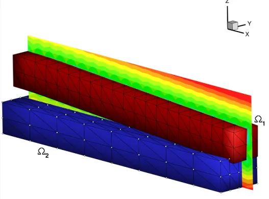
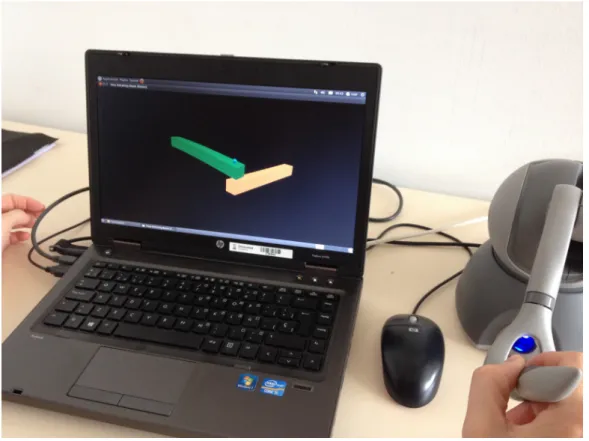
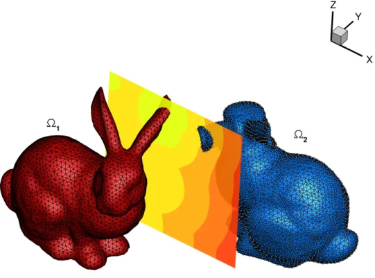
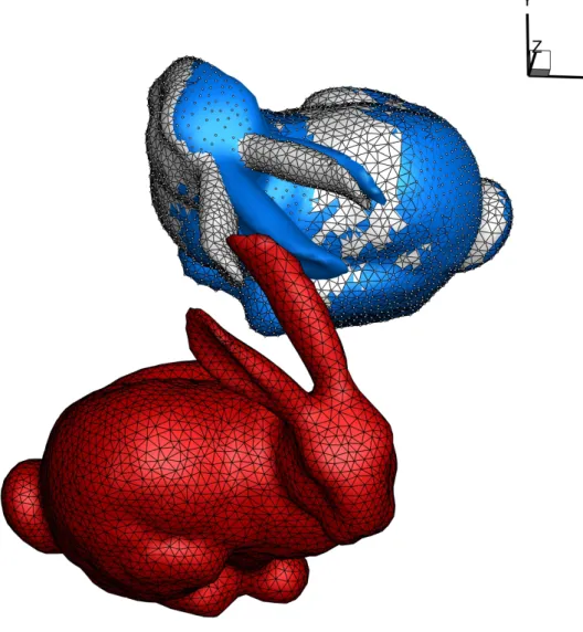
It relies on a high efficiency collision detection algorithm for deformable surface meshes, combined with an efficient FEM-based simulation of deformable surfaces enabling

The steps of the methodology are the fol- lowing: (1) introduction of a family of Prior Algebraic Stochastic Model (PASM), (2) identification of an optimal PASM in the

Those characteristics include the distinction between static and dynamic occurring tasks, bring out tasks whose execution time may change over the time and determine the number

L’archive ouverte pluridisciplinaire HAL, est destinée au dépôt et à la diffusion de documents scientifiques de niveau recherche, publiés ou non, émanant des

Water vapor advection and the subsequent formation of clouds quite differ when we compare these brand new high resolution simulations and the usual lower resolution ones at 64 per

Using the repertory grid and a Delphi survey to develop quality criteria genuine to humanities research, we were able to identify indicators that also reflect the ‘traditional’

Two implementations are currently developed in parallel; one based on a relational database (postgres/postgis) and a second one based on Flink (Salmon et al., 2015) to cope