Joint sink and route selection for anycast communications in wireless sensor networks

HAL Id: hal-01790291

https://hal.archives-ouvertes.fr/hal-01790291

HAL is a multi-disciplinary open access archive for the deposit and dissemination of sci-entific research documents, whether they are pub-lished or not. The documents may come from teaching and research institutions in France or abroad, or from public or private research centers.

L’archive ouverte pluridisciplinaire HAL, est destinée au dépôt et à la diffusion de documents scientifiques de niveau recherche, publiés ou non, émanant des établissements d’enseignement et de recherche français ou étrangers, des laboratoires publics ou privés.

communications in wireless sensor networks

Nancy Rachkidy, Alexandre Guitton, Michel Misson

To cite this version:

Nancy Rachkidy, Alexandre Guitton, Michel Misson. Joint sink and route selection for anycast com-munications in wireless sensor networks. Introduction to routing issues, 2012. �hal-01790291�

Joint sink and route selection for anycast communications in

wireless sensor networks

LIMOS CNRS, Clermont Université Campus des Cézeaux, 63 173 Aubière Cedex, France

Abstract

Most wireless sensor networks are used for monitoring purposes, where some nodes sense the environment and forward their measurements to an entity called the sink. Nodes around the sink tend to have their energy depleted faster than other nodes in the network, as they have the burden of forwarding the measurements from all the nodes. Thus, the current trend in wireless sensor networks is to consider networks with several sinks. In this context, anycast communications are important: each node producing traffic has to send its measurements to any available sink, generally to the closer one.

In this chapter, we aim at reducing the congestion in the whole network by jointly selecting sinks and routes from sources to sinks. We show that considering the two problems separately results into low performance. After proving that the joint sink and route selection problem is NP-hard, we propose a mixed integer linear program in order to obtain optimal solutions. Then, we propose a centralized mechanism that selects sinks and routes packets with reasonable performance (compared to the optimal solutions) and control overhead. Our approach contributes to balance the generated traffic in the network by considering special nodes called pivots. Our mechanism is validated by extensive simulations on generic network topologies. Then, we show how this mechanism can be distributed, using only a limited knowledge.

1

Introduction

In the past few years, wireless sensor networks (WSNs) have been used in several monitoring (He et al., 2004) and tracking (Juang et al., 2002) applications. WSNs are composed of cheap battery-powered devices that are able to sense the environment, to collect the measurements, and to send the collected data in a hop-to-hop wireless manner to a data-gathering station, called the sink. The sink usually has a large memory capacity, and sometimes does not even have energy limitations, contrarily to the sensor nodes. The sink has several roles: it can store historical data, analyze the data to detect discrepancies or emergency situations, or act as a gateway providing connectivity with a wired network.

In a typical monitoring application (such as in forest monitoring), a WSN is deployed over a large area. Sensor nodes sense the environment periodically and report their measurements to one sink. High contention is likely to occur around the sink, as it is where the paths from each source converge. In such a scenario, the network might experience high latency and high packet loss rate, which is not acceptable in an emergency scenario. Thus, it is very important to design communication protocols that can reduce the latency and the loss rate.

Addition-ally, high loss rate might yield to a large number of retransmissions, which causes congestion. Minimizing the congestion is therefore an important issue.

As the traffic converges to the sink, nodes close to the sink consume their energy faster than farther nodes. If the nodes close to the sink have their energy depleted, the sink is not able to receive any data and gets disconnected from the network. A solution to this problem is to deploy several sinks. When the traffic is balanced among several sinks, the network lifetime can be significantly increased.

The paradigm of anycast communications, also termed as one-to-any communications, becomes very im-portant in a network with multiple sinks: when a sensor node produces data, it has to send them to any available sink. An example of a strategy is to route data to the closest sink. Assuming that the sources and the sinks are uniformly distributed in the network, this is expected to balance the energy consumption. Another example of a sink selection strategy is to choose for each source a random sink.

In this chapter, we focus on optimizing the selection of the sinks by considering them jointly with the routes. We propose a mechanism which is able to minimize interferences and to reduce the congestion areas between the different paths. This mechanism is first described as centralized (El Rachkidy et al., 2010), and then

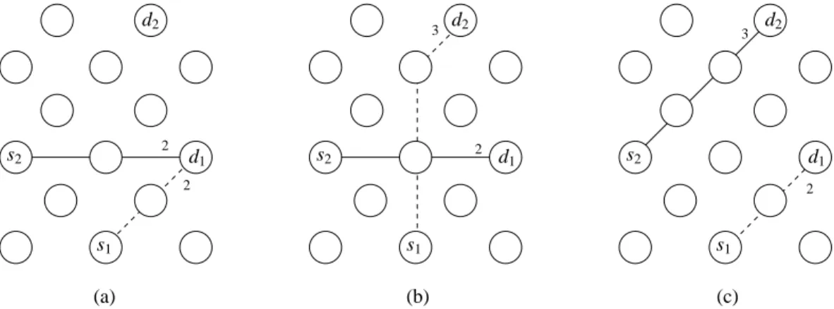
as distributed. Figure 1 shows an example of a topology with two sources s1 and s2 and two destinations d1and

d2, according to three sink selection strategies. On part (a) of the figure, each source is connected to the closest

sink, which generates contention around sink d1. On part (b), each source is connected to a different sink in order

to balance the sink load. However, some nodes of the networks are on the two paths(s1, d2) and (s2, d1), which

yields to contention on the wireless medium around those nodes. On part (c), the two paths(s1, d1) and (s2, d2)

are distant from each other. The traffic transmitted on one path has little impact on the traffic transmitted on the other path. This third sink selection strategy can only be achieved when considering the sink selection and the routing process simultaneously.

2 2 2 2 3 ₃ s1 s1 s1 s2 s2 s2 d1 d1 d1 d2 d2 d2 (a) (b) (c)

Figure 1: To minimize interferences and reduce congestion on the paths from each source to a sink,

sinks and paths have to be considered jointly.

The remainder of this chapter is as follows. In Section 2, we describe the related work and some existing sink selection strategies. Section 3 defines the problem of finding distant paths for a set of anycast communica-tions. We prove that this problem is NP-hard, and we propose an integer linear formulation in order to obtain optimal solutions. Section 4 gives details on the centralized version of our mechanism. Section 5 describes the simulation environment and settings, and provides the simulation results we obtained. Section 6 describes how the mechanism can be distributed. Finally, we conclude our work in Section 7.

2

State of the art

In this section, we focus on four main topics related to this work: the deployment of multiple sinks, the anycast paradigm where sources can send data to any sink, the use of multipaths in wireless routing protocols, and some existing sink selection strategies.

2.1 Multi-sink deployment

Recently, interest is emerging towards deployments with multiple sinks in order to improve the network life-time and to ensure a fair delivery of data among sinks (Kim et al., 2005; Oyman & Ersoy, 2004), where each sink has identical functional capabilities. Deploying several sinks in the network helps in balancing the traf-fic among nodes, and the congestion around each sink is reduced: the nodes surrounding the sinks are less overloaded and less used, their energy is less quickly depleted and thus, the network lifetime is extended. Another advantage of deploying multiple sinks is to improve the data gathering by reducing the communi-cation delay from sources to sinks (Chang & Tassiulas, 2007; Buratti et al., 2006) or the total communicommuni-cation cost (Kalantari & Shayman, 2006). Indeed, a network with a single sink might yield to large delays since some nodes are used by most of the paths, and thus several congested links might appear in the network. These con-gested links cause an increase in the loss rate, and retransmissions become required. A network with several sinks allows to build disjoint paths from sources to sinks, and reduce congestion.

2.2 Anycast communications

Anycast is a one-to-any communication paradigm where a source communicates with a single sink, chosen among a set of possible sinks. It has been shown that the lifetime of a WSN can be increased by deploying several sinks, and accessing them using an anycast protocol (Hu et al., 2005; Thepvilojanapong et al., 2005). Indeed, anycast communications can lead to significant energy savings in comparison to traditional protocols (such as Direct Diffusion (Intanagonwiwat et al., 2003)), improve the network scalability, and handle moderate sink mobility. In (Kim et al., 2008), the authors showed that anycast forwarding schemes can substantially reduce the one-hop

delay1 over traditional schemes, especially when nodes are densely deployed, as is the case for many WSN

applications. However, the reduction in the one-hop delay may not necessarily lead to a reduction in the expected end-to-end delay experienced by a packet, because the first candidate node that wakes up may not have a small end-to-end delay to the sink.

2.3 Multipath routing

Multipath routing is a feature that enables a source to send packets to a destination through multiple paths at the same time. The main advantage of this feature is to improve the reliability of the packet delivery: even if one path becomes blocked or delayed due to a node failure for instance, the destination is still able to receive packets from the source as long as at least one path is active. Using multipath also helps balancing the energy consumption among the nodes of the network, and therefore extends network lifetime. Most of the multipath routing protocols are based on classic on-demand single path routing methods (Marina & Das, 2001; Lee & Gerla, 2001).

Disjoint multipath routing methods try to determine disjoint paths, i.e., paths that do not have nodes or links in common. As stated in (Pearlman et al., 2000), using disjoint multipaths does not remove the poten-tial for collisions, and may therefore result into large packet loss rates and reduced data transmission perfor-mance. The main reason is that wireless transmissions might interfere communications between distant nodes.

1_{The one-hop delay is defined as the time required to transmit data to a neighbor. If neighbors have their own sleeping schedule,}

In (Saha et al., 2003), the authors aim to find zone-disjoint multipaths using directional antennas. A promising approach is described in (Wang et al., 2009), where authors proposed an energy efficient and collision aware dis-joint multipath routing algorithm. The flooding required to determine such paths is limited to nodes close to the main discovered route.

In this chapter, we do not use multipath to route traffic from a source to a sink. We rather aim to determine a collection of paths (one per source-sink pair) that are distant from each other. However, as shown in Section 3, the problems of finding two disjoint multipaths between one source-sink pair, or two disjoint paths between two source-sink pairs, are closely related.

In (El Rachkidy et al., 2009), we proposed a probabilistic proactive routing protocol based on pivots and called PiRAT. When an emergency situation occurs, several geographically close sensors might produce alarm messages that have to be forwarded to a sink. The paths followed by all the alarms might become congested and several alarm packets might be dropped. By selecting randomly distant pivot nodes for each source, PiRAT is able to reduce the congested areas and to improve the network performance in terms of delay and packet loss. This use of multipaths allows diversity in routing and avoids congested areas in the network, which contributes to balance the traffic load and the energy consumption between nodes. Figure 2 shows the usage of links in PiRAT. The sources are the nine nodes at the bottom left-hand corner, and the destination is at the top right-hand corner. The pivot nodes selected by the sources are colored in gray. It can be noticed that routes from the sources to the sinks avoid the central area in order to reduce congestion (the shortest path uses the central area). The probabilistic nature of PiRAT can be seen as each node uses several paths to reach a given destination (the destination being either the pivot node or the sink). Although several nodes are involved in the routing process, the amount of transmitted packet per node is small. This leads to reduce the overloaded paths and balance the energy consumption of the nodes. This phenomenon greatly improves the network lifetime. However, PiRAT is not able to reduce the congestion around the sink.

2.4 Existing sink selection strategies

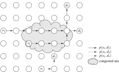
In the random sink selection strategy (RSSS), sinks are randomly chosen (Shukla & Menghanathan, 2005) by the sources. Packets are routed using the shortest path from each source to its selected sink. Generally, this strategy does not perform well in terms of delay and packet loss, as congestion might occur in several areas of the network. Congestion also increases the delay due to retransmission attempts.

Figure 3 shows an example of RSSS on a grid network with three sources (s1, s2, s3) and three sinks

(d1, d2, d3). For each source, a random sink is associated. It can be noticed that the three paths are not distant, and

some paths even intersect, which yields to a large congested area in the network. This congested area negatively impacts the network performance in terms of loss rate and end-to-end delay.

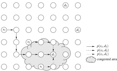
In the closest sink selection strategy (CSSS), each source is connected to its closest sink (Luo et al., 2008), in terms of geographical distance or, more generally, hop count. With this strategy, several sources can have the same sink. Thus, the area around such sinks might be congested, leading nodes in these areas to deplete their energy faster than the other nodes in the network, and also reducing the performance due to congestion.

Figure 4 shows an example of CSSS on the same graph. With CSSS, each source chooses its closest sink. In this example, all the sources choose as destination sink d1. This strategy yields to a congestion area around

d1. Note that when an event occurs, it is frequent that several sources located in a limited region start producing

0 1 2 3 4 5 6 7 8 9 10 11 12 13 14 15 16 17 18 19 20 21 22 23 24 25 26 27 28 29 30 31 32 33 34 35 36 37 38 39 40 41 42 43 44 45 46 47 48 49 50 51 52 53 54 55 56 57 58 59 60 61 62 63 64 65 66 67 68 69 70 71 72 73 74 75 76 77 78 79 80 81 82 83 84 85 86 87 88 89 90 91 92 93 94 95 96 97 98 99

Figure 2: Link usage with the PiRAT protocol (El Rachkidy et al., 2009).

s3 s2 s1 d3 d2 d1 p(s3, d3) p(s2, d2) p(s1, d1) congested area

s3 s2 s1 d3 d2 d1 p(s3, d3) p(s2, d2) p(s1, d1) congested area

Figure 4: CSSS might cause congestion when several sources are close to the same sink.

3

Mathematical model

In this section, we study the problem of determining a sink for each source. We also study the related problem of finding a path from each source to its assigned sink, so that the paths from all the sources are distant from each other. We focus on providing a formal description of the sink selection and routing strategy for anycast communications.

Let us consider a set of sensors V forming a wireless sensor network G= (V, E). E is defined in the

following way: if x and y can communicate directly with each other, we have(x, y) ∈ E and (y, x) ∈ E. Let S ⊂ V

denote a set of sources, and D⊂ V denote a set of sinks. Let us denote by h(x, y) the hop count, and by d(x, y)

the distance, between x and y. The minimum hop count between two paths p1and p2, denoted by h(p1, p2), can

be defined as:

h(p1, p2) = min x∈p1,y∈p2

h(x, y).

A similar definition can be given for the minimum distance d(p1, p2) between two paths p1and p2.

Definition 1 The sink selection problem for anycast wireless communications consists in finding for each source

si∈ S a destination df(i)∈ D.

Definition 2 The routing problem for anycast wireless communications consists in finding, for each pair(si, di),

where si∈ S and di∈ D, a path pithat connects sito di.

Definition 3 The sink selection and routing problem for anycast wireless communications (SSRPAW) consists in

associating a destination df(i)to each source si, and in finding a set of paths{pi} that connects each source si∈ S

to its sink df(i)∈ D, such that h(pi1, pi2) ≥δfor any i16= i2 and for a givenδ> 0.

The rationale behind the SSRPAW problem is to find a sink selection strategy (characterized by the function f ) and a routing strategy (characterized by the choice of paths{pi}) that ensures that paths are distant enough

from each other to avoid contention in the medium. In this definition, the number of hops between two different paths is at leastδ. δdepends on the propagation conditions. In a dense network, interference is often negligible

after two hops, and thusδis often 2. A more accurate definition would use minimum distance between paths rather than minimum hops between paths, but the information on the actual distance between paths is usually difficult to obtain.

In the remainder of this section, we study the decision problem associated to SSRPAW, i.e., the problem of determining if there exists a set of paths such that the minimum hop count between the paths of this set is greater

thanδ. We show that this decision problem is NP-complete. Then, we propose an integer linear program that

allows to find paths that are distant.

3.1 Proof of the NP-completeness

In order to prove that SSRPAW is NP-complete, let us first define a similar problem.

Definition 4 The set-to-set disjoint path problem takes as input a graph G= (V, E), a set S of k sources and a set

D of k destinations. It consists in determining if there are k mutually node-disjoint paths{pi}, such that each pi

is a path from sito dji, for 1≤ i ≤ k and j a permutation of {1, . . . , k}. Two mutually node-disjoint paths have no

node in common, except for the source and the destination.

Theorem 1 The set-to-set disjoint path problem is NP-complete (Qian-Ping et al., 1994). It is similar to the

node-to-node disjoint path problem.

Theorem 2 SSRPAW is NP-complete for anyδ.

Proof 1 The proof of the NP-completeness of SSRPAW for anyδ> 0 is by reduction to the set-to-set disjoint path

problem. We show in the following that if one is able to solve SSRPAW on a specific graph ¯G in polynomial time, one has solved the set-to-set disjoint path problem in a general graph G in polynomial time (which is unlikely, unless P= NP).

Let G= (V, E) be an arbitrary general graph. The construction of ¯G= ( ¯V, ¯E) is the following. Each node

n∈ V is also a node of ¯V . Each edge e= (x, y) ∈ E becomes a path ofδedges in ¯E, connecting x∈ ¯V to y∈ ¯V . Let us now assume that SSRPAW can be solved in polynomial time in this graph ¯G. This means that there are |S| = k paths { ¯pi} in ¯G, for 1≤ i ≤ k, such that each path ¯pi connects a source si∈ S to a sink dji ∈ D.

Moreover, for any i16= i2, h_G¯( ¯pi1, ¯pi2) ≥δ, by definition of SSRPAW. By construction of ¯G, each path ¯p in ¯G can

be translated into a path p in G. Thus, we have k paths{pi} in G such that each path piconnects a source si∈ S

to a sink dji ∈ D. These paths are such that hG(pi1, pi2) = hG¯( ¯pi1, ¯pi2)/δ≥δ/δ= 1, which means that they are

node disjoint. Thus, we have solved the set-to-set disjoint path problem between S and D in polynomial time, which completes the proof.

3.2 ILP formulation

The goal of this subsection is to compute optimal solutions by an integer linear program. This program takes as input the following parameters: a set of nodes V , a set of sources S⊂ V , a set of sinks D ⊂ V , a set of binary

variables ex,yrepresenting the edges, and a set of variables dist(x, y) representing the distances (in hop count or in meters) between nodes. The objective of the integer linear program is to find a set of paths{ps}, one per source

s∈ S and to any sink dsin D, such that the paths are distant from each other and that the overall length of paths

is small. Each path is defined as a set of binary variables ps(x, y), such that ps(x, y) is equal to 1 if path psuses

edge(x, y), and 0 otherwise. The objective function and the ILP are given on Table 1.

The objective function uses a parameterγto combine the minimization of the total length of the paths with

the maximization of the average distance between the paths (computed using the variable called gap).

Equation (1) states that each path has to use edges that are in the graph. Equation (2) forces every source s to be the start of path ps. Similarly, Equation (3) forces every path psto end in a destination d∈ D. Equation (4)

minimize γ

∑

∑

∑

∑

∑

∑

∑

∑

∑

∑

∑

∑

∑

∑

∑

(dist(x, y).prods1,s2(x, y)) (7)

∀s1∈ S, s2∈ S\{s1}

∑

∑

∑

∑

ensures that for every node x in a path ps, the number of edges arriving in x on psis equal to the number of edges

leaving x on ps(apart from the source s and the destination of ps).

Variable gap(s1, s2) denotes the distance between the two paths ps1and ps2, which is defined as the

mini-mum distance between two nodes x∈ ps1and y∈ ps2. Equations (5) and (6) state that gap(s1, s2) is lower than or

equal to the distance between two nodes x∈ ps1and y∈ ps2, where #D is the diameter of the graph. Note that if

x∈ p/ s1 (or if y∈ p/ s2), the right-hand part of the equation becomes larger than #D, and the variable gap(s1, s2) is

thus unconstrained for this x (or y). Equations (7) to (14) state that there exists a pair(x, y) such that x ∈ ps1 and

y∈ ps2, and such that gap(s1, s2) ≥ dist(x, y). Since gap(s1, s2) is lower than or equal to any distance between the

two paths, and since gap(s1, s2) is greater than or equal to one distance between the two paths, gap(s1, s2) is the

minimum distance between the two paths. The fact that the pair(x, y) exists is determined by the fact thatαs1,s2is

equal to one for a single x, and thatβs1,s2is equal to one for a single y. Indeed, for every pair(s1, s2), there is only

one x and one y such thatαs1,s2(x) = 1 andβs1,s2(y) = 1, according to Equations (8) and (10). Equations (9) and

(11) ensure that x∈ ps1and that y∈ ps2. Finally, Equation (7) states that gap(s1, s2) ≥ dist(x, y) for this x and for

this y, that is gap(s1, s2) ≥ ∑x∈V∑y∈V(dist(x, y).αs1,s2(x).βs1,s2(y)). Equations (12) to (14) allow us to write the

non-linear product prods1,s2(x, y) =αs1,s2(x).βs1,s2(y) as a set of linear equations. When combining Equations (7)

to (14) with Equations (5) and (6), gap(s1, s2) contains the minimum distance between the two paths ps1and ps2.

4

Centralized mechanism for joint sink and route selection

This section describes in details the mechanism we propose in order to reduce the congestion in the network, and

especially around the sinks. Our mechanism is called S4, for Simultaneous Sink Selection Strategy (El Rachkidy et al., 2010). S4 is a centralized approach combining a sink selection strategy with a routing mechanism. S4 uses a greedy

al-gorithm in order to select sinks and to compute paths: each source is considered sequentially. For each source, a sink and an intermediate node, called the pivot, are selected. Packets are forwarded from the source to the pivot first, and from the pivot to the sink. The goal is to make paths as disjoint as possible with few modifications to the routing protocol.

The sink and pivot selection is as follows. When considering a source s, S4 considers all the nodes as potential pivots and all the sinks as potential destinations. For each potential pivot x and potential destination d,

S4 determines the hop count h(s, x) between s and x, and the hop count h(x, d) between x and d. S4 also computes

the path p(s, x, d) from s to d via x. S4 chooses for source s the pivot x′_{that minimizes the number of nodes in} common between p(s, x′_{, d) and}

_P

In order to operate S4, we consider in this section that there is a centralized entity which knows the whole topology and computes paths for all the sources. For each source s, this entity has to compute the shortest paths from s to any potential pivot (that is, to any node), and the shortest paths from any pivot to any sink. The first

computation requires

O

the second requires

O

initial weight of 0 to all sinks). Then, all the nodes are considered as pivots and all the sinks are considered as destinations. Thus, the overall complexity is

O

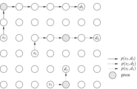
Figure 5 shows an example of S4. We consider the same example as for RSSS and CSSS (see Figure 3 and

Figure 4). Each source computes the distance to each sink by using pivot nodes as relay. s1 chooses d1as sink

and S4 stores the path p(s1, d1) in

P

s3 s2 s1 d3 d2 d1 p(s3, d3) p(s2, d2) p(s1, d1) pivot

Figure 5: S4 avoids congested zones by using pivots.

d2 is distant enough from p(s1, d1). S4 adds the nodes used by p(s2, d2) to

P

is not in use yet and checks if it can sends data to this sink by using nodes that are not stored in

P

distant enough from the other existing paths. S4 selects pivots yielding to paths that are distant enough in order to reduce interference between paths and congestion in the whole network. Paths between sources and sinks are not necessarily shortest paths, but they are distant (when it is possible).

5

Simulations

This section is divided into two parts. First, we compare the distance between paths computed by S4 with the distance between paths computed using our ILP and by RSSS and CSSS. This comparison is applied on small network topologies of 20 nodes (in order for the ILP to find optimal solutions in a reasonable time). Second, we compare the network performance of S4 with those of RSSS and CSSS on larger topologies.

5.1 Simulations on small topologies

Here, we compare S4 with three strategies: the ILP, RSSS and CSSS. Due to the time required by ILP to find

optimal solutions, we only consider small topology of 20 nodes randomly distributed on a 100×100 square

meters topology. The communication range is set to 30 m. Results are averaged over 100 repetitions.γis set to

one eleventh: the gap between paths (in terms of distance) is considered to be ten times more important than the total distance of the paths.

The metric used for comparison is the average distance between paths, defined in the following way. Each strategy produces a set of paths

P

is computed. The distance between two paths p1 and p2 is equal to the minimum distance between any nodes

x∈ p1 and y∈ p2. Then, the average distance between paths is the average of the distances of all the paths,

∑p∈PdP(p)/card(

P

P

P

node is common, d(p1, p2) = 0 and thus, dP(p1) = 0.

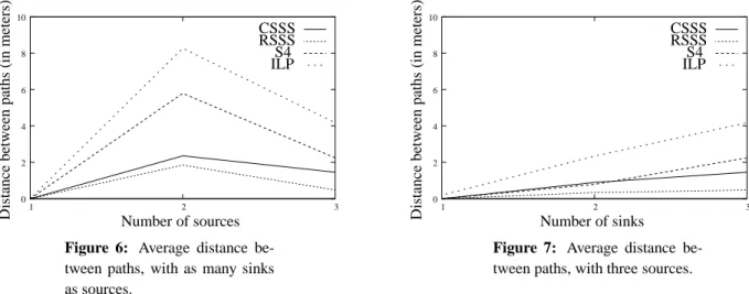
sinks as sources, for the four strategies. The distance is measured in meters. We notice that the maximum average distance is reached when there are two sources and two destinations. In this case, the average distance is 8 meters for ILP, 6 meters for S4, 2 meters for CSSS, and 1.8 meters for RSSS. For small network topologies, when the number of sources and sinks increases, the distance between paths decreases as the paths cannot be distant. We also notice that paths in S4 are only 25% less distant than in ILP. RSSS and CSSS both compute paths that are close to each other, and thus that yield congestion.

0 2 4 6 8 10 1 2 3 Number of sources D is ta n ce b et w ee n p at h s (i n m et er s) ILP RSSS CSSS S4

Figure 6: Average distance

be-tween paths, with as many sinks as sources. 0 2 4 6 8 10 1 2 3 Number of sinks D is ta n ce b et w ee n p at h s (i n m et er s) ILP RSSS CSSS S4

Figure 7: Average distance

be-tween paths, with three sources.

Figure 7 shows the average distance between paths as a function of the number of sinks, for the four strategies. The number of sources is constant and set to 3. We notice that the average distance increases with the number of sinks. This is due to the fact that by increasing the number of sinks, the possibilities of having distant paths increase. As expected, the ILP formulation shows the better performance. S4 is able to reach 75% of the performance of ILP. The maximum average distance is obtained when the number of sinks equals to the number of sources.

5.2 Simulations on large topologies

In this section, we describe the simulations we ran in order to compare S4 with RSSS and CSSS on larger topologies. We use version 2.31 of the NS-2 simulator. We use IEEE 802.15.4 physical and MAC layers with the non-beacon enabled mode. The propagation model is the probabilistic two ray ground model, with default parameters. The transmission power is set to a realistic value of -25 dBm, which yields a communication range of about 25 m. The size of the nodes queue is set to 50 packets.

In the simulations, we considered topologies of 100 nodes, randomly distributed on an area of 100×100

meter square. All sensors are full function devices with routing capabilities. The PAN coordinator is located at the center of the area. We wait for the network to be fully associated before injecting data packets. Data packets of 77 bytes (at the physical layer) are generated during 50 seconds, at a rate varying between 0.5, 1, and 2 packets

per source and per second. The routing protocol used for the three strategies is AODV2 _{(Perkins et al., 2003).}

Notice that before AODV can send packets to an unknown destination, it has to establish a path through reply and request messages, which introduces delay3. In order to have consistent results (especially for RSSS), results are averaged over 100 repetitions.

2_{AODV is slightly modified in S4 in order to allow pivot nodes}

3_{For RSSS and CSSS, AODV has to establish paths from each source to its assigned destination. For S4, AODV has to establish}

5.2.1 Performance metrics

Our mechanism is evaluated and compared to RSSS and CSSS according to the following performance met-rics: average distance (computed as in 5.1), packet loss (computed as the number of received packets over the number of generated packets), and end-to-end delay (defined as the time interval between a packet trans-mission and its reception by the sink). In the following, figures show the metric performances by considering 100 nodes randomly spread in the network. Similar results are obtained by considering grid networks of 49 nodes (El Rachkidy et al., 2010).

5.2.2 Average distance between paths

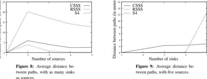
Figure 8 shows the average distance between paths for the three strategies, as a function of the number of sources, with a number of sinks equal to the number of sources. The average distance reaches a maximum for two sources: as the number of sources increases, more paths have to be computed, which decreases the average distance between paths. RSSS computes paths that often intersect, which rapidly decreases the average distance. S4 is able to build paths whose average distance is between 13 and 20 meters (with our settings), which limits interferences among paths, and thus improves overall performance.

0 5 10 15 20 25 1 2 3 4 5 Number of sources D is ta n ce b et w ee n p at h s (i n m et er s) RSSS CSSS S4

Figure 8: Average distance

be-tween paths, with as many sinks as sources. 0 2 4 6 8 10 12 14 16 1 2 3 4 5 Number of sinks D is ta n ce b et w ee n p at h s (i n m et er s) RSSS CSSS S4

Figure 9: Average distance

be-tween paths, with five sources.

Figure 9 shows the average distance between paths for the three strategies, as a function of the number of sinks, with five sources. None of the strategies are able to perform very well with these settings, as the number of sinks is smaller than the number of sources. The fact that CSSS is able to produce paths that have an average distance greater than zero means that, on average, one source (out of the five) was assigned to its own sink. While the distance for the four other paths might be zero, the distance between the fifth path (with its own sink) and the other paths is not zero, which makes the average distance not zero as well. S4 is only able to produce distant paths when the number of sinks is high enough, and in our case, when it is equal to the number of sources.

5.2.3 Packet loss

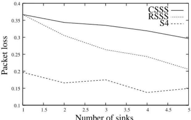
Figure 10 and Figure 11 show the average packet loss as a function of the number of sources and sinks, with a data rate equals to 2 packets per source and per second. We notice that the packet loss for the three strategies increases consistently with the number of sources, and decreases with the number of sinks. When the number of sources in the network is large, the traffic load is large too and the medium is overloaded by the generated packets. Also, paths cannot be as distant as when the number of sources is small. S4 is able to significantly reduce the

packet loss compared to RSSS and CSSS, especially when there are many sinks. Indeed, S4 aims to build distant paths by selecting pivots for each source-sink pair, which contributes to balance the traffic between nodes and to reduce congestion on the medium. When the number of sources and sinks is small, the use of pivots increases the length of paths, and S4 exhibits worse performance than RSSS and CSSS. However, for five sources and five sinks, S4 reduces by approximately 25% the packet loss probability of RSSS and 50% the packet loss probability of CSSS. S4 also outperforms the other two strategies when there are five sources and one sink: S4 reduces by approximately 46% the packet loss probability of RSSS and CSSS for five sources and one sink.

0 0.05 0.1 0.15 0.2 0.25 0.3 1 1.5 2 2.5 3 3.5 4 4.5 5 RSSS CSSS S4 P ac k et lo ss Number of sources

Figure 10: Packet loss rate, with

as many sinks as sources.

0.1 0.15 0.2 0.25 0.3 0.35 0.4 1 1.5 2 2.5 3 3.5 4 4.5 5 RSSS CSSS S4 P ac k et lo ss Number of sinks

Figure 11: Packet loss rate, with

five sources.

5.2.4 End-to-end delay

Figure 12 shows the average end-to-end delay for the three strategies, as a function of the number of sources, with a number of sinks equal to the number of sources and with a data rate equals to 2 packets per source and per second. The number of nodes used in the network is 100. For RSSS, the delay increases with the number of sources and sinks and becomes stable when there are more than four sources in the network. The delay is positively affected by the number of sinks (as the average distance between a source and a sink decreases) and negatively affected by the traffic load (as the medium becomes congested). Surprisingly, it can be noticed that CSSS induces larger delays than RSSS. This is explained by the fact that CSSS tends to select the same sink for several close sources, which yields to congested areas around these sinks. RSSS balances the sink usage by choosing sinks randomly. While CSSS and RSSS have almost the same packet loss (see Figure 10 and Figure 11), the impact on delay is significant: packets with large delay are more likely to be dropped in RSSS, which reduces the average packet loss for this strategy. S4 has the best behavior of the three strategies. This proves that it is important to consider the sink selection and the route establishment jointly. S4 reduces the average end-to-end delay over CSSS by 66% and over RSSS by 48%, for five sources and five sinks.

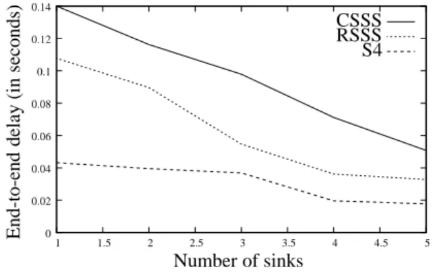
Figure 13 shows the average end-to-end delay for the three strategies, for five sources, as a function of the number of sinks. For the three strategies, we notice that the delay decreases with the number of sinks. With a large number of sinks, there are less congested areas in the network, and thus the number of packet retransmissions decreases (because the packet loss decreases too, see Figure 11). S4 outperforms the two other strategies, even with one sink: in this case, it reduces the end-to-end delay of CSSS and RSSS by 70%. This is achieved by choosing pivots that force the five paths to be distant (except at the sink where they meet), and thus reducing interferences among these paths.

0.005 0.01 0.015 0.02 0.025 0.03 0.035 0.04 0.045 0.05 0.055 0.06 1 1.5 2 2.5 3 3.5 4 4.5 5 RSSS CSSS S4 E n d -t o -e n d d el ay (i n se co n d s) Number of sources

Figure 12: End-to-end delay, with as many sinks as sources.

0 0.02 0.04 0.06 0.08 0.1 0.12 0.14 1 1.5 2 2.5 3 3.5 4 4.5 5 RSSS CSSS S4 E n d -t o -e n d d el ay (i n se co n d s) Number of sinks

Figure 13: End-to-end delay, with five sources.

5.3 Network performance with a varying data rate

In this subsection, we study the impact of the data rate on the network. We always consider a network of 100 nodes randomly deployed. We set the number of source as well as the number of sinks to three. Then, we study the behavior of the three strategies (CSSS, RSSS, and S4) in the network.

Figure 14 shows the average packet loss in terms of the data rate. The packet loss increases by increasing the traffic load in the network. We notice that S4 outperforms CSSS by 60% and RSSS by 33% for a data transmission rate of 2 packets per source and per second. We also notice that even with small data rate (0.5 packet per source and per second), S4 has the best behavior and shows a gain of 65% compared to CSSS and 50% compared to RSSS. Figure 15 shows the average end-to-end delay as a function of the data rate for the three strategies. As the data rate increases, the end-to-end delay decrease because the packet loss becomes higher and several packets are dropped. The packets most likely to be dropped are those that correspond to long routes. We also notice that S4 shows a gain of 74% (respectively 61%) compared to CSSS and 60% (respectively 59%) compared to RSSS for a data rate of 2 (respectively for a data rate equals to 0.5).

0.06 0.08 0.1 0.12 0.14 0.16 0.18 0.2 0.22 0.24 0.26 0.4 0.6 0.8 1 1.2 1.4 1.6 1.8 2 RSSS CSSS S4 P ac k et lo ss

Data rate (per source per second)

Figure 14: End-to-end delay, with three sources and three sinks. 0.01 0.015 0.02 0.025 0.03 0.035 0.04 0.045 0.05 0.055 0.06 0.065 0.4 0.6 0.8 1 1.2 1.4 1.6 1.8 2 RSSS CSSS S4 E n d -t o -e n d d el ay (i n se co n d s)

Data rate (per source per second)

Figure 15: End-to-end delay, with three sources and three sinks.

6

Distributed version of S4

In the centralized version of S4, we made the following assumptions. First, the entity that performs the compu-tation knows the whole topology, in order to compute the paths from any source to any destination via any pivot, or the hop counts. Second, sources were considered sequentially by a central entity. Third, the topology is static and nodes do not fail.

In the following, we describe how the centralized assumptions can be removed in order to make S4 a distributed protocol. The main requirements of the distributed version of S4 are the following. First, a local computation is performed by every source. Second, each source knows the set of all sinks. Note that no node is required to know the whole topology.

The hop count between two nodes can be computed using a simple signalling protocol, or using properties of hierarchical addresses (such as those used in ZigBee (ZigBee, 2008) for example). Similarly, the number of nodes in common between two paths can be computed by having s send a first message to x, and a second message via x to d. Each node on both paths can send a notification back to s, containing the path traveled. With this information, s is then able to count the number of common nodes. Another possibility is again to use properties of hierarchical addresses, which allows a node s to determine the path between two nodes a and b, provided that the addresses of a and b are known and that s has a knowledge of the network parameters (such as maximum number of child routers per node, maximum number of children per node, and maximum depth). We assume that hierarchical addresses are used, which avoids the use of additional control messages.

Sources advertise themselves to other neighbor sources, using a limited flooding protocol. Ignoring sources that are far away might be suboptimal when considering routes and sinks, but generally, it is better to avoid very long paths, even if they are distant to other paths. Once sources know their neighbor sources, they schedule their pivot and sink selection according to any order (which can depend on their address, for instance). Once a source has computed its own pivot and sink, it broadcasts this information to all neighbor sources. Then, the next sources in the order compute their own pivots and sinks, until all the sources have performed this task.

The determination of pivots by a source is achieved by using a limited flooding (common to each potential sink). The flooding is restricted to nodes that are close to the shortest path from the source to one of the sink. Indeed, it is not efficient to consider pivots that are too far away from the shortest path from the source to one sink.

To summarize, each source sends the three following messages in order to compute its pivot and sink. First, the source identifies neighbor sources by using a flooding limited to the region around the source. Second, the source identifies potential pivots by using a flooding limited to the nodes that are close to the shortest path from the source to one of the sink. Third, the source informs the neighbor sources of its selected pivot and sink by using a flooding, limited to the region around the source.

When the topology changes, the routing protocol upon which S4 is built detects the change and modifies the routes. Such changes can cause initially distant routes to become closer or even to overlap. Such overlaps can reduce the performance of S4. To avoid this problem, it is important for each source to recompute periodically the set of potential pivots. However, a trade-off has to be made between the control overhead caused by determining pivots, and the performance reduction caused by keeping inefficient pivots in case of topology changes.

Additionally, the failure of pivots has a negative impact on S4, as packets are routed to pivots before being routed to the sink. A pivot failure has to be reported to the source by the routing protocol (using notifications indicating a failure to deliver to the pivot) or by the sink (which stops receiving messages from the source). Upon receiving this report, the source can choose another pivot from the set of previously computed potential pivot. If this set is empty, the source has to initiate another pivot detection.

7

Conclusion

In this chapter, we showed that it is important to perform jointly sink selection and route computation in an anycast, multi-sink deployment. We showed that determining distant paths from sources to sinks is an NP-hard problem, and we proposed an integer linear program that computes optimal solutions, using the global knowledge of the topology and heavy processing power. Then, we proposed an heuristic called S4 based on realistic assumptions. S4 is an approach that selects sinks and pivots to provide distant paths between source-sink pairs, in order to reduce congestion in the network. Simulation results showed that S4 outperforms the existing strategies in terms of delay (which is reduced by up to 50% in our scenarios) and packet loss (which is reduced by up to 41% in our scenarios). S4 is also shown to produce paths that are on average distant from each other. We conclude this work by proposing a method to distribute S4, which requires a limited amount of control messages and a partial vision of the topology.

Acknowledgment: This work has been partially supported by a research grant from the Lebanese National

Council for Scientific Research (LNCSR).

References

Buratti, C., Orris, J., & Verdone, R. (2006). On the design of tree-based topologies for multi-sink wireless sensor nerworks.

Chang, J. & Tassiulas, L. (2007). Maximum lifetime routing in wireless sensor networks. IEEE/ACM Transac-tions on Networking, 12(4).

El Rachkidy, N., Guitton, A., & Misson, M. (2009). Pirat: Pivot routing for alarm transmission in wireless sensor networks. In IEEE Local Computer Networks.

El Rachkidy, N., Guitton, A., & Misson, M. (2010). Routing protocol for anycast communications in a wireless sensor network. In IFIP Networking, LNCS.

He, T., Krishnamurthy, S., Stankovic, J. A., Abdelzaher, T., Luo, L., Stoleru, R., Yan, T., Gu, L., Hui, J., & Krogh, B. (2004). Energy-efficient surveillance system using wireless sensor networks. In International Conference on Mobile Systems, Applications and Services (pp. 270–283).

Hu, W., Bulusu, N., & Jha, S. (2005). A communication paradigm for hybrid sensor/actuator networks. Springer International Jounal of Wireless Information Networks, 14(3).

Intanagonwiwat, C., Govindan, R., Estrin, D., Heidemann, J., & Silva, F. (2003). Direct diffusion for wireless sensor networking. IEEE/ACM Transactions on Networking (TON), 11, 2–16.

Juang, P., Oki, H., Wang, Y., Martonosi, M., Pen, L. S., & Rubenstein, D. (2002). Energy-efficient computing for wildlife tracking: design tradeoffs and early experiences with ZebraNet. ACM SIGOPS Operating Systems Review, 36(5), 96–107.

Kalantari, M. & Shayman, M. (2006). Design optimization of multi-sink sensor networks by analogy to electro-static theory. In IEEE WCNC.

Kim, H., Seok, Y., Choi, N., & Kwon, T. (2005). Optimal multi-sink positioning and energy-efficient routing in wireless sensor networks. In Information Networking.

Kim, J., Lin, X., & Shroff, N. B. (2008). Minimizing delay and maximizing lifetime for wireless sensor networks with anycast. In IEEE INFOCOM.

Lee, S. J. & Gerla, M. (2001). Split multipath routing with maximally disjoint paths in ad hoc networks. In IEEE ICC.

Luo, D., Zuo, D., & Yang, X. (2008). An optimal sink selection scheme for multi-sink wireless sensor networks. In Computer Science and Information Technology ICCSIT.

Marina, M. K. & Das, S. R. (2001). On-demand multipath distance vector routing in ad hoc networks. In ICNP. Oyman, E. I. & Ersoy, C. (2004). Multiple sink network design problem in largescale wireless sensor networks.

In IEEE ICC.

Pearlman, M. R., Haas, Z. J., Sholander, P., & Tabrizi, S. S. (2000). On the impact of alternate path routing for load balancing in mobile ad hoc networks. In ACM Mobile Ad Hoc Networking and Computing.

Perkins, C., Belding-Royer, E., & Das, S. (2003). Ad hoc On-Demand Distance Vector (AODV) Routing. Request For Comments 3561, IETF.

Qian-Ping, G., Satoshi, O., & Shietung, P. (1994). Efficient algorithms for node disjoint path problems. Proceed-ings of Electronics, Information and Communication Engineers Conference, 2.

Saha, D., Toy, S., Bondyopadhyay, S., Ueda, T., & Tanaka, S. (2003). An adaptive framework for multipath routing via maximally zone-disjoint shortest paths in ad hoc wireless networks with directional antenna. In Proc. Global Telecommunications.

Shukla, I. & Menghanathan, N. (2005). Impact of leader selection strategies on the PEGASIS data gathering protocol for wireless sensor networks. Ubiquitous Computing and Communication Journal.

Thepvilojanapong, N., Tobe, Y., & Sezaki, K. (2005). Har: Hierarchy-based anycast routing protocol for wireless sensor networks. In SAINT.

Wang, Z., Bulut, E., & Szymanski, B. K. (2009). Energy efficient collision aware multipath routing for wirelss sensor networks. In IEEE ICC.