Extreme events in extended nonlinear optical cavities

HAL Id: tel-01996688

https://tel.archives-ouvertes.fr/tel-01996688

HAL is a multi-disciplinary open access archive for the deposit and dissemination of sci-entific research documents, whether they are pub-lished or not. The documents may come from teaching and research institutions in France or abroad, or from public or private research centers.

L’archive ouverte pluridisciplinaire HAL, est destinée au dépôt et à la diffusion de documents scientifiques de niveau recherche, publiés ou non, émanant des établissements d’enseignement et de recherche français ou étrangers, des laboratoires publics ou privés.

Cristina Rimoldi

To cite this version:

Cristina Rimoldi. Extreme events in extended nonlinear optical cavities. Physics [physics]. COMUE Université Côte d’Azur (2015 - 2019), 2017. English. �NNT : 2017AZUR4095�. �tel-01996688�

I

P

N

THÈSE

pour obtenir le titre de

Docteur en Sciences

de l’Université Côte d’Azur Discipline

P

Événements extrêmes dans des cavités optiques

non linéaires étendues

Extreme events in extended nonlinear optical cavities

presentée et soutenue par

Cristina R

IMOLDI

dirigée par

Giovanna T

et Franco P

soutenue le 8 Décembre 2017 devant le jury composé de:

Pr. Gian-Luca OPPO - Rapporteur

Pr. Andrei VLADIMIROV - Rapporteur

Dr. Stephane BARLAND - Examinateur

Pr. Massimo GIUDICI - Examinateur

Pr. Abdelmajid TAKI - Examinateur

Pr. Franco PRATI - Codirecteur

I

P

N

THÈSE

pour obtenir le titre de

Docteur en Sciences

de l’Université Côte d’Azur Discipline

P

Événements extrêmes dans des cavités optiques

non linéaires étendues

Extreme events in extended nonlinear optical cavities

presentée et soutenue par

Cristina R

IMOLDI

dirigée par

Giovanna T

et Franco P

soutenue le 8 Décembre 2017 devant le jury composé de:

Pr. Gian-Luca OPPO - Rapporteur

Pr. Andrei VLADIMIROV - Rapporteur

Dr. Stephane BARLAND - Examinateur

Pr. Massimo GIUDICI - Examinateur

Pr. Abdelmajid TAKI - Examinateur

Pr. Franco PRATI - Codirecteur

1.3 HSSs and linear stability analysis . . . 27

1.3.1 Bistability . . . 29

1.3.2 Plane-wave instability . . . 30

1.3.3 Pattern-forming instabilities. . . 32

1.4 Zoology of the stationary and nonstationary solutions . . . 33

1.4.1 Cavity solitons . . . 34

1.4.2 Extended spatiotemporal chaos. . . 35

1.4.3 Chaotic cavity solitons . . . 38

1.4.4 Oscillatory cavity solitons . . . 40

1.4.5 Role of the diffusion coefficient d . . . 42

1.5 Extreme event detection . . . 43

1.5.1 Maxima individuation method . . . 43

1.6 Statistical analysis . . . 45

1.6.1 PDF of the spatiotemporal maxima. . . 45

1.6.2 Rayleigh and negative exponential PDF . . . 48

1.6.3 Weibull PDF . . . 50

1.6.4 Gumbel PDF . . . 51

1.7 Dependence on the laser parameters . . . 53

1.8 Comparison with other works in the field . . . 57

1.9 Waiting time statistics . . . 60

1.10 Profiles and cavity soliton comparison . . . 61

1.11 Future perspectives . . . 64

1.11.1 Conservative limit of a LSA . . . 64

1.12 Conclusions . . . 68

2 Semiconductor ring laser with injection 69 2.1 Introduction . . . 70

2.2 Model . . . 71

2.2.1 Low transmission limit. . . 74

2.2.2 Rate-equation model . . . 75

2.2.3 Rate-equation model with a term of diffusion. . . 76

2.2.4 Modified forced Ginzburg-Landau model. . . 76

2.2.5 Rate-equation model with a Ginzburg-Landau term . . . . 80

2.3 HSS and linear stability analysis . . . 81

2.3.1 Comparison of the different models . . . 83

2.4 Experimental setup . . . 88

2.5 Phase solitons and complexes . . . 89

2.5.1 Parameter choice . . . 91

2.5.2 Single-charge phase soliton . . . 92

2.5.3 Attractive interaction. . . 96

2.5.4 Multiple-charge phase solitons . . . 100

2.6 Extreme events from phase soliton collisions . . . 103

2.6.1 Experimental results . . . 103

2.6.2 Numerical simulations . . . 105

2.7 High-peak events in unstable roll regime . . . 108

2.7.1 Roll patterns . . . 108

2.7.2 Spectral analysis . . . 112

2.7.3 High-peak events and statistical analysis . . . 112

2.7.4 Phase dynamics . . . 115

2.8 Conclusions . . . 125

3 Broad-area semiconductor laser with injection 127 3.1 Introduction . . . 127

3.2 Model. . . 128

3.3 HSS and linear stability analysis . . . 129

3.4 CS interaction . . . 133

3.4.1 Interaction potential and merging time . . . 136

3.4.2 Possible analogy with hydrophobic materials. . . 139

3.5 Extreme event investigation . . . 140

3.6 Conclusions . . . 145

Conclusions 147

Appendices 151

A LSA equations in physical variables 151

B Split-step method for Eqs.(1.1) 153

C The Routh-Hurwitz stability criterion 155

D Log-Poissonian distribution 157

E LSA conservative limit 161

F Split-step method for Eqs.(2.7), (2.8) 167

G Split-step method for Eqs.(3.2) 169

List of acronyms 173

Bibliography 175

1.1 Example of a VCSEL with intracavity SA . . . 24

1.2 Scheme of the LSA system . . . 26

1.3 HSSs and ωsfor LSA . . . 27

1.4 Stationary and Hopf instability domains . . . 33

1.5 HSSs and other solutions for the LSA. . . 34

1.6 Stationary CS in the intensity transverse plane and its Fourier op-tical spectrum . . . 35

1.7 Extended spatiotemporal chaos in the intensity transverse plane and its phase . . . 36

1.8 Fourier optical spectrum for the extended spatiotemporal chaos both in linear and logarithmic scale . . . 36

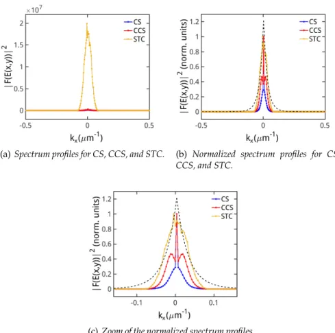
1.9 Fourier spectrum profiles for CS, CCS and STC . . . 37

1.10 CCS in the intensity transverse plane and its Fourier optical spec-trum. . . 38

1.11 Phase of the electric field for the CCS . . . 39

1.12 OCS in the intensity transverse plane and its Fourier optical spec-trum. . . 40

1.13 Fourier spectrum profile and time trace for a OCS and plot of the pulsation period as function of µ . . . 41

1.14 Fourier spectrum for different values of diffusion coefficient . . . 42

1.15 Spatiotemporal maxima selection . . . 44

1.16 3D spatiotemporal grid representation . . . 44

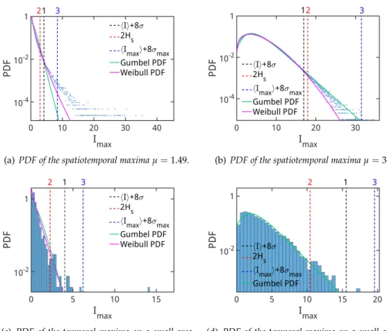
1.17 PDFs of the spatiotemporal maxima . . . 46

1.18 PDFs of the total intensity . . . 48

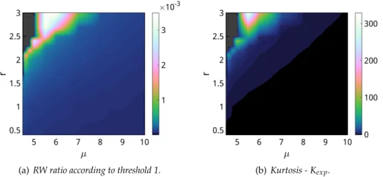
1.19 Density plots of RW ratio and kurtosis for the PDFs of spatiotem-poral maxima . . . 54

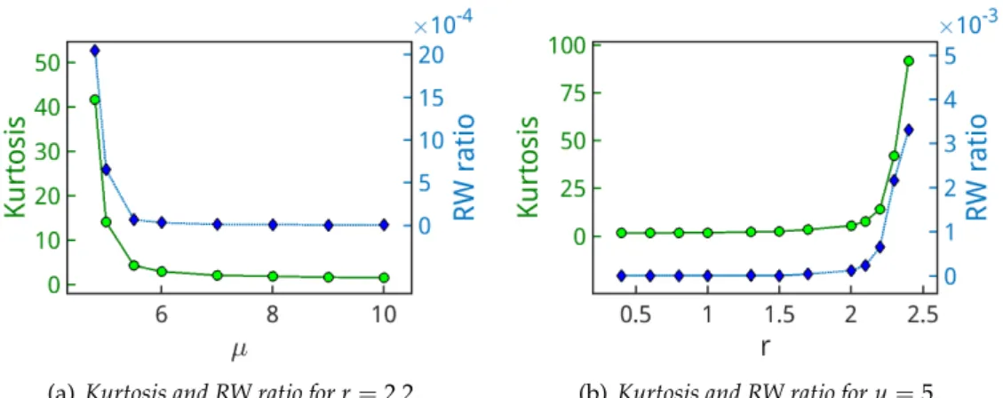
1.20 Density plots of RW ratio and kurtosis for the PDFs of total intensity 55 1.21 Time trace of the spatially averaged intensity for µ=5 and r=2.4 56 1.22 Kurtosis and RW ratio for fixed r and µ . . . 56

1.23 HSSs and extended spatiotemporal chaos branch for different pa-rameters . . . 57

1.24 Kurtosis and RW ratio for fixed r for different parameters . . . 58

1.25 Results from [Selmi 2016] . . . 59

1.26 Time trace of the intensity averaged on a small area . . . 59

1.27 PDFs of the spatiotemporal maxima and of the temporal maxima of a time trace spatially averaged on a small area . . . 60

1.28 PDF of the logarithmic waiting times between two consecutive extreme events. . . 61

1.29 Extreme event in the intensity transverse plane and PDFs of spa-tiotemporal maxima and total intensity . . . 62

1.30 Temporal and spatial profiles for I, D and ¯D of the extreme event in Fig. 1.29 . . . 62

1.31 Comparison between the spatial and temporal profiles of cavity solitons and extreme events . . . 63

1.32 Toda potential . . . 67

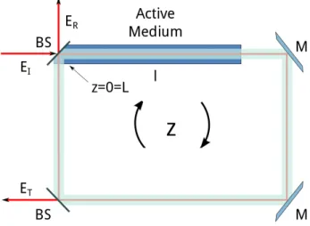
2.1 Scheme of a ring laser with optical injection . . . 70

2.2 Scheme of the ring laser used in the model derivation . . . 71

2.3 HSS and bistability boundaries for the ring laser with injection. . 81

2.4 Instability domains for models in Eqs. (2.5), (2.7) and (2.8) . . . . 84

2.5 HSS for the ring laser with injection with highlighted three fixed points for a given value of injection . . . 84

2.6 HSS and instability boundaries for specific choices of parameters 86 2.7 Instability domains for the models in Eqs. (2.7), (2.5) and (2.8) for d=10−12 _{. . . . 86}

2.8 HSSs for specific choices of parameters. . . 87

2.9 Instability domains for the parameter choices in Fig. 2.8 . . . 87

2.10 Ring laser experimental setup . . . 88

2.11 Fabry-Perot experimental setup . . . 89

2.12 Spatiotemporal diagrams in the experimental and numerical ref-erence frame . . . 90

2.13 HSS and PS branch . . . 92

2.14 PSs at the boundaries of the stability domain . . . 93

2.15 PS phase space. . . 94

2.16 Experimental PS . . . 95

2.17 PS velocity and width . . . 96

2.18 Attractive interaction between PS as seen in the experiment . . . 96

2.19 Attractive interaction between PS of single and multiple charges . 97 2.20 Attractive interaction between PS of single and multiple charges in two special cases . . . 97

2.21 Interaction between single-charge PSs . . . 98

2.22 Single-charge PSs merging time as function of the initial distance 99 2.23 Multiple charge PSs . . . 99

2.24 Multiple charge PS as seen in the experiment . . . 100

2.25 Velocity as function of the PS chiral charge . . . 100

2.26 Double-charge PS as seen in the experiment . . . 100

2.27 Double and triple charge PSs as seen in the experiment . . . 101

2.28 Double and triple charge PSs in the phase space . . . 103

2.29 Collisional regime as seen in the experiment . . . 104

2.30 Experimental PDF of the intensity for the collisional regime . . . 105

2.31 Collisional regime as observed in the simulation . . . 106

2.40 PDFs of the peak height and total intensity . . . 115 2.41 Experimental histogram of the peak heights and PDF of the total

intensity . . . 115 2.42 Spatiotemporal diagram and PDF of peak height for different

val-ues of detuning . . . 116 2.43 Time trace of the carrier density and its adiabatic value . . . 117 2.44 Experimental and numerical histograms for the electric field in

the complex plane . . . 118 2.45 Experimental phase time trace. . . 120 2.46 Spatiotemporal diagram and temporal profiles around an

abnor-mal event as seen in the experiment . . . 120 2.47 Experimental phase portraits when approaching an abnormal event120 2.48 Numerical phase time trace . . . 121 2.49 Spatiotemporal diagram and phase time trace with highlighted 5

abnormal events . . . 121 2.50 Phase portrait in the(Re(E),Im(E))and(D, I)plane around an

abnormal event . . . 122 2.51 Spatiotemporal diagram for intensity and carrier density around

an abnormal event . . . 124 3.1 HSS for the semiconductor laser with optical injection. . . 129 3.2 Stationary instability domain of the model in Eqs. (3.2) for a

spe-cific choice of parameters. . . 131 3.3 Hopf instability domains of the model in Eqs. (3.2) for specific

choices of parameters. . . 131 3.4 Stationary and Hopf instability domains of the model in Eqs. (3.3)

for a specific choices of parameters.. . . 133 3.5 CSs merging process for σ=400 and d0=10 spatial units. . . 134 3.6 Time evolution of cavity soliton distances for different initial

val-ues and σ=400.. . . 135 3.7 Merging time of two CSs as a function of their initial distance. . . 136 3.8 Temporal evolution of the distance between two CSs for σ = 400

and r0=10. . . 137 3.9 CSs merging time as a function of their initial distance for

differ-ent values of σ. . . . 138 3.10 CSs merging time as a function of 1/σ for different initial distances.139 3.11 Example of the chaotic regime observed for low values of optical

injection. . . 141 3.12 PDFs of total intensity and spatiotemporal maxima. . . 142 3.13 Example of extreme event in the electric field intensity. . . 143

3.14 Color maps of the electric field intensity, the phase of the electric field and the carrier density in presence of an extreme event. . . . 143 3.15 System trajectory in the (D, φ, I) phase space in the spot of the

extreme event. . . 144 3.16 Phase and zero isolines of the real and imaginary part of the

elec-tric field around the extreme event. . . 144 E.1 Relaxation oscillations in a class B laser and comparison between

the numerically integrated and theoretical periods T1and T2 . . . 164 E.2 Comparison between the predicted periods and the data

freedom, either in the transverse plane, perpendicular to the direction of propa-gation of light, or in the propapropa-gation direction. Localized structures of different nature represent an important possible solution in each one of the systems here studied, hence their interaction and the role played in the formation of extreme events have been also investigated into details.

In the first system, a monolithic broad-area semiconductor laser (VCSEL) with an intracavity saturable absorber, we report on the occurrence of extreme events in the 2D transverse plane of the electric field intensity. In particular we high-light the connection between these objects and cavity solitons, both stationary and oscillatory, also present in the system.

In the second system, a highly multimode laser with optical injection spatially extended along the propagation direction, we analyze the interaction and merg-ing of phase solitons, localized structures propagatmerg-ing along the cavity carrymerg-ing a 2π phase rotation. Extreme events have been investigated in two configura-tions: a first one where they emerge from the collision of phase solitons with other transient structures carrying a negative chiral charge, and a second one where high-peak events emerge from an unstable roll regime where phase soli-tons are not a stable solution. In both these systems we investigate the role of chirality in the extreme event formation.

In the third system, a broad-area semiconductor laser (VCSEL) with optical in-jection, we study into details the interaction of cavity solitons in the transverse plane, described as two particles subjected to an interaction potential exponen-tially decreasing with the distance between the two objects: a possible analogy with hydrophobic materials is here suggested. Some preliminary results show-ing spatiotemporal extreme events in this system are also given.

KEYWORDS: dynamics of nonlinear optical systems – semiconductor lasers – extreme events – rogue waves – dissipative solitons.

ou deux degrés spatiales de liberté, soit dans le plan transversal (perpendicu-laire à la direction de propagation de la lumière) soit dans la direction de pro-pagation. Des structures localisées de nature différente constituent une solution possible importante dans chacun des systèmes étudiés ; leurs interaction autant que leurs rôle dans la formation des événements extrêmes ont donc été analysés en détails.

Dans le premier système, un laser à semiconducteur monolithique (VCSEL) à large surface avec un absorbant saturable, on présente la formation d’événe-ments extrêmes dans le plan transversal à deux dimensions de l’intensité du champ électrique. En particulier, on met en évidence la liaison entre ces objets et les solitons de cavité, soit stationaires soit oscillatoires, aussi présents dans le système.

Dans le deuxième système, un laser multimodal spatialement étendu dans la direction de propagation avec injection optique, on analyse l’interaction et la fusion des solitons de phase, des structures localisées qui se propagent dans la cavité en transportant une rotation de phase de 2π. Les événements extrêmes ont été étudié dans deux configurations : une première où ils émergent de la col-lision des solitons de phase avec des autres structures transitoires transportant une charge chirale négative, et une deuxième où des événements d’intensité éle-vée émergent d’un régime instable de motif en rouleau où les solitons de cavité ne sont pas des solutions stables. Dans les deux systèmes, on examine le rôle de la chiralité dans la formation des événements extrêmes.

Dans le troisième système, un laser à semiconducteur avec injection optique, on étudie dans les détails l’interaction des solitons de cavité dans le plan transver-sal, décrits comme deux particules soumises à un potentiel d’interaction décrois-sant exponentiellement avec la distance entre les deux objets : une analogie pos-sible avec les matériaux hydrophobes a été proposée. Des résultats préliminaires présentant des événements extrêmes spatiotemporels dans ce système sont aussi donnés.

MOTS-CLÉS : Dynamique des systèmes non linéaires – lasers à semiconduc-teur – événements extrêmes – vagues scélérates – solitons dissipatifs.

such as fibers, the playground has significantly broaden to include a multitude of different areas. In particular lasers are found to be an interesting workbench for the study of these phenomena, since they could allow us to shed some light on the deterministic nature of the extreme events observed and, in the case of extended cavities, to investigate the role of spatial effects.

The aim of this introduction is to place the topic of this Thesis in the context of extreme events, a subject of study in many different fields (i.e. society, econ-omy, geology, weather forecast and so forth). Then we will illustrate the main results that prompted the field in the optical context and focus on its broadening to nonlinear active dissipative systems. Finally we will discuss the role of local-ized structures and their interaction in this framework and illustrate the content of the present manuscript.

Extreme events in different fields

There are many phenomena that fall or could fall under the definition of extreme events, depending on the point of view of a person [Jentsch 2006]. For instance an event is usually considered extreme according to its rarity and catastrophic nature but these can be subjective concepts, for instance to an insurance com-pany an event is to be considered rare if it presents a low probability of occur-rence and catastrophic if it implicates big consequences. Hence, in this case, the extremeness of an event is considered in terms of both its impact and its fre-quency. To a scientist instead the main charm regarding extreme events consists in their uniqueness, and in the concept of whether or not it is actually possible to predict these objects. An event is considered extreme if it involves a big de-viation from a series of measurement [Jentsch 2006]. In this view for example a magnetic storm or a particularly violent earthquake can be considered as ex-treme events even if they do not, respectively, affect any device or occur in a inhabited area.

Extreme events in nature and society can affect a single individual, for ex-ample the contraction of a rare disease, as well as multiple people or the

(a) Hurricane Hugo in 1989 (b) Crowd gathering on Wall Street after the 1929 crash

Fig. 1 – Examples of extreme events in nature and society. (a) Hurricane Hugo occurring in 1989. Photo by NOAA / Satellite and Information Service, from Wikimedia Com-mons - Public Domain. (b) Crowd gathering on Wall Street after the 1929 Wall Street Crash which many believe lead to the following 12-year Great Depression affecting all Western industrialized countries. Photo from Wikimedia Commons - Public Domain.

vironment, for example natural disasters, such as floods or hurricanes, societal disasters, such as pandemics, or market crashes.

Given the variety of possible phenomena to be considered as extreme the most obvious approach for their characterization consists in the study of their statis-tics and dynamics, focusing in particular on the possible analogies between dif-ferent extreme events, their generating mechanisms and thus their predictability.

In general extreme events occur in the tail of a probability distribution. In many, but not all, cases [Jentsch 2006] the tails of a distribution containing ex-treme events are heavy, or subexponential, with exponential tails characterizing any Gaussian distribution. Given the probability distribution of an event it is possible to evaluate their probability of occurrence or even the probability of having any event larger than a certain threshold.

Some statistical theories have been developed on this topic [Gumbel 1958], but their working assumptions for the events to be independent and identically dis-tributed are very strong and rarely in good agreement with reality.

The other main approach in the study of extreme events consists in looking at the dynamical properties of the phenomenon. All extreme events in nature are usually expression of the complex dynamics of a system [Jentsch 2006]: they do not occur randomly but due to a dynamical mechanism that introduces huge excursions in the system trajectory, bringing it far from its normal state. Some examples of possible extreme events scenarios are those leading to deterministic chaos or turbulence [Jentsch 2006].

Even if no universal theory can be developed for extreme events, we may expect some similarities between different phenomena. We also would like to point out that these similarities can be both in the cause, i.e. the generating mechanism or the initial conditions, or in the effects. Similarities between

dif-[Jentsch 2006]. Nevertheless we have to remind that also in deterministic sys-tems chaos can emerge, causing the impossibility of long-term predictions [Erk-intalo 2015] even if this does not imply, on a short scale, the total lack of possible precursors.

Fiber optics and the analogy with hydrodynamics

A particular kind of extreme events, often studied in optics are rogue waves (RWs) which are also studied in oceanography and can be compared with this field, due to the well-known analogy between optics and hydrodynamics. Rogue waves are isolated high-amplitude waves occurring more frequently than ex-pected from Gaussian statistics [Kharif 2009,Onorato 2013].

The concept of rogue waves has been infamously well-known in oceanogra-phy since centuries, initially as anecdote or sailors’ tale and then, after the first experimental observations, like the Drapner wave in 1995 (see for example [Ha-ver 2000,Kharif 2009]), as an actual topic of study. In oceanography these objects are also called monster or freak waves and are known to destructively dam-age ships. There are different definitions for RWs, the main ones defining them as waves whose trough-to-crest height exceeds either two times the significant wave height (i.e. the mean of the highest third of the wave heights detected), or the mean plus eight times the standard deviation of the data. More details on the derivation of these definitions and rogue waves statistics are given in Chap-ter1.

Experimental measurements of rogue waves in oceanography present some difficulties [Onorato 2013]. The most used instrumentation consist in a buoy, registering the surface elevation data in a single point of the sea. Some evolu-tions of this technique include the possibility of collecting also the direction in-formation through the use of a directional buoy (see for example [De Pinho 2004]) and an alternative detection method consists in the use of a wave radar [Wy-att 2009]. In any case this kind of single point measurement presents some is-sues, since a simple temporal trace is not able to fully describe the spatiotempo-ral complexity of the sea surface. Since, to get a physical understanding of RW formation, some kind of space-time measurement is required [Onorato 2013], some alternative techniques have been proposed, among which the use of syn-thetic aperture radars (SARs) [Schulz-Stellenfleth 2004], but are still regarded with skepticism by the community [Janssen 2006]. More details on the experi-mental evidence of rogue waves in the ocean can be found in [Kharif 2009,

Ono-Fig. 2 – Reprinted with permission from [Solli 2007]. Schematization of the experimen-tal setup used by Solli et al. for the first reported experimenexperimen-tal observation of rogue waves in fibers.

rato 2013].

To understand the analogy drawn between optics and hydrodynamics re-garding rogue waves we have to consider the one dimensional nonlinear Schroe-dinger equation (NLSE)

i∂A ∂z +c1 ∂2A ∂t2 +c2|A| 2 A=0 .

In particular in hydrodynamics [Osborne 2010], with

c1 = −

k0

ω2₀ , c2

= −k3₀,

where k0is the wave number and ω0is the carrier frequency, the NLSE describes

the evolution of the surface wave group envelope in deep water. In fiber optics [Agrawal 2013], with

c1 = |β2|2

2 , c2= γ,

where β2 < 0 is the group velocity dispersion and γ the nonlinear coefficient,

the NLSE describes the evolution of a light pulse envelope propagating inside a fiber. Note that usually the NLSE in hydrodynamics has time and space switched, but this poses no peculiar obstacle to the analogy, except the fact that the coeffi-cients c1and c2need to be adapted [Osborne 2010,Dudley 2014].

From an historical point of view [Randoux 2016b] the discovery of multi-solitons as solutions of the NLSE [Zakharov 1972] prompted the optical field to the study of new solutions of the NLSE and eventually lead to the discovery of a new class of objects, describing the instability of a finite coherent background: these solutions are usually known as breathers, and include the Akhmediev breather [Akhmediev 1985] and the Peregrine soliton [Peregrine 1983], that is the Akhmediev breather limiting case for a period going to infinity [Kibler 2010]. These two solutions, in particular, fully describe the modulational instability process and were then suggested as rogue wave prototypes in oceanography [Dysthe 1999].

[Solli 2007].

With the seminal paper by Solli [Solli 2007] the concept of rogue waves started to be extended also to the optical context and the experimental obser-vation of breather solutions in both water wave tanks [Chabchoub 2011] and fibers [Kibler 2010,Frisquet 2013] brought forward the NLSE analogy in a rigor-ous way.

In the work by Solli, using the setup schematized in Fig. 2, the authors in-ject a mode-locked ytterbium-doped fiber laser into a nonlinear fiber generating supercontinuum: rogue waves where found in the heights of the electric field intensity at the output of the fiber, collected through the use of a photodetec-tor, after a filtering and signal enlargement process. A statistical analysis of the pulse heights showed L-shaped histograms largely deviating from the distribu-tion of most stochastic processes [Solli 2007] as illustrated in Fig.3.

This pioneering paper has the merit of introducing the concept of rogue waves to the optical community. Ever since the field has notably broadened and spe-cialized. In particular, regarding rogue waves in fibers, detection without the use of signal filters, has become more precise, allowing for a single-shot, real-time measurements [Suret 2016,Närhi 2016] in propagation.

Among other works in the fiber supercontinuum context we mention [Erk-intalo 2009,Kibler 2009,Mussot 2009]. Rogue waves have also been studied in the case of optical fiber propagation with [Taki 2010,Conforti 2015] and without [Walczak 2015] higher order dispersion, in the case of laser filamentation [Kas-parian 2009], passive cavities [Conforti 2015] and photorefractive ferroelectrics [Pierangeli 2015]. In the context of fibers but in case of an active system we mention RW study in Raman fiber amplifiers [Hammani 2008] and mode-locked fiber lasers [Zaviyalov 2012]. For a full review on the study of rogue waves and extreme events in different optical contexts please refer to [Onorato 2013, Dud-ley 2014,Akhmediev 2016].

The two most common generating mechanisms for rogue waves in fiber are modulational instability [Mussot 2009,Dudley 2009] and soliton or breather oc-currence [Akhmediev 2009,Kibler 2010,Kedziora 2013].

Rogue wave predictability has been investigated as well, in the systems de-scribed by the NLSE, both in oceanography [Latifah 2012, Alam 2014] and in optics [Akhmediev 2011a,Akhmediev 2011b,Birkholz 2015].

In the optical context in particular, Refs. [Akhmediev 2011a,Akhmediev 2011b] identify as an early warning for rogue wave occurrence, the emergence of a triangular shape (in logarithmic scale) in the spectrum related to the forma-tion of the Peregrine soliton and other higher-order soluforma-tions of the NLSE. In Ref. [Birkholz 2015] the authors use a novel approach, applying nonlinear time series analysis to search for traces of predictability directly in the experimen-tal data. Through the use of an adapted version of the method proposed by Grassberger and Procaccia [Grassberger 1983], the authors are able to distin-guish stochastic processes from processes where determinism prevails, making possible a prediction. In particular the method is based on dividing the time series in a sequence of smaller segments and computing the distances between the points of different segments: an elevated number of small distances implies similarities between different segments and can be interpreted as a signature of determinism, while in the stochastic case most distances will show large differ-ences between different segments. The authors search for similarities close to RW occurrence and identify multifilamentation as a mainly deterministic pro-cess where rogue waves appear with a warning. The application of the same method to the experimental data of the Draupner wave and to the power fluc-tuation data in the tail of the supercontinuum generation by Solli [Solli 2007] does not lead to the same conclusions but some issues are to be addressed [Erk-intalo 2015].

In general we can observe that, within the scientific community two parallel ways of exploring the analogy between optics and hydrodynamics have been outlined.

The first method focuses on the shape of the possible rogue waves: this ap-proach bases itself on the powerful possibility of finding the exact solutions of the NLSE and has fundamental historical reasons. As a general reminder we would like to point out that the NLSE in hydrodynamics, and also in optics, does not describe the shape of individual waves but their envelope, hence all the spe-cific envelope solutions of the NLSE, among which breathers and solitons, are not, in general, to be considered as individual rogue waves [Dudley 2014]. In recent works it has been observed that the shape of rogue waves, even in sys-tem configurations well described by the NLSE, might differ significantly from the well-known breather and Peregrine soliton solutions [Randoux 2016a]. Fur-thermore these specific solutions are generated in optical systems under very specific initial conditions, which result unlikely to be observed in the ocean [Randoux 2016b].

The second approach consists instead in finding similarities between the two fields from a statistical point of view [Onorato 2004, Erkintalo 2010]. In fact as we will illustrate more into details in Chapter1, under the assumption of a Gaussian distribution for the sea surface elevation it can be demonstrated that the amplitude of the water wave envelope (and with good approximation its height) would follow a Rayleigh distribution. In optics the main quantity un-der analysis is the intensity of the electric field and it can be demonstrated that, assuming a Gaussian distribution for the amplitude of the real and imaginary part of the electric field envelope, a negative exponential distribution for the in-tensity of the electric field envelope is to be expected. Hence if in oceanography

exploit its potential it is nevertheless necessary to treat such analogy within its limit. Since the NLSE has been reported as not able to describe ocean waves on short scales [Dyachenko 2005] we might expect other models, other than the NLSE, or an analogy on a statistical level to give us some additional insight on this topic. Furthermore a statistical approach could also help establish a link with the wider theory of extreme events in physics [Dudley 2014].

Extreme events in active optical systems

In the previous Section we have illustrated the development of the extreme event field in the context of fibers and some other optical systems. Most of the work on fibers is developed in conservative (or weakly dissipative) systems with propagative geometry. Lasers on the other hand are active, dissipative systems with possibly spatial degrees of freedom. Extreme events in this context have been observed in the configurations of optically injected [Bonatto 2011], mode-locked [Kovalsky 2011,Zaviyalov 2012,Lecaplain 2012], Raman [Randoux 2012] and pump-modulated [Pisarchik 2011] lasers.

The study of extreme events in (active) nonlinear optical cavities presents usually a different focus with respect to the fiber case. First of all, in the laser case, the main approach used in the investigation of extreme events is statistical, since none of the systems here presented are describable through the use of the one-dimensional nonlinear Schroedinger equation. Far from being a obstacle, this issue offers us the opportunity to reconnect to extreme event theory and even to the concept of rogue waves from a statistical perspective, exploring the analogy between the two field on a different level.

Most of research interest in this field is gathered around the investigation of the general physical or dynamical mechanisms at the base of extreme event forma-tion. In particular in the case of lasers these mechanisms include spatiotem-poral chaos [Selmi 2016], vortex turbulence [Gibson 2016], external crisis [Bon-atto 2011,Zamora-Munt 2013], dissipative solitons [Rimoldi 2017b] and soliton interaction [Walczak 2017].

The broadening of the extreme event field to the context of lasers allowed to study the deterministic nature of RWs and the consequences of the spatial ef-fect [Bonazzola 2013], an issue very relevant also in light of the analogy with oceanography.

Fig. 4 – Reprinted with permission from [Liu 2015]. Rogue wave formation in the spatial distribution of the electromagnetic energy. The color bar values are rescaled on the significant wave height of the field intensity. The white circle highlights the ultrafast, subwavelength rogue wave triggered by spontaneous synchronization.

more relevant to this Thesis.

In particular, regarding the subject of lasers with saturable absorber (LSA), we would like to mention the main results of [Bonazzola 2013, Selmi 2016, Couli-baly 2017].

In [Bonazzola 2013] the authors study the importance of spatial effects in the description of an all-solid-state LSA. In particular, using a rate-equation model with one equation for the electric field intensity, three equations for the pop-ulations in the laser levels and in the ground state and one equation for the difference of population in the saturable absorber, the authors analyze numer-ically different regimes, among which self-Q-switching, period doubling and deterministic chaos, well described by the model. Extreme events have been ob-served experimentally in some of the chaotic regimes for this type of laser [Ko-valsky 2011,Hnilo 2011] but have no matching numerical description with the rate-equation model, leading to the conclusion that spatial effects, not included in the model, actually play an essential role in the formation of extreme events for this kind of laser.

A few years later, in [Selmi 2016, Coulibaly 2017], the presence of extreme events is investigated experimentally and numerically in the transverse sec-tion of a semiconductor laser with an intracavity saturable absorber in a con-figuration of spatiotemporal chaos. The model there used to describe the laser [Bache 2005] includes spatial coupling through a diffractive term in the second derivative of the spatial coordinate in the equation for the electric field. Limiting their analysis to a single transverse spatial dimension, the authors observe the presence of extreme events in the experiment and in the simulations for certain choices of parameters. The origin of the observed extreme events is identified in spatiotemporal chaos, characterized through the Lyapunov coefficient anal-ysis and the Kaplan-Yorke dimension: in particular [Selmi 2016] a growth in the percentage of the observed extreme events is associated to an increase of the Kaplan-Yorke dimension. As a general reminder we would like to stress that, while a certain degree of spatiotemporal complexity might be considered a requirement for the observation of extreme events in this kind of system,

de-Fig. 5 – Reprinted with permission from [Zamora-Munt 2013]. System dynamics in the phase space when approaching and extreme event. S1, S2, S3 are three fixed points of the system, in particular S1 is a saddle, S2 and S3 are unstable foci. In (a) the blue dotted and green solid lines indicate, respectively, the stable and unstable manifolds of S2. (b) illustrates the system trajectory (highlighted in red) when approaching an extreme event, zoomed in (c). (d) Shows the intensity time trace.

terministic chaos is in general, at least experimentally, not a sufficient condi-tion [Kovalsky 2011].

More details on the results of these two articles in comparison with the results shown in this Thesis will be given in Chapter1.

In the context of lasers with optical injection we are going to focus on the study of systems with a different number of spatial dimensions [Bonatto 2011, Zamora-Munt 2013,Gibson 2016]. This will help us understand better if indeed spatial dimensionality affects the generating mechanisms of extreme events. Fur-thermore works in purely temporal (or with a very small transverse section) sys-tems confirm that space is actually not a requirement for the observation of ex-treme events, allowing for a simpler study of predictability and the role of noise.

The role of spatial dimensionality has been also investigated in other opti-cal context for example in cavities with liquid-crystal light valve as gain media [Montina 2009] and in the passive case, in photorefractive media [Pierangeli 2015] and photonic crystals [Liu 2015]. In particular in [Montina 2009] the nonlocal coupling between different spatial regions of the electric field intensity gives rise to symmetry breaking in the system and the presence of extreme events and in [Pierangeli 2015] the combination of disorder and nonlinearity appears to lead to extreme events observation. In [Liu 2015] extreme events are triggered in a photonic crystal through the control of a spontaneous synchronization mech-anism that enlarges the frequency bandwidth leading to high-peak pulses. A picture of rogue wave formation in the spatial distribution of the electromag-netic energy is illustrated in Fig.4.

In [Bonatto 2011,Zamora-Munt 2013] the authors study the setup of a single-transverse mode optically injected semiconductor laser (in particular a VCSEL). Given the very small laser transverse section, it is possible to describe the setup

as a zero-spatial dimension, purely temporal system. Extreme events are exper-imentally obtained when the slave laser emission frequency is unlocked from the frequency of the master laser and passes to a chaotic regime through period doubling. Note that extreme events are here observed at the beginning of the chaotic region but, since for more chaotic parameter choices the probability of large excursions in intensity increases, the extreme events threshold moves to-wards higher values of intensity displaying less extreme events in the system. The experimental results appear in good agreement with the numerical ones, achieved with a class-B rate-equation model for a semiconductor laser. Since ex-treme events do not appear every time the system is in a chaotic regime but in a very specific region of the phase space, the authors investigate the properties of the chaotic regions needed for the occurrence of extreme events. As illustrated in Fig. 5(a), the system presents three fixed points two of which (S2 and S3) are unstable foci and one (S1) is a saddle point. To S2 are associated a stable (blue dotted line) and an unstable manifold (green solid line). When an extreme event is about to occur, the trajectory of the system moves along the stable manifold of S2, as illustrated in Fig. 5(b) and in the zoom in (c). Due to the presence of the two-dimensional unstable manifold of S2 while approaching the blue dot-ted line the trajectory of the system spirals out. Finally, since while approaching S2, which is the low intensity frequency-locked solution for the injected laser, the system has accumulated carriers, a high-peak pulse is emitted, returning the system to low values of carrier density. Every time the system approaches the stable manifold of S2 an extreme event is likely to occur.

It is important to note that [Zamora-Munt 2013], since the amplitude of the elec-tric field intensity excursion depends on the system trajectory (varying) entry conditions along the stable manifold of S2, this process is not to be classified as excitable.

Further numerical analysis draws the authors to suggest that the mechanism at the origin of extreme event formation in this system consists in the collision of the attractor associated to the fixed point S3 with the stable manifold of the saddle point S1. In particular, in the chaotic regions where there are no extreme events, the stable manifold of S1 assumes the role of a barrier, preventing the system from approaching S2. Instead in the chaotic regions with extreme events the collision of such manifold with the attractor provokes an expansion of the attractor itself, allowing for the system trajectory to approach S2 and trigger ex-treme events.

Finally in [Zamora-Munt 2013], the role of noise has been investigated, in order to characterize the deterministic nature of the extreme events observed. In particular the authors notice that in regions where extreme events occur without noise, and are then deterministic, noise can be detrimental because it diminishes the chances of the system to approach the stable manifold of the fixed point S2. Instead in cases where deterministic extreme events do not occur (i.e. there is no collision between the attractor of S3 and the stable manifold of S1), noise can actually trigger stochastic extreme events, helping the system to overcome the barrier set by the stable manifold of the fixed point S1.

Another important study in the context of lasers with injection is that of a singly resonant optical parametric oscillator with external seeding [Oppo 2013] and a class-A laser with optical injection [Gibson 2016], both in the case of a

two-Fig. 6 – Reprinted with permission from [Gibson 2016]. Vortices and extreme event formation in the transverse plane of the electric field intensity. (a) hexagonal Turing pattern whose breaking leads to (b) optical vortex-mediated turbulence. (c) is a zoom on the extreme event highlighted in (b) where we can distinguish the presence of two optical vortices where the phase (d) in the transverse plane performs full 2π rotations in the opposite directions.

dimensional transverse plane.

In both cases it is possible to describe the system through a single (complex) equation for the electric field. In particular, in the case of the optical parametric oscillator, the system is described by a forced complex Swift-Hohenberg equa-tion, while, in the case of the class-A laser, the model is a forced Ginzburg-Landau equation, both with external driving. The spatial dependence is in-troduced through a transverse Laplacian term, for the diffraction, and a Swift-Hohenberg correction in case of the parametric oscillator [Lega 1994,Oppo 2009]. In both these systems the authors find, numerically, the presence of extreme events in an irregular regime, emerging for low values of injection, when pat-terned solutions such as hexagons (see Fig. 6(a)) become unstable. This spe-cific regime of optical turbulence results dominated by interacting vortices, as shown in Fig. 6(b-d). In particular, when the patterned stationary solution of the system becomes unstable the system exhibits at first phase instability, with the trajectory in the Argand plane spreading on a limit cycle. Amplitude insta-bility then occurs, where the trajectory displays large fluctuations from the limit cycle. Finally, where the amplitude fluctuations reach zero intensity, pairs of vortices of opposite charge start to appear. Vortex nucleation and annihilation continues then to occur and, since the turbulent state displays globally almost constant intensity, when zero-intensity moving vortices occur, high-amplitude spikes appear at the same time. For large vortex density, collisions between dif-ferent vortices can occur, giving rise short-lived spikes, among which extreme events can be found. The number and position of the interacting vortices defines the shape of the spikes. The regime here illustrated is associated by the authors to the defect-mediated turbulence studied in [Coullet 1989].

simple comparison of the power fluctuation time traces in presence of an ex-treme event (see for example [Zamora-Munt 2013]), and to a method of symbolic ordinal time-series analysis [Alvarez 2017].

In [Zamora-Munt 2013] the authors superimpose the time traces of different ex-treme events, centered on the exex-treme event maximum: when approaching the extreme event, the intensity temporal profile shows a behavior common to the different time traces, giving the ability to predict extreme event occurrence be-fore it actually happens. The addition of noise does not destroy this common behavior but instead it just reduces the window of predictability.

Another method [Alvarez 2017] uses symbolic ordinal time series analysis to in-vestigate predictability. In particular, considering the intensity peak heights for each peak above a certain threshold, the method studies the height of the pre-vious three peaks. Comparing the height of the three different peaks, a symbol, taking into account just the relative temporal ordering of the values, is applied to each three-valued segment. All the pattern combination probabilities are then plotted as a function of the varying threshold: the pattern combination with the highest probability, also for high threshold values, is the more likely to precede an extreme event.

One drawback of this method consists in the fact that it does not predict the height of the extreme event following a specific pattern combination. Further-more we would like to stress that the most likely pattern combination identified through this method is to be considered just as a precursor: in fact nothing pre-vents such pattern to occur also in other places of the time trace that do not lead to the formation of an extreme event.

Another possible predictability technique is the one based on the Grassberger-Procaccia algorithm [Grassberger 1983], used in the context of fibers (and oceanog-raphy) [Birkholz 2015] and already illustrated in the previous Section.

Cavity solitons and their interactions

In the context of fibers we have pointed out that one of the possible approaches to study extreme events and, in particular, rogue waves, consists in focusing on the shape of the solutions of the NLSE. Some of these solutions (for example the Peregrine soliton and breathers such as the Akhmediev breather) have been sug-gested as prototypes of rogue waves. It is important to remark that the solutions of the NLSE regard a conservative system, hence, for instance, the Peregrine soliton is a conservative localized structure. Collisions between conservative solitons or breather solutions have been also studied as possible mechanisms for the formation of rogue waves [Frisquet 2013].

Conservative solitons represent a continuous family where all amplitude sizes can be obtained, in the weakly dissipative case instead, due to broken scale invariance, these structures are discrete members of such continuous family, be-ing stable only for specific amplitude sizes [Fauve 1990].

In the case of dissipative systems, such as lasers, localized structures can also appear. Cavity solitons (CS) belong to this category: in particular localized struc-tures present themselves in situations where a physical quantity self-organizes

Physically speaking CSs emerge from the compensation, on one side, of the ef-fects of nonlinearity and diffraction and, on the other side, of gain and losses, since we are dealing with a dissipative system. This double compensation makes it possible for CSs to maintain a specific shape in space and time, independently from the boundary condition.

Spatial cavity solitons were theoretically predicted in the transverse plane of semiconductor microcavities in [Brambilla 1997, Michaelis 1997, Spinelli 1998, Spinelli 2001]. The main advantages of generating CSs in these devices instead of the previous experimental implementations in macroscopic cavities and sys-tems with optical feedback (see for example [Saffman 1994, Taranenko 1997, Schreiber 1997]), consists in the fast response of the devices and their compact-ness. The plasticity of cavity solitons, that is the possibility of switching on and off these objects (due to bistability), manipulate them independently and set in controlled motion, through the application of an external gradient, together with the additional advantages of developing these structures on a semiconduc-tor device, makes cavity solitons very good candidates for optical information processing [Firth 1996,Brambilla 1997]. In particular spatially modulating a pa-rameter of the setup can trap CSs in specific locations of the transverse plane, basically providing an optical memory array.

The first experimental evidence of cavity solitons in a vertical-cavity surface-emitting laser (VCSEL) with optical injection is reported in [Barland 2002], where the authors independently manipulate CSs on a diameter of≈200 µm, through an external optical perturbation. Furthermore in [Pedaci 2006] an optical mem-ory array is realized through the spatial modulation of the holding beam phase.

In absence of an optical injection, cavity solitons can be observed in lasers with saturable absorber. Self-sustained cavity soliton emission presents a great advantage in terms of compactness and stability of the setup. In the present case the laser threshold can be subcritical, allowing for the coexistence of two stationary solutions, one of which is strictly greater than zero. This configura-tion implies optimal condiconfigura-tions for the observaconfigura-tion of cavity solitons, since the background intensity is simply given by spontaneous emission, setting the con-trast between CSs and the surrounding homogeneous state at its maximum. In this layout the system acts as a Cavity Soliton Laser (CSL), that is, a laser, homo-geneously pumped along its transverse section, that emits localized structures surrounded by spontaneous emission [Bache 2005,Prati 2007a,Aghdami 2008, Prati 2010a].

One of the main differences regarding CSs with and without optical injection consists in the fact that, in the forced system, phase symmetry is broken and the

CSs are locked to the phase of the holding beam, which is not the case for the system without optical injection, where phase symmetry is preserved.

There are two different experimental realization of a CSL in semiconductor materials through the use of a saturable absorber. The first realization exploits an experimental setup with two VCSELs in a face-to-face configuration, one acting as amplifier and the other acting as absorber [Genevet 2008]. The second experi-mental realization consists in a monolithic VCSEL with intracavity saturable ab-sorber [Elsass 2010], which results very close to the theoretical model elaborated for this kind of system [Bache 2005]. Another type of CSL [Tanguy 2006, Tan-guy 2008] exploits frequency-selective feedback [Giudici 1999] from a Bragg grating.

In comparison with the spatial localization here illustrated, temporal local-ization along the propagation direction of nonlinear cavities can lead to the pos-sibility of temporal cavity solitons. These objects rise from the compensation of nonlinearity and chromatic dispersion [Grelu 2012] and can occur both in sys-tem with [Leo 2010] and without optical injection [Grelu 2012]. The possibility of generating solitons at arbitrary distances inside the cavity, presents once again an interesting development in the context of information storage, with temporal cavity solitons as optical bits living indefinitely inside the cavity.

In particular the observation that temporal solitons in microresonators are de-scribed by frequency combs [Del’Haye 2007,Herr 2014], spanning large portions of an octave, in the frequency domain attracted ever since a lot of interest in the study of these objects.

Three-dimensional localized structures, also known as spatiotemporal soli-tons or light bullets, represent an interesting possible merging of the properties of the two kinds of localization here presented. Three-dimensional dissipative solitons have been predicted in prototypical nonlinear resonators [Tlidi 1999, Brambilla 2004, Jenkins 2009] and nonlinear mirrorless configurations [Vladi-mirov 1999]. Experimental observations of this phenomenon are, for now, still lacking.

Given the potential application of CS studies to the context of information encoding, the interaction between these structures is of fundamental interest: in order to be treated independently as bits of information, cavity solitons need to exhibit no interaction effect. Hence the presence of a critical distance below which CSs tend to merge defines the maximum information density of a poten-tial optical memory array.

Regarding temporal cavity solitons in a fiber laser with a passive resonator driven by an external field, the critical temporal distance at which two CSs start to in-teract was shown to be around 40 ps, implying an information storage density of 125 bit/m [Leo 2010].

In more general and earlier studies on spatial localized structures where the nonlinear medium was a bistable interferometer or a collection of two-level atoms [Rosanov 1990,Brambilla 1996] two critical distances, d1and d2, relevant

for cavity soliton interaction, have been found. In particular for an initial dis-tance d between the two objects smaller than d1 the two CSs would merge or

Fig. 7 – Reprinted with permission from [Chaté 1999]. Simulation results of a forced complex Ginzburg-Landau equation corresponding to different forcing and detuning with as a common initial condition a phase jump of 2π.

two CSs would repel till they reach a distance d = d2and then stop interacting.

These results have been later confirmed in [Tissoni 1999] for a bulk semiconduc-tor model, except one or more (depending on the sign of the detuning) equi-librium distances d∗ in between d1 and d2 were found, making the interaction

between the two CSs either attractive or repulsive until the condition d = d∗ was reached.

Finally in [Vladimirov 2002] clusters of localized structures are studied in the transverse plane of driven optical cavities below transparency, through the cal-culation of an interaction potential. In particular it was shown that the inter-action between two nearby CSs implies a non-Newtonian motion between the two structures, with a velocity proportional to the perturbation generated by one soliton onto the other.

A special kind of localized structures

A special kind of localized structures characterized by a phase jump, has been predicted in extended oscillators in presence of spatially periodic forcing [Coul-let 1986]: the origin of these objects is, according to the author, the result of a transition between commensurate states, of uniform or modulated type, and in-commensurate states, with soliton-like phase disturbances. The same kind of lo-calized structure has been studied in the context of a forced complex Ginzburg-Landau model, in one-dimensional, symmetric space [Chaté 1999]. As an exam-ple some of the results in this paper are illustrated in Fig. 7. In particular Fig. 7shows different simulation results obtained when setting as initial condition a phase jump of 2π. In the case on the left side the phase jump propagates in a stable behavior, in the case in the middle, for a larger forcing, the solution be-comes unstable and, in the case to the right, for a larger detuning and forcing, spatiotemporal intermittency is observed. In [Coullet 1998] the authors describe this kind of structures as optical excitable waves, occurring in the 2D transverse plane of a laser with optical injection. A similar kind of excitable wave, along the propagation direction, has been predicted in [Longhi 1998], where the au-thor shows that soliton solutions of the Sine-Gordon equation are responsible for the localized structures observed in forced extended oscillators.

Motivation and contents

The purpose of the work here presented consists in studying extreme and ab-normal events as well as localized structures interaction in three different active optical systems.

The first system considered, studied in Chapter1, is a broad-area semiconductor laser with an intracavity saturable absorber, like the one used in experiments [El-sass 2010]. The previous and contemporary work by other groups on extreme events in this context, illustrated in [Selmi 2016,Coulibaly 2017], has been de-veloped in one transverse spatial dimension. In our case we instead consider a system with a two-dimensional transverse plane where we will characterize all the possible solutions available, including cavity solitons. The study of extreme events in the chaotic regime has required the development, for the first time, of an algorithm for the detection of spatiotemporal maxima in three dimensions (2D+time). Through a detailed statistical analysis we will show the presence of extreme events in this system for specific parameter regions. The inclusion of 2D spatial effects in our simulations plays a crucial role in the formation of extreme events, as suggested in [Bonazzola 2013], and it is at the origin of the discrep-ancies with the one-dimensional studies. Finally the observed striking similar spatial and temporal shape of the extreme events and stationary and self-pulsing CS will imply the enhancement of extreme events when the system is close to the cavity soliton attractor.

Future development of this work consist, on one side, in the investigation of predictability, through the application of techniques such as the Grassberger-Procaccia algorithm [Grassberger 1983,Birkholz 2015] and the method of sym-bolic ordinal time series analysis [Alvarez 2017], and, on the other hand in the study of the conservative limit of this system and its possible implications in the observation of extreme events.

Chapter 2 is devoted to the study of a highly multimode semiconductor laser with optical injection, alternatively in a ring or Fabry-Perot configura-tion. This system, being 1D+time, spatially extended along the propagation direction, builds a bridge between the cases, illustrated in the present Introduc-tion, of lasers with injection in zero-spatial dimension [Bonatto 2011, Zamora-Munt 2013] and with a two-dimensional transverse plane [Gibson 2016]. A full derivation of the model used to describe this kind of laser and its comparison with other possible system descriptions are fully analyzed in the text. Interest-ingly enough, of the two mechanisms for the formation of extreme or abnormal events observed in this laser, one presents striking dynamical similarities with the zero-dimensional case. Furthermore some parallels on the role of chirality in the formation of these high-peak events, with the emergence of extreme events in vortex turbulence of [Gibson 2016], can also be drawn.

Interaction between chiral localized structures in the laser is also studied, lead-ing to the merglead-ing of these objects in soliton complexes. Instead the collision of the same localized structures with some transitory state carrying an oppo-site chiral charge leads to the formation of another kind of extreme events, once again highlighting the role of chirality in the collision process [Gibson 2016].

Finally the last system considered, in Chapter 3, is a broad-area semicon-ductor laser with optical injection pumped above threshold. In this case the

is still in order.

The study of extreme events in active optical systems represents an inter-esting challenge and opportunity to address the dynamical mechanisms behind the formation of these objects. This investigation will in time allow for a general deeper understanding of the systems considered and their dynamics. Finally the connection of this field to the wider topic of extreme events in physics presents an interesting development in terms of possible analogies, given the high capa-bility to observe, control and study these events in an optical system.

This Chapter is devoted to the description of a semiconductor laser (specifically a VCSEL, Vertical Cavity Surface Emitting Laser) with an intracavity saturable absorber. In particular, after a brief description of the system, the model used to represent it and an analysis of the possible attractors for this kind of laser, we are going to concentrate our attention towards the analysis of the extreme events observed numerically in the transverse plane of laser, perpendicular to the di-rection of propagation, in a chaotic regime. In the final part of the Chapter we are going to draw a comparison of extreme events with the other states possible for this kind of system, namely stable, oscillatory and chaotic cavity solitons. The main results here illustrated have been published in [Rimoldi 2017b]. Contents

1.1 Introduction . . . 24

1.2 Model . . . 25

1.3 HSSs and linear stability analysis . . . 27

1.3.1 Bistability . . . 29

1.3.2 Plane-wave instability . . . 30

1.3.3 Pattern-forming instabilities. . . 32

1.4 Zoology of the stationary and nonstationary solutions . . . 33

1.4.1 Cavity solitons . . . 34

1.4.2 Extended spatiotemporal chaos. . . 35

1.4.3 Chaotic cavity solitons . . . 38

1.4.4 Oscillatory cavity solitons . . . 40

1.4.5 Role of the diffusion coefficient d . . . 42

1.5 Extreme event detection . . . 43

1.5.1 Maxima individuation method . . . 43

1.6 Statistical analysis . . . 45

1.6.1 PDF of the spatiotemporal maxima. . . 45

1.6.2 Rayleigh and negative exponential PDF . . . 48

1.6.3 Weibull PDF . . . 50

1.6.4 Gumbel PDF . . . 51

1.7 Dependence on the laser parameters . . . 53

1.8 Comparison with other works in the field . . . 57

1.9 Waiting time statistics . . . 60

1.10 Profiles and cavity soliton comparison . . . 61

1.11 Future perspectives. . . 64

1.11.1 Conservative limit of a LSA . . . 64

1.12 Conclusions . . . 68

1.1

Introduction

A laser with a saturable absorber [Antoranz 1982] as the one here studied can be schematized as a laser whose cavity contains, together with the active medium, with population inversion, also an absorber, or passive medium. In this kind of laser there is no external optical injection as the coherent light is generated inside the same cavity. The presence of the absorber grants the possibility of obtaining bistability in the system between the trivial laser-off state, which results stable up to a threshold, and the nontrivial stationary solution. The single mode laser with saturable absorber allows, given certain choices of parameters, for passive Q-switching in the region where both stationary solutions result unstable. Semiconductor lasers [Agrawal 1986] are one of the classes of lasers most com-monly used in applications. VCSELs (Vertical Cavity Surface Emitting Lasers) in particular have been of rising importance in the past forty years.

Fig. 1.1 – Example of experimen-tal setup used at the laboratory of C2N in Marcoussis, Paris.

Courtesy of C2N - Paris

These devices [Wilmsen 2001] are grown by placing layers of different materials on the substrate: the gain region lays between two mirrors (one at the top and one at the bot-tom), which are both distributed Bragg reflec-tors containing about twenty alternating λ/4 layers of semiconductor material to produce a reflectivity> 99%. In comparison with the other conventional semiconductor lasers, as edge-emitting lasers, VCSELs present the pe-culiarity of having a cavity axis perpendicular to the mirrors. It is for this reason that such a high reflectivity is required for the laser to work properly, as in a single passage the light gain results pretty small, since the active re-gion, consisting of a few quantum wells, is crossed perpendicularly by light involving a length of just≈10 nm.

Typically the diameter of a VCSEL is around 10 µm, but large diameter VCSELs up to 200 µm have been produced and analyzed extensively [Lugiato 2015] for the study of cavity solitons (see [Elsass 2010] and the European projects PIANOS and FunFACS1). Comparatively the height of a VCSEL is around a few microns, the laser cavity being almost completely occupied by the two mirrors.

There are multiple advantages in the use of VCSELs , namely their compact-ness, their low cost and low threshold. Furthermore it is very useful to observe

in a broad-area cavity with planar mirrors [Lugiato 2015].

The model here analyzed has been widely used by our group for the study of cavity solitons [Bache 2005,Prati 2007a,Prati 2010a,Tissoni 2011,Vahed 2014, Turconi 2015]: in particular it has been casted as illustrated in the next Sections to well describe the experimental setup at the laboratory of C2N in Paris [El-sass 2010,Selmi 2016,Coulibaly 2017]. In this case, as depicted in Fig. 1.1the VCSEL presents three quantum wells, two of which are pumped and act as gain and a third one with no pumping that acts as the saturable absorber. The sys-tem presents then an intracavity saturable absorber, in contrast with other ex-perimental implementations where the saturable absorber element is inserted through the use of a semiconductor saturable absorber mirror (SESAM) outside the cavity [Keller 1996,Keller 2006], which implies for the introduction of a de-lay into the equations. Here on the contrary, no dede-lay term has to be considered. The model we consider consists in a set of rate equations which is derived from the Maxwell-Bloch equations [Fedorov 2000] where we have adiabatically elim-inated the polarization. The spatial dependence is introduced by the transverse Laplacian term that presents both a purely imaginary part, which accounts for the diffraction (in the paraxial and slow varying envelope approximation), and a real part, which is introduced phenomenologically to maintain a finite line-width for the gain and plays the role of a diffusive term. Furthermore in the equations for the carrier population in the active and the passive medium a ra-diative recombination term has been introduced through the years [Prati 2007a] for a better description of the experimental setup, allowing to find CSs for a line-width enhancement factor larger than zero in the absorber and in cases where the relaxation rates and the saturation intensities both in the carrier populations of the amplifier and the absorber present similar values. Here we are going to use the same model with a different purpose, which is analyzing and describing the spatiotemporal chaos observed both numerically and experimentally in this kind of lasers, in pursuit of characterizing the extreme events emerging from this regime.

1.2

Model

The model used to describe the system of a monolithic broad-area VCSEL with an intracavity saturable absorber, of which a schematic representation is plot-ted in Fig. 1.2, is given by the following set of rate equations [Fedorov 2000, Bache 2005, Prati 2007a], which is derived from the Maxwell-Bloch equations

when the polarization is adiabatically eliminated:

˙F = [(1−iα)D+ (1−iβ)D¯ −1+ (d+i)∇2_⊥]F , (1.1a) ˙

D = b[µ−D(1+ |F|2) −BD2], (1.1b)

˙¯

D = rb[−γ−D¯(1+s|F|2) −B ¯D2]. (1.1c)

Where F is the slowly varying envelope of the electric field, D and ¯D are the population variables related respectively to the carrier density in the amplifier and in the absorber2.

The linewidth enhancement factor of the active (passive) medium is given by α

light

Fig. 1.2 – Scheme of the system studied, a broad-area monolithic VCSEL with an intra-cavity saturable absorber. Light is emitted perpendicularly to the mirrors in the Laser. The transverse profile presents for certain parameter conditions, chaotic patterns, as the one here represented.

(β), µ (γ) is the pump (absorption) parameter and s is the saturation parameter. Time is scaled to the photon lifetime (≈ 10 ps), b is the ratio of the photon to carrier lifetime in the amplifier and r is the ratio of the carrier lifetimes in the amplifier and in the absorber. Space is instead scaled on the diffraction length (≈ 4 µm). d is a diffusion coefficient included into the equations to take into account the gain finite linewidth. Although this term has here been introduced phenomenologically, a detailed derivation can be found in [Fedorov 2000], and comes from a nonstandard adiabatic elimination of the polarization variable. Fi-nally B is a coefficient of radiative recombination, assumed equal for the two carrier densities [Prati 2007a]. For more details on the definition of these param-eters see AppendixAas well as [Vahed 2012].

The dynamical equations are integrated through a Fourier split-step method with periodic boundary conditions and the spatial grid considered measures 256×256 pixels. More details about the integration method are given in Ap-pendixB.

2_{Please note that here and throughout the Thesis we have adopted the convention for which}

dotted variables represent the time derivative of such variables, ∂iA represent the partial

deriva-tive of a quantity A with respect to i and∇2

s,nt s Ds,nt = p (1+Is)2+4Bµ− (1+Is) 2B , (1.3b) ¯ Ds,nt = p (1+sIs)2−4Bγ− (1+sIs) 2B , (1.3c)

with Issuch that

Ds,nt+D¯s,nt−1=0 , (1.4)

and laser frequency ωsas

ωs =αDs,nt+β ¯Ds,nt. (1.5)

Deriving µ from Eq. (1.3b) and using Eq. (1.4), we can write the pump parameter

µas a function of the stationary homogeneous intensity Isas follows:

µ= (1−D¯s,nt) [B(1−D¯s,nt) +1+Is] (1.6)

which is plotted in Fig. 1.3(a) together with the trivial solution for a specific set of parameters. For completeness we also plot in Fig. 1.3(b) the laser frequency

ωsas function of I for the same choice of parameters.

(a) Trivial and nontrivial HSSs. (b) ωsas in Eq. (1.5).

Fig. 1.3 – (a) Trivial I0= |Fs,0|2and nontrivial IsHSSs for the electric field intensity in

Eq. (1.6) as functions of the pump parameter µ. (b) Laser frequency ωs as in Eq. (1.5)

as function of I. The parameters used in both plots are α= 2, β=1, γ =2, s=1 and B=0.1. µth=5.18 is the laser threshold. Dashed lines highlight the unstable branches,