HAL Id: hal-00991743
https://hal.inria.fr/hal-00991743
Submitted on 15 May 2014
HAL is a multi-disciplinary open access
archive for the deposit and dissemination of
sci-entific research documents, whether they are
pub-lished or not. The documents may come from
teaching and research institutions in France or
abroad, or from public or private research centers.
L’archive ouverte pluridisciplinaire HAL, est
destinée au dépôt et à la diffusion de documents
scientifiques de niveau recherche, publiés ou non,
émanant des établissements d’enseignement et de
recherche français ou étrangers, des laboratoires
publics ou privés.
Benchmarking solvers for TV-l1 least-squares and
logistic regression in brain imaging
Elvis Dohmatob, Alexandre Gramfort, Bertrand Thirion, Gaël Varoquaux
To cite this version:
Elvis Dohmatob, Alexandre Gramfort, Bertrand Thirion, Gaël Varoquaux. Benchmarking solvers for
TV-l1 least-squares and logistic regression in brain imaging. PRNI 2014 - 4th International Workshop
on Pattern Recognition in NeuroImaging, Jun 2014, Tübingen, Germany. �hal-00991743�
Benchmarking solvers for TV
−ℓ
1
least-squares and
logistic regression in brain imaging
Elvis Dopgima DOHMATOB
∗‡, Alexandre GRAMFORT
∗†, Bertrand THIRION
∗, Gael VAROQUAUX
∗∗
INRIA, Saclay-ˆIle-de-France, Parietal team, France - CEA / DSV / I2BM / Neurospin / Unati
†INSERM U562, France - CEA / DSV / I2BM / Neurospin / Unicog
‡
Corresponding author
Abstract—Learning predictive models from brain imaging data, as in decoding cognitive states from fMRI (functional Mag-netic Resonance Imaging), is typically an ill-posed problem as it entails estimating many more parameters than available sample points. This estimation problem thus requires regularization. Total variation regularization, combined with sparse models, has been shown to yield good predictive performance, as well as stable and interpretable maps. However, the corresponding optimization problem is very challenging: it is non-smooth, non-separable and heavily ill-conditioned. For the penalty to fully exercise its structuring effect on the maps, this optimization problem must be solved to a good tolerance resulting in a computational challenge. Here we explore a wide variety of solvers and exhibit their convergence properties on fMRI data. We introduce a variant of smooth solvers and show that it is a promising approach in these settings. Our findings show that care must be taken in solving TV−ℓ1 estimation in brain imaging and highlight the
successful strategies.
Index Terms—fMRI; non-smooth convex optimization; regres-sion; classification; Total Variation; sparse models
I. INTRODUCTION: TV−ℓ1IN BRAIN IMAGING
Prediction of external variates from brain images has seen an explosion of interest in the past decade, in cognitive neuro-sciences to predict cognitive content from functional imaging
data such as fMRI [1], [2], [3] or for medical diagnosis
purposes [4]. Given that brain images are high-dimensional
objects –composed of many voxels– and the number of samples is limited by the cost of acquisition, the estimation of a multivariate predictive model is ill-posed and calls for regularization. This regularization is central as it encodes the practicioner’s priors on the spatial maps. For brain mapping, it has been shown that regularization schemes based on sparsity
(Lasso orℓ1family of models) [5] or Total Variation (TV), that
promotes spatial contiguity [6], perform well for prediction.
The combination of these, hereafter dubbed “TV−ℓ1”, extracts
spatially-informed brain maps that are more stable [7] and
recover better the predictive regions [8]. In addition, this prior
leads to state-of-the-art methods for extraction of brain atlases
[9].
However, the corresponding optimization problem is intrin-sically hard to solve. The reason for this is two-fold. First and foremost, in fMRI studies, the design matrix X is “fat” (n ≪ p), dense, ill-conditioned with little algebraic structure to be exploited, making the optimization problem ill-conditioned.
Second, the penalty is not smooth, and while the ℓ1 term is
proximable(via soft-thresholding), the TV term does not admit a closed-form proximal operator. Thus neither gradient-based methods (like Newton, BFGS, etc.) nor proximal methods (like
ISTA [10], FISTA [11]) can be used in the traditional way.
While the quality of the optimization may sound as a minor technical problem to the practitioner, the sharpening effect
of TV and the sparsity-inducing effect of ℓ1 come into play
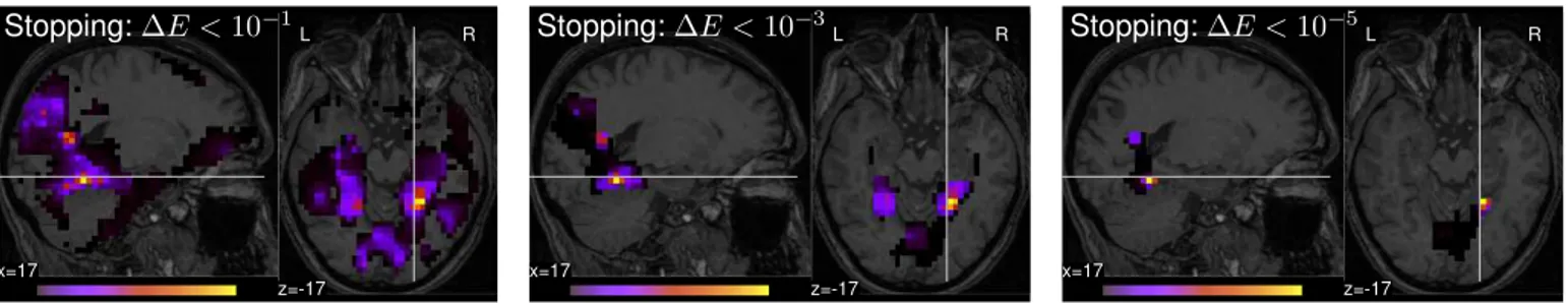
only for well-optimized solutions. As a result, the brain maps extracted vary significantly as a function of the tolerance on
the solver (see Fig.1).
In this contribution, we compare a comprehensive list of
solvers, all implemented with great care, for solving TV−ℓ1
regression with a focus on convergence time. First we state
the formal problem solved. In section III we present the
various algorithms. Experiments done and the results obtained
are presented in secions IV and V respectively. Section VI
concludes the paper with general recommendations.
II. FORMAL PROBLEM STATEMENT AND NOTATIONS
We denote by y∈ Rn the targets to be predicted, and X∈
Rn×p the brain images related to the presentation of different
stimuli.p is the number of voxels and n the number of samples
(images). Typically, p ∼ 103− 105 (for a whole volume),
while n ∼ 10 − 103. Let Ω ⊂ R3 be the 3D image domain,
discretized on a finite grid. The coefficients w define a spatial
map in Rp. Its gradient at a voxelω ∈ Ω reads:
∇w(ω) := [∇xw(ω), ∇yw(ω), ∇zw(ω)] ∈ R3, (1)
where∇u is the spatial difference operator along the u-axis.
Thus ∇ is a linear operator ∈ R3p×p with adjoint ∇T =
−div ∈ Rp×3p.∆ := ∇T∇ ∈ Rp×p is the Laplace operator.
TV−ℓ1regression leads to the following non-smooth convex
optimization problem [8]:
ˆ
w:= argmin
w
{E(w) := L(y, X, w) + αJ(w)}, (2)
where J(w) := θkwkℓ1+ (1 − θ)kwkT V is the
regulariza-tion and α ≥ 0 controls the amount of regularization. The
parameterθ ∈ [0, 1], also known as the ℓ1 ratio, is the
trade-off between the sparsity-inducing penalty ℓ1 (Lasso) and TV
(isotropic Total Variation):
kwkℓ1 := X ω∈Ω |w(ω)|; kwkT V := X ω∈Ω k∇w(ω)k2 . (3)
L(y, X, w) is the loss function. Here, we focus on the squared
loss and the logistic loss, defined e.g. in [6]. The squared loss
x=17 L R z=-17 Stopping:∆E < 10−1 x=17 L R z=-17 Stopping:∆E < 10−3 x=17 L R z=-17 Stopping:∆E < 10−5
Fig. 1. TV−ℓ1maps for the face-house discrimination task on the visual recognition dataset, with regularization parameters chosen by cross-validation, for
different stopping criteria. Note that the stopping criterion is defined as a threshold on the energy decrease per one iteration of the algorithm, and thus differs from the tolerance displayed in figure3. This figure shows the importance of convergence for problem (2), and motivates the need for a fast solver.
is natural for regression settings, where y is a continuous
variable, but it may also be used for classification [12].
The logistic loss is harder to optimize, but more natural for classification settings.
III. ALGORITHMS
In this section, we present the algorithms we benchmarked
for solving problem (2).
a) ISTA/FISTA: ISTA [10], and its accelerated variant
FISTA [11], are proximal gradient approaches: the go-to
meth-ods for non-smooth optimization. In their seminal introduction
of TV for fMRI, Michel et al. [6] relied on ISTA. The
chal-lenge of these methods for TV is that the proximal operator of TV cannot be computed exactly; we approximate it in an inner
FISTA loop [13], [6]. Here, for all FISTA implementations we
use the faster monotonous FISTA variant [13]. We control the
optimality of the TV proximal via its dual gap [6] and use a
line-search strategy in the monotonous FISTA to decrease the tolerance as the algorithm progresses, ensuring convergence
of the TV-ℓ1 regression with good accuracy.
b) ISTA/FISTA with backtracking: A key ingredient in
FISTA’s convergence is the Lipschitz constant L(L), of the
derivative of smooth part of the objective function . The tighter the upper bound used for this constant, the faster the resulting
FISTA algorithm. In FISTA, the main use ofL(L) is the fact
that: for any stepsize0 < t ≤ 1/L(L) and for any point z,
L(pt(z)) ≤ L(z) + rTt∇L(z) + 1 2tkrtk 2 2, where pt(z) := proxαtJ(z − t∇L(z)) and rt:= pt(z) − z (4)
In least-squares regression, L(L) is precisely the largest
singular value of the design matrix X. For logistic
regres-sion however, the tightest known upper bound for L(L) is
kXkkXTk (for example see Appendix A of [14]), which
performs very poorly locally (i.e, stepsizes ∼ 1/L(L) are
sub-optimal locally). A way to circumvent this difficulty is
backtracking line search [11], where one tunes the stepsizet
to satisfy inequality (4) locally at point z.
c) ADMM: Alternating Direction Method of Multipliers:
ADMM is a Bregman Operator Splitting primal-dual method for solving convex-optimization problems by splitting the objective function in two convex terms which are functions of
linearly-related auxiliary variables [15]. ADMM is particularly
appealing for problems such as TV regression: using the
variable split z ← ∇w, the regularization is a simple ℓ1/ℓ2
norm on z for which the proximal is exact and computationally cheap. However, in our settings, limitations of ADMM are:
• the w-update involves the inversion of a large (p × p)
ill-conditioned linear operator (precisely a weighted sum
of XTX, the laplacian∆, and the identity operator).
• the ρ parameter for penalizing the split residual z − ∇w
is hard to set (this is still an open problem), and though under mild conditions ADMM converges for any value
of ρ, the convergence rate depends on ρ.
d) Primal-Dual algorithm of Chambolle and Pock [16]:
this scheme is another method based on operator splitting.
Used for fMRI TV regression by [8], it does not require
setting a hyperparameter. However it is a first-order single-step method and is thus more impacted by the conditioning of the problem. Note that here we explore this primal-dual method only in the squared loss setting, in which the algorithm can
be accelerated by precomputing the SVD of X [8] .
e) HANSO [17]: a modified LBFGS scheme based on
gradient sampling methods [18] and inexact line-search. For
non-smooth problems as in our case, the algorithm relies on random initialization, to avoid singularities with high proba-bility. Here, we used the original authors’ implementation.
f) Uniform approximation by smooth convex surrogates:
ℓ1 (resp. TV) is differentiable almost everywhere, with
gra-dient w(ω)/|w(ω|))ω∈Ω (resp. −div(∇w/k∇wk2)), except
at voxels ω of the weights map where w(ω) = 0 (resp.
k∇w(ω)k2 = 0), corresponding to black spots (resp. edges).
A convenient approach (see for example [19], [20], [21], [22])
for dealing with such singularities is to uniformly approximate the offending function with smooth surrogates that preserve
its convexity. Given a smoothing parameterµ > 0, we define
smoothed versions of ℓ1 and TV:
kwkℓ1,µ:= X ω∈Ω p w(ω)2+ µ2 kwkT V,µ:= X ω∈Ω q k∇w(ω)k2 2+ µ2 (5)
These surrogate upper-bounds are convex and everywhere-differentiable with gradients that are Lipschitz-continuous with
constants1/µ and k∇k2(1/µ) = 12/µ respectively. They lead
to smoothed versions of problem (2):
ˆ
wµ:= argmin
w
{Eµ(w) := L(y, X, w) + αJµ(w)}, (6)
To solve (2), we consider problems of the form (6) with
µ → 0+: we start with a coarseµ (= 10−2, e.g) and cheaply
solve theµ-smoothed problem (6) to a precision ∼ µ using a
fast iterative oracle like the LBFGS [23]; we obtain a better
estimate for the solution; then we decreaseµ by a fixed factor,
and restart the solver on problem (6) with this solution; and
so on, in a continuation process [19] detailed in Alg.1.
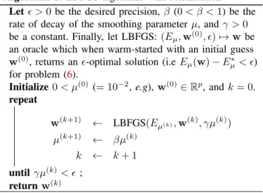
Algorithm 1: LBFGS algorithm with continuation
Letǫ > 0 be the desired precision, β (0 < β < 1) be the
rate of decay of the smoothing parameterµ, and γ > 0
be a constant. Finally, let LBFGS:(Eµ, w(0), ǫ) 7→ w be
an oracle which when warm-started with an initial guess
w(0), returns anǫ-optimal solution (i.e Eµ(w) − Eµ∗< ǫ)
for problem (6).
Initialize 0 < µ(0) (= 10−2, e.g), w(0)∈ Rp, andk = 0.
repeat w(k+1) ← LBFGS(Eµ(k), w(k), γµ(k)) µ(k+1) ← βµ(k) k ← k + 1 untilγµ(k)< ǫ ; return w(k)
This algorithm is not faster than O(1/ǫ): indeed a good
optimization algorithm for the sub-problem (6) isO(pLµ/ǫ)
[24], andLµ∼ 1/µ ∼ 1/ǫ. We believe that this bound is tight
but a detailed analysis is beyond the scope of this paper.
IV. EXPERIMENTS ON FMRIDATASETS
We now detail experiments done on publicly available data. All experiments were run full-brain without spatial smoothing.
g) Visual recognition: Our first benchmark dataset is a popular block-design fMRI dataset from a study on face and
object representation in human ventral temporal cortex [1]. It
consists of 6 subjects with 12 runs per subject. In each run, the subjects passively viewed images of eight object categories, grouped in 24-second blocks separated by intermittent rest periods. This experiment is a classification task: predicting the object category. We use a two-class prediction target: y encodes faces versus houses. The design matrix X is made
of time-series from the full-brain mask ofp = 23 707 voxels
overn = 216 TRs, of a single subject (subj1).
h) Mixed Gambles: Our second benchmark dataset is a study in which subjects were presented with mixed (gain/loss) gambles, and decided whether they would accept each gamble
[25]. No outcomes of these gambles were presented during
scanning, but after the scan three gambles were selected at random and played for real money. The prediction task here is to predict the magnitude of the gain and thus a regression on
a continuous variable [26]. The data is pooled across subjects,
resulting in 768 samples, each an image of 33 177 voxels. We study the convergence of the algorithms for parameters close to the optimal parameters set by 10-fold cross-validation to maximize prediction accuracy.
V. RESULTS:CONVERGENCE TIMES
Here, we present benchmark results for our experiments.
Figure 2 gives results for the logistic regression run on the
visual recognition dataset: convergence plots of energy as a function of time show that all methods are asymptotically
decreasing. Figure 2 left, shows the time required to give
a convergence threshold, defined as a given excess energy compared to the lowest energy achieved by all methods, for different choices of regularization parameters. Similarly, figure
3 shows convergence times for squared loss on both datasets.
For these figures, each solver was run for a maximum of 1 hour per problem. Solvers that do not appear on a plot did not converge for the corresponding tolerance and time budget.
For logistic loss, the most serious contender is algorithm1,
LBFGS applied on a smooth surrogate, followed by ADMM, however ADMM performance varies markedly depending on
the choice ofρ. For the squared loss FISTA and algorithm1are
the best performers, with FISTA achieving a clear lead for the larger mixed-gambles dataset. Note that in the case of strong regularization the problem is better conditioned, and first-order methods such as the primal-dual approach can perform well.
VI. CONCLUSIONS:APPROACHES TO PREFER
TV−ℓ1 penalized regression for brain imaging leads to
very high-dimensional, non-smooth and very ill-conditioned optimization problems. We have presented a comprehensive comparison of state-of-the-art solvers in these setting. Solvers were implemented with all known algorithmic improvements and implementation were carefully profiled and optimized.
Our results outline best strategies: monotonous FISTA with a adaptive control of the tolerance of the TV proximal op-erator, in the case of squared loss; smoothed quasi-newton based on surrogate upper-bounds of the non-smooth norms for logistic loss. While these algorithms are variants of existing approaches, we present here novel additions useful for the
TV or TV−ℓ1 settings. The fact that the smooth approaches
emerge as fast solvers on these non-smooth problems is not unexpected as i) the amount of regularization is small ii) the prevailing term is smooth and very ill conditioned, thus calling for second-order methods such as Newton or quasi-Newton.
For neuroimaging applications, our study has highlighted the need to converge to a good tolerance and the correspond-ing difficulties. Lack of good solver and explicit control of tolerance can lead to brain maps and conclusions that reflect
properties of the solver more than of the TV−ℓ1 solution.
Acknowledgments: This work was supported by the Human
Brain Project.
REFERENCES
[1] J. V. Haxby, M. I. Gobbini, M. L. Furey, A. Ishai, J. L. Schouten, and P. Pietrini, “Distributed and Overlapping Representations of Faces and Objects in Ventral Temporal Cortex,” Science, vol. 293, p. 2425, 2001. [2] Y. Kamitani and F. Tong, “Decoding the visual and subjective contents
of the human brain,” Nat. Neurosci., vol. 8, p. 679, 2005.
[3] J.-D. Haynes and G. Rees, “Decoding mental states from brain activity in humans,” Nat. Rev. Neurosci., vol. 7, p. 523, 2006.
[4] Y. Fan, N. Batmanghelich, C. M. Clark, and C. Davatzikos, “Spatial patterns of brain atrophy in MCI patients, identified via high-dimensional pattern classification, predict subsequent cognitive decline,” Neuroimage, vol. 39, p. 1731, 2008.
10−1 100 101 102 103 time (s) 10−5 10−4 10−3 10−2 10−1 100 101 102 103 104 105 e xce ss e n e rg y ADMM (ρ=1) ADMM (ρ=1e5) ADMM (ρ=1e11) ADMM (ρ=kXkkJk22) FISTA FISTA-BT HANSO ISTA ISTA-BT LBFGS 1e-3 0.10 1e-3 0.25 1e-3 0.50 1e-3 0.75 1e-3 0.90 1e-2 0.10 1e-2 0.25 1e-2 0.50 1e-2 0.75 1e-2 0.90 1e-1 0.10 1e-1 0.25 1e-1 0.50 1e-1 0.75 1e-1 0.90 102 103 C o n ve rg e n ce ti m e in se co n d s α ℓ1ratio
Fig. 2. TV−ℓ1 penalized Logistic Regression on the visual recognition face-house discrimination task. Left: excess energyE(wt) − E(wt)t→∞ as a
function of time. Right: convergence time of the various solvers for different choice of regularization parameters. Broken lines correspond to a tolerance of 100
, whilst full-lines correspond to10−2
. The thick vertical line indicates the best model selected by cross-validation.
1e-2 0.10 1e-2 0.25 1e-2 0.50 1e-2 0.75 1e-2 0.90 1e-1 0.10 1e-1 0.25 1e-1 0.50 1e-1 0.75 1e-1 0.90 1e0 0.10 1e0 0.25 1e0 0.50 1e0 0.75 1e0 0.90 α ℓ1ratio 101 102 103 C o n ve rg e n ce ti m e in se co n d s ADMM (ρ=1) ADMM (ρ=1e5) ADMM (ρ=1e8) ADMM (ρ=1e11) ADMM (ρ=kXkkJk22) Primal-Dual FISTA HANSO ISTA LBFGS 1e-3 0.10 1e-3 0.25 1e-3 0.50 1e-3 0.75 1e-3 0.90 1e-2 0.10 1e-2 0.25 1e-2 0.50 1e-2 0.75 1e-2 0.90 1e-1 0.10 1e-1 0.25 1e-1 0.50 1e-1 0.75 1e-1 0.90 102 103 C o n ve rg e n ce ti m e in se co n d s α ℓ1ratio
Fig. 3. TV−ℓ1penalized Least-Squares Regression. Left: on the visual recognition face-house discrimination task; Right: on the Mixed gambles dataset.
Broken lines correspond to a tolerance of100, whilst full-lines correspond to
10−2. The thick vertical line indicates the best model selected by cross-validation.
[5] M. K. Carroll, G. A. Cecchi, I. Rish, R. Garg, and A. R. Rao, “Prediction and interpretation of distributed neural activity with sparse models,”
NeuroImage, vol. 44, p. 112, 2009.
[6] V. Michel, A. Gramfort, G. Varoquaux, E. Eger, and B. Thirion, “Total variation regularization for fMRI-based prediction of behaviour,” IEEE
Transactions on Medical Imaging, vol. 30, p. 1328, 2011.
[7] L. Baldassarre, J. Mourao-Miranda, and M. Pontil, “Structured sparsity models for brain decoding from fMRI data,” in PRNI, 2012, p. 5. [8] A. Gramfort, B. Thirion, and G. Varoquaux, “Identifying predictive
regions from fMRI with TV-L1 prior,” in PRNI, 2013.
[9] A. Abraham, E. Dohmatob, B. Thirion, D. Samaras, and G. Varoquaux, “Extracting brain regions from rest fMRI with total-variation constrained dictionary learning,” MICCAI, 2013.
[10] I. Daubechies, M. Defrise, and C. De Mol, “An iterative thresholding al-gorithm for linear inverse problems with a sparsity constraint,” Commun.
Pure Appl. Math., vol. 57, no. 11, pp. 1413 – 1457, 2004.
[11] A. Beck and M. Teboulle, “A fast iterative shrinkage-thresholding algo-rithm for linear inverse problems,” SIAM Journal on Imaging Sciences, vol. 2, p. 183, 2009.
[12] J. A. Suykens, T. Van Gestel, J. De Brabanter, B. De Moor, and J. Vandewalle, Least squares support vector machines. World Scientific, 2002.
[13] A. Beck and M. Teboulle, “Fast gradient-based algorithms for con-strained total variation image denoising and deblurring problems,” Trans.
Img. Proc., vol. 18, p. 2419, 2009.
[14] C.-J. L. Guo-Xun Yuan, Chia-Hua Ho, “An improved glmnet for l1-regularized logistic regression,” Department of Computer Science
National Taiwan University, 2012.
[15] S. Boyd, N. Parikh, E. Chu, B. Peleato, and J. Eckstein, “Distributed
optimization and statistical learning via the alternating direction method of multipliers,” Fundations and Trends in Machine Learning, 2010. [16] A. Chambolle and T. Pock, “A first-order primal-dual algorithm for
convex problems with applications to imaging,” J. Math. Imaging Vis., vol. 40, p. 120, 2011.
[17] A. Lewis and M. Overton, “Nonsmooth optimization via BFGS,” 2008. [18] J. Burke, A. Lewis, and M. Overton, “A robust gradient sampling algo-rithm for nonsmooth, nonconvex optimization,” SIAM J. Optimization, vol. 15, pp. 751–779, 2005.
[19] J. Bobin, S. Becker, and E. Candes, “A fast and accurate first-order method for sparse recovery,” SIAM J Imaging Sciences, 2011. [20] Y. Nesterov, “Smooth minimization of non-smooth functions,” Math.
Program., vol. Ser. A 103, p. 127152, 2005.
[21] ——, “Excessive gap technique in nonsmooth convex minimization,”
SIAM Journal on Optimization, vol. 16, p. 235, 2005.
[22] A. Beck and M. Teboulle, “Smoothing and first order methods: A unified framework,” SIAM J. OPTIM., vol. 22, no. 2, pp. 557–580, 2012. [23] C. Zhu, R. H. Byrd, P. Lu, and J. Nocedal, “L-BFGS-B– Fortran
subroutines for large-scale bound constrained optimization,”
NORTH-WESTERN UNIVERSITY Department of Electrical Engineering and Computer Science, 1994.
[24] Y. Nesterov, “A method of solving a convex programming problem with convergence rate O(1/k2
),” Soviet Mathematics Doklady, 1983. [25] S. M. Tom, C. R. Fox, C. Trepe, and R. A. Poldrack, “The neural basis
of loss aversion in decision-making under risk,” Science, vol. 315, no. 5811, pp. 515–518, 2007.
[26] K. Jimura and R. A. Poldrack, “Analyses of regional-average activation and multivoxel pattern information tell complementary stories,”