Volume7, Issue 4 2007 Article1
A Causal Analysis of the R&D Interactions
between the EU and the US
Erdal Atukeren
∗between the EU and the US
∗
Erdal AtukerenAbstract
This paper examines the relationships between the aggregate R&D activities of the EU and the US using multivariate Granger-causality tests. Our estimation results indicate that the EU reacts positively to increases in R&D productivity in the US. On the other hand, R&D activity in the EU is a direct Granger-cause of both R&D and labour productivity in the US, and the effects are negative. It was shown in the literature that the US reacts submissively to successful Japanese R&D. We extend the literature by demonstrating that the US also reacts submissively to increased R&D effort in the EU.
KEYWORDS: R&D races, productivity spillovers, Granger-causality, EU’s Lisbon targets
∗Earlier versions of this paper were presented at the International Conference on Policy Modelling (ECOMOD) in Istanbul (Turkey) in June 2005, at the “Workshop on Innovation, R&D, and Adop-tion of New Technology” at the Christian Albrects University in Kiel (Germany) in June 2006, and at the Canadian Economic Association annual meetings in Halifax (NS, Canada) in June 2007. I would like to thank the participants of these sessions, Spyros Arvanitis, Kenneth Carlaw, and two anonymous referees of this journal for their valuable comments and suggestions. Needless to say, the responsibility for any errors and omissions is mine.
I. INTRODUCTION
In their Lisbon summit in 2000, the Ministers of the European Council declared the goal of turning the European Union (EU) into “…the most competitive and dynamic knowledge-based economy in the world by 2010”. Among various targets to achieve this aim, the ratio of spending on research and development (R&D) activity was envisaged to increase from about 1.9 per cent in 2000 to three per cent in 2010. This target was emphasised again in the Barcelona meeting of the European Council in March 2002. As of 2007, the progress made towards meeting the Lisbon target on R&D has been slow and partly impeded by the politics of the allocation of expenditures in the EU budget.
Historically speaking, the ratio of overall spending on R&D (public and private sources) to GDP in the EU has varied between 1.6 and 2 per cent since the beginning of 1980s. On the other hand, this ratio was as high as three per cent in Japan and generally above 2.5 per cent in the United States of America (US). Furthermore, the R&D spending to GDP ratio showed a secular increase both in the US and in Japan since 1996 while the R&D spending/GDP ratio stagnated in the EU. In this context, the ambitious R&D target set by the European countries is a signal of showing aggressive reaction – at least at the policy making level – first of all not to lag behind and then to overtake the R&D (location) leadership. If successful, this policy should help enhance the EU’s long-term economic growth potential.1 Putting the political and economic realism of the EU’s R&D targets aside, the EU’s stated willingness to make an aggressive move to match the already higher and increasing level of R&D activities in other countries has game-theoretic implications.2
1
The link between R&D activity and economic performance has long been recognised. Schumpeter, for example, put forth the process of “creative destruction” as an engine economic growth. More recently, R&D is formally given a central role in various variants of the endogenous growth theory as a driver of technological progress and long-term economic growth. The introduction of R&D as a driver of economic growth is an important development since it connects the economic growth process further with micro foundations, bearing implications for economic and public policy. See Lucas (1988), Romer (1990), Grossman and Helpman (1991), Grilliches (1992), Jones (1995), Aghion and Howitt (1998), and Segerstrom (1998). See also Lingens (2005) for a short discussion of the various versions (the first and second generations) of endogenous growth models and their policy implications. Goel and Rich (2005) provide a neat representation of the various aspects of the markets for R&D activity.
2
This is indeed a race for becoming an attractive R&D location since R&D activities in an economy (say, the EU, the US, or Japan) are undertaken not only by the nationals but also by the affiliates of foreign companies or as multinational research joint ventures. Kuemmerle (1999) studies the factors that determine the multinationals’ decision to invest in R&D abroad. The home-base-exploiting (HBE) foreign direct investments (FDI) are found to be related to the relative attractiveness of the target market. The home-base-augmenting (HBA) FDI, on the other hand, correlates with the “…relative commitment to R&D of private and public entities in the target
While R&D races and games among firms (e.g., whether or not to innovate, when to innovate, formation of research joint ventures, etc.) and government policies towards the protection of inventions through patent policy are well-discussed in the industrial organisation literature, the direct relationship between the R&D activities of two countries or trading blocks has received less attention. An early exception is Scherer (1991) who examined the case of an “R&D race” between the US and Japan by means of bivariate Granger-causality tests. Scherer’s findings illustrated that the US firms reacted submissively, rather than aggressively, to the market penetration through R&D success by Japanese firms.3
In this context, a submissive reaction by a firm (say, “A”) to the R&D efforts by others (say, “B”) is said to occur when “A” decides to reduce its R&D budget/efforts and shifts resources rather into non-R&D physical capital investments or into marketing and advertising in response to increased R&D effort by “B”. It is well documented in the business and industrial organisation literature that both R&D and marketing & advertising expenditures influence sales positively (e.g., Brenner and Rushton, 1989) and that there is a trade-off between R&D and marketing spending given the budget constraints (Ko, 2005). Thus, the submissive reaction discussed above might indeed be compatible with profit maximisation since what is at stake from a firm’s perspective is the sales figures. When a firm cannot (or decides not to) match the innovations made by the competitors, it may well increase its marketing & advertising spending in an attempt to increase its sales. The optimisation problem is, of course, a dynamic one. In the long-term, the myopic behaviour of shifting resources into marketing at the expense of R&D activity may lead to an inferior market position.
Scherer’s (1991) finding that the US displayed a submissive reaction to increases in Japanese R&D has been supported by a number of subsequent studies (Park, 1995; Eaton and Kortum, 1996; and Blonigen and Slaughter, 2001; among country, as well as with the level of human resource pool and the level of scientific achievement in relevant sciences.” (Kuemmerle, 1999: 18)
3
This example illustrates the conceptual suitability of Granger’s (1969) causality test and its variants as an empirical tool to investigate the nature of R&D races and spillovers, e.g. the aggressive vs. submissive reaction of one country to an increase in another country’s R&D efforts as well as the causal nature of the dynamic interaction between R&D and domestic economic activity. In the literature on R&D, there exist a number of studies that use Granger-causality tests to examine the interactions between physical capital accumulation and R&D activity, the relationship between total productivity growth and R&D at the aggregate or industry level, the effects of government policies and subsidies on private sector R&D, and the interactions between publicly and privately funded R&D. The following papers, among others, cover some of these topics: Verspagen (1995), Colombo and Garrone (1996), Frantzen (1998), Chiao (2001), Neelankavil and Alaganar (2003), Guellec and van Pottelsberghe de la Potterie (2003), Garcia-Quevedo (2004), Kim and Lee (2004), and Greunz (2004).
others).4 More recently, Luintel and Khan (2004) used cointegration analysis and showed that international R&D spillovers could indeed be costly for the US. At the macro level, the cost of not responding to competitors’ R&D moves aggressively enough could be felt first as a loss of export share in the world markets for high technology goods (i.e., exports originating from R&D intensive industries). In the longer run, lagging behind in innovation activities should also reflect itself in relatively lower economic performance and productivity growth rates.
Assessing the direction and the sign of the causality in R&D interactions between firms/countries is a complicated task since innovation activity leads to knowledge spillovers. These spillovers mainly stem from the imperfect appropriability of rents from innovations and diffuse through international trade, foreign direct investments, imitation, and labour mobility, among other channels.5 As such, they occur not only within the home country but also across countries. Indeed, firms (domestic and/or foreign) may need to undertake catch up investments in R&D capability just to be able to make good use of the newly acquired technology from other firms since even sheer imitation requires the reverse engineering and reconstruction of the new product.6 This is in line with the argument that absorptive capacity plays a role in determining the extent of R&D spillovers (Carlsson and Mudambi, 2003).
R&D is intrinsically a risky business. Increased spending on R&D activities does not guarantee a successful outcome – at least immediately. Thus, there exists a phenomenon of “dry holes” in the nature of R&D activities. Hence, the actual results of R&D games are not easy to predict due to the inherent uncertainties and information asymmetries associated with innovation activities. In sum, the possibility of an aggressive or a submissive reaction, coupled with the particularities of the nature of innovation activity, makes the sign of the effects of R&D efforts by a firm/country on the R&D efforts of others indeterminate. Then, a deeper look into the nature of causality in the recent history of the R&D interactions between the EU and the US is especially important in view of the EU’s decision to set explicit R&D spending targets to counter the US’s R&D lead.
4
Bernstein and Mohnen (1998) estimate that there are positive R&D spillovers from the US to Japan but the conserve is not true.
5
See Coe and Helpman (1995), Coe, Helpman and Hoffmaister (1997), and Engelbrecht (1997a, 1997b). See also Hejazi and Safarian (1999) and Lewer and van den Berg (2003) for a discussion of the impact of foreign trade and foreign direct investment on R&D spillovers and economic growth.
6
This paper investigates the direction and the sign of causality in the international and domestic effects of R&D activity in the European Union (EU15 – i.e., the EU before the enlargements in 2004 and 2007) and the United States of America in a multivariate framework. The analysis uses annual data on R&D productivity and labour productivity for the 1979-2002 period. In particular, we test: 1) whether changes in the R&D effort in the EU Granger-cause a response in the R&D activity by the US, and if so, whether the reaction is aggressive or submissive; 2) whether changes in the R&D effort in the US Granger-cause an R&D response in the EU, and if so, whether this reaction is aggressive or submissive.
The rest of the paper is organised as follows. We first discuss the data and the methodology. Then, we present the empirical results and puts them in perspective with respect to the observed productivity differentials between the US and the EU. Conclusions follow.
II. DATA AND METHODOLOGY II.A DATA ISSUES
The most commonly employed measure of productivity in the studies of R&D spillovers is total factor productivity (TFP). The TFP is calculated as a residual from an aggregate production function, such as Y = AKαL(1-α) , where Y is output, K is capital stock, L is labour input, A is a technology parameter, and 0<α<1 is an elasticity parameter. In principle, one can obtain the estimates for TFP given the capital and labour input and the value of α. However, there are numerous assumptions behind this approach and the estimates of technological progress hence obtained are model dependent. In addition, any adjustments made by the national statistical agencies to account for quality changes in the capital stock may reduce or eliminate the impact of embodied technical progress. Furthermore, the estimation of capital stock is problematic in itself. Also, since we take the EU as an overall entity or a trading block of 15 countries, it might be erroneous to combine the capital stock figures calculated by different national statistical offices.
Labour productivity is an alternative measure to TFP. It is not dependent on the assumptions of a theoretical model and it does not require capital stock estimates.7 Furthermore, various versions of labour productivity are used in making cross-country comparisons of economic growth and development. In a study of knowledge spillovers through trade, Falvey, Foster, and Greenaway
7
See Sargent and Rodriguez (2000) and Lipsey and Carlaw (2004) for a further discussion the issues in the measurement of technological progress.
(2002, 2004) argue in favour of a productivity measure (GDP per capita), which is rather related to labour productivity than the TFP. In view of the above considerations, we also take labour productivity as a measure of domestic productivity developments in the EU and in the US.
The choice of the R&D variable is made as follows. In the literature, the R&D activity is generally quantified in terms of expenditures. The EU indeed set its target in terms of R&D expenditure/GDP ratio. Nevertheless, there are a number of problems in using R&D expenditure data. First of all, the timing and the intensity of successful outcomes from increased R&D expenditures involve uncertainties. Secondly, the definition of what is “high tech” or “R&D-intensive good” changes overtime. Furthermore, the R&D expenditure figures from the OECD’s Main Science Indicators database contain many breaks, making them unsuitable for long-term time series analysis purposes. It may be possible to pool the R&D expenditure data for shorter periods of time, where they are consistent, and use panel data methods. Indeed, a large share of the studies in the literature that uses R&D expenditure data employs pooled time-series – cross-section data and conducts panel cointegration tests. The panel data techniques are useful especially when the span of data is too small to conduct meaningful cointegration and causality tests between the variables of interest. However, they are subject to more stringent assumptions about the data generating processes due to pooling. In a study of R&D spillovers across G10 countries, Luintel and Khan (2004: 909) conclude that it is not appropriate to pool their data since “…long-run spillover elasticities differ significantly among sample countries; and panel estimates, in general, do not correspond to country-specific parameters. Thus, panel tests appear to conceal important cross-country differences in knowledge spillovers.”
Since this paper is particularly aiming at causally investigating the foreign and domestic effects of R&D activities in the EU and in the US, we need consistently compiled time series data with a reasonably long span to run the multivariate Granger-causality tests. Therefore, we make use of the University of Groningen’s “Growth and Development Centre, 60-Industry Database (GGDC_60), version February 2005”. The GGDC_60 reports national-accounts-based value-added data, standardised by the ISIC (revision 3) classification system, for a large number of OECD countries for the 1979-2002 period. Under the ISIC rev. 3, “Section 73” is the “research and development” activity from all sources.8 We select this entry to as a measure of the economy-wide R&D activity.
Both the value-added in R&D activities and in the total economy are measured in real terms (at 1995 constant prices). They are further adjusted for differences in employment levels and indexed as 1995=100 to make the data comparable across countries and in levels. The resulting four variables are the real
8
value-added per worker (labour productivity) in the R&D activities and in the total economies of the EU (EURD, EULP) and the US (USRD, USLP). Since labour productivity growth is also due to other factors than R&D, we also take the deviations of these series from their 1979-2002 trend growth. Figures 1-4 show the graphs of the series in question.
FIGURE 1. LABOUR PRODUCTIVITY IN THE US (USLP)
-4 -2 0 2 4 6 80 90 100 110 120 80 82 84 86 88 90 92 94 96 98 00 02 USLP in Levels (1995=100) Trend (1979-2002)
USLP (Deviation from Trend)
FIGURE 2. R&D PRODUCTIVITY IN THE US (USRD
)
-10 -5 0 5 10 80 90 100 110 120 130 80 82 84 86 88 90 92 94 96 98 00 02 USRD in Levels (1995 = 100) Trend (1979-2002)
USRD (Deviation from Trend)
As Figures 1 and 2 show, there is a coincidence between the general productivity slump (1989 – 1998) in the US and the slump in the real value-added per worker in R&D activities (1985 – 1996). Furthermore, there appears to be a leading effect from R&D activities. In the case of EU, the situation is not clear
(Figures 3 and 4). However, a time-series analysis of the lead-lag relationships may still tell a different story than the visual first impressions.
FIGURE 3. LABOUR PRODUCTIVITY IN THE EU15 (EULP)
-4 -2 0 2 4 6 60 70 80 90 100 110 120 80 82 84 86 88 90 92 94 96 98 00 02 EULP in Levels (1995=100) Trend (1979-2002)
EULP (Deviation from Trend)
FIGURE 4. R&D PRODUCTIVITY IN THE EU15 (EURD)
-15 -10 -5 0 5 10 60 70 80 90 100 110 120 80 82 84 86 88 90 92 94 96 98 00 02 EURD in Levels (1995 = 100) Trend (1979-2002)
EURD (Deviation from Trend)
When it comes to the relationship between the deviation of the value-added in R&D activities per worker from its long-run trend in the US and the EU,
there indeed appears to be a negative relationship.9 This is illustrated as a scatterplot with a linear regression line in Figure 5.
FIGURE 5. SCATTERPLOT OF THE EU’S AND THE US’S R&D PRODUCTIVITIES -12 -8 -4 0 4 8 12 -12 -8 -4 0 4 8 12 EURD U S R D USRD vs. EURD
It should be noted that Figure 5 displays the bivariate relationship between the productivity in the EU’s and the US’s R&D activities without controlling for any third variables. The direction of causality cannot be deduced by using (partial-) correlation analysis. Then, the question is whether the observed negative relationship between the USRD and EURD is spurious or whether it shows the existence of a submissive reaction by one of the players – e.g., the US’s R&D hurting the EU’s or vice versa.
9
A negative correlation between the R&D activities of the EU and the US is also reflected by other indicators. For instance, the EU’s average share in the highly cited (top 1%) publications increased from 35.42% to 37.12% between the 1993-1997 and 1997-2001 periods, while the US’s share declined from 37.46% to 34.86% in the same periods. Similarly, the EU’s share of citations in the top 1% cited publications increased from 36.57% to 39.3% and the US’s share registered a decline from 39.3% to 32.85% between the 1993-1997 and 1997-2001 periods. See King (2004) for further details and comparisons.
II.B METHODOLOGY: TESTING FOR GRANGER-CAUSALITY IN A MULTIVARIATE FRAMEWORK
Granger’s (1969) definition of causality between two weakly stationary stochastic variables X and Y is as follows. X is said to Granger-cause Y if and only if Y can be better predicted by using X in addition to the history (lags) of Y and all other relevant information. In the bivariate case, this definition takes the following form in practice:
ε
γ
β
α
1j t-j 1t q 1 = j j -t 1j p 1 = j 1 t=
+
y
+
x
+
y
Σ
Σ
(1)ε
γ
β
α
j t-j t s 1 = j j -t j r 1 = j t=
+
y
+
x
+
x
2Σ
2Σ
2 2 (2)where: α’s are constant terms; β’s and γ’s are parameters to be estimated; p, q, r, and s are lag-lengths; and
ε
it are well-behaved error terms. In equation (1) ifΣγ
1j ≠ 0, then X Granger-causes Y. Granger-causality from Y to X can be similarly defined. The practical problem with the above equations is how to choose the optimal lag-lengths (p,q,r,s). This is an important consideration since the results from Granger-causality tests are generally sensitive to the specification of the test equation. Granger (1969) used fixed lags, i.e., p=q=r=s. In later versions of the Granger’s causality test, flexible lag-lengths were used, e.g., Hsiao (1979, 1982). In this study, we use the subset autoregression and transfer function approach which includes only the significant lags in the specification of equations (1) and (2) as suggested by Penm and Terrel (1984) and Kang (1989). Using the subset transfer function methodology has a further relevance in the context of empirical modelling of the effects of R&D activity. As discussed earlier, there might exist “dry holes” in the relationship between R&D and economic activity (Rouvinen, 2002). That is, not every increase in R&D effort necessarily immediately reflects itself into higher productivity in the economy. At times, there might be no visible effects, or the effects are small and unclear. But, they accumulate (e.g., learning effects even from unsuccessful attempts) and may show themselves after a long lag, or perhaps after “…some promising discovery.” (Rouvinen, 2002: 125). Then, the subset transfer function approach that suppresses the insignificant lags and allows for the possibility of including distant but significant lags into the specification is conceptually well-suited for empirically addressing the phenomenon of “dry holes”.For the selection of the optimal lag specifications in subset autoregressions and subset transfer functions, we use Schwarz’s (1978) “Bayesian Information Criterion (SBIC)”. SBIC is given by the formula: SBIC = (ESS/T)*T(k/T), where ESS is the error sum of squares from estimation of the model in question, T is the
sample size, and k is the number of estimated parameters in the model. Conceptually, SBIC is derived from Bayesian foundations. As such, it is an attempt to find the most probable model for the data at hand.
The detection of Granger (non-) causality from X to Y even in a bi-variate framework has important implications. According to Hsiao (1982), for X to be a direct cause of Y, X should cause Y in all settings: bi- and multi-variate. Furthermore, if X causes Y only indirectly via another variable Z, X should still cause Y when Z is not in the equation. Nevertheless, if Z is a common cause of both X and Y, and if there is no other direct or indirect relationship between X and Y, one may detect Granger-causality between X and Y in the absence of Z. The detected causality in this case would be spurious. In our study, we start with the examination of Granger-causality in the bivariate case, but extend the analysis into a 4-variable framework subsequently. Still, we qualify our findings as prima
facie since the missing cause problem is not necessarily solved in a multivariate framework.
Analysing the causal relationships among the variables of interest in a multivariate framework is a complex task due to any indirect linkages and possible spurious relationships. For example, consider the case where a variable X Granger-causes Y in a trivariate system (i.e., in the presence of a distinct variable Z) but not in a bivariate relationship. Hsiao (1982) calls this as “Type I spurious causality”. This may be a misnomer since the Z variable indeed acts as a catalyst or as a co-requisite condition for the causal relationship between X and Y to hold. In order to conclude in favour of non-causality from X to Y in a multivariate setting, X should not cause Y in a bivariate setting and, in addition, X should not be a (direct) cause of any variable that in turn causes Y. Further definitions can be found in Hsiao (1982). See also the Appendix to this study for a parameterised extension of Hsiao’s (1982) definitions in a 4-variable framework.
Another complication that arises in testing for Granger-causality is the following possibility: even if the introduction of X (say, with lags 1 and 2) over the best univariate specification for Y leads to a lower forecast error variance of Y (i.e., X Granger-causes Y), the estimated coefficients on lag 1 and 2 may carry opposite signs and cancel out, or their sum may not be statistically significant. In this case, it would be wrong to conclude that X does not cause Y since the conditions for Granger-causality are still fulfilled. This case, discussed in Sturm and De Haan (1998) among others, is called “neutrality”.
In addition, the following case may also be encountered in a 4-variable system consisting of Y, X, W, and Z. That is, one runs the Granger-causality test between X and Y first in a bivariate relationship, secondly in a system when W is present (X,Y,W), thirdly in a system when Z is present (X,Y,Z), and finally when all four variables are in the system (X,Y,W,Z). Now, let us assume that X is found to be a direct cause of Y (that is, X casuses Y in all settings), but the sign of the
estimated coefficients changes from specification to specification. Then, one must conclude that the relationship between X and Y is not robust in different specifications despite the findings of direct causality in the Granger-Hsiao sense. III. EMPIRICAL FINDINGS
Following the above discussion of the data and the methodological details and problems, we now turn to the examination of the Granger-causal links between the four variables described and graphically displayed earlier: EURD, EULP, USRD, and USLP. We are especially interested in finding out whether there are cases of “direct causality” between these variables. In running the Granger-causality tests, we first test for the time series properties of the variables in question using the augmented Dickey-Fuller (ADF), Phillips-Perron (PP), and the KPSS unit root tests. Note that the null hypothesis is non-stationarity in the ADF and PP tests, while the KPSS takes the null hypothesis as stationarity. The test results shown in Table 1 indicate that all series are stationary.
TABLE 1. UNIT ROOT TEST RESULTS
EURD EULP USRD USLP
ADF (levels) -2.781663*** [N,4] -3.514640*** [N,1] -3.300224*** [N,0] -1.956874** [N,4] ADF (1st Differences) -3.681901*** [N,0] -2.435185** [N,0] -7.207506*** [N,0] -3.786142*** [N,0] PP (Levels) -2.040573** [N,3] -2.413733** [N,2] -3.247849*** [N,1] -1.176495 [N,2] PP (1st Differences) -3.721546*** [N,2] -2.410303** [N,2] -8.501124** [N,6] -3.789211*** [N,1] KPSS (Levels) 0.160017 [C,3] 0.116081 [C,3] 0.170184 [C,2] 0.145178 [C,3] KPSS (1st Differences) 0.324349* [C,2] 0.290246 [C,2] 0.270488 [C,7] 0.432268 [C,2]
ADF: Augmented Dickey Fuller test, PP: Phillips – Perron Test, KPSS: Kwiatkowski-Phillips-Schmidt-Shin test. N: no trend and no intercept in the specification, C: intercept but no trend in the specification. The numbers in the square brackets indicate the lag-length in the ADF test, and the bandwidth in the PP and KPSS tests. (***), (**), and (*) indicate, respectively that the null hypothesis can be rejected at 1%, 5% and 10% statistical significance levels.
Next, we examine the bivariate causal relationships using the system shown in equations (1) and (2). The generic variable names X and Y are replaced with a pair of the EURD, EULP, USRD, USLP variables in the actual test. The lag-lengths are selected through a subset autoregression and transfer function methodology as discussed earlier. The maximum lag-length was set to six. This is in line with Ravenscraft and Scherer (1982) who calculate that the mean lag for
the R&D efforts to show their effects (on industrial profitability) is 4 to 6 years. Our choice has also been necessitated by the available number of observations (1979-2002, i.e., 23 years) and the number of variables (four) in our study. For example, if we were to estimate a vector autoregression (VAR) that is formed without a subset autoregression and transfer function methodology, we would be able to use at most 4 lags – leaving only 2 degrees of freedom in each equation, not a healthy choice for making statistical inferences. Nevertheless, the subset methodology eliminates the insignificant or redundant parameters and leads to more efficiency in estimation in addition to allowing for the inclusion of more distant but possibly significant lags in the specification. Table 2 shows the details of the resulting specifications and the SBIC values in the bivariate model. The headers “Caused Variable” and the “Causing Variable” can be read as the Y and X variables, respectively, in line with equations (1) and (2)
TABLE 2. BIVARIATE GRANGER-CAUSALITY TEST RESULTS
Caused variable: Univariate Specification SBICUV Causing variable:
Transfer Sign & Function Sig. Level
SBIC2V EURD 1,4,5 4.673850 EULP 4 (+) 4.735744 EURD 1,4,5 4.673850 USRD 2 (+)** 4.512524 ‡ EURD 1,4,5 4.673850 USLP 1,6 (+)*** 4.585471 ‡ EULP 1,4 2.563014 EURD 1,3,4 (-) 2.501711 ‡ EULP 1,4 2.563014 USRD 1,6 (+)*** 2.401400 ‡ EULP 1,4 2.563014 USLP 2,5 (-) 2.511896 ‡ USRD 6 5.952995 EURD 1,3 (-)*** 5.664985 ‡ USRD 6 5.952995 EULP 3,4,6 (-)*** 5.871018 ‡ USRD 6 5.952995 USLP 1,5,6 (-)*** 5.633191 ‡ USLP 1,5 2.692500 EURD 1,2,3 (-)** 2.336714 ‡ USLP 1,5 2.692500 EULP 1,2,3 (-) 2.693477 USLP 1,5 2.692500 USRD 3 (+) 2.725659
Source: Author’s calculations. Detailed estimation results and regression diagnostics are available upon request. (***), (**), and (*) indicate respectively that the coefficient(s) is/are (jointly) significant at 1%, 5% and 10% statistical significance levels. (‡) indicates that the SBIC2V <
SBICUV for the entry in question.
A brief explanation about the entries in Table 2 is in order. For example, the entry for the case of EURD and USRD (the second row in the table) should be read as follows: EURDt = α + β1EURDt-1 + β2EURDt-4 + β3EURDt-5 + β4USRDt-2, with the resulting univariate (for EURD) Schwarz BIC (SBICUV) value of 4.673850 and a subset bivariate transfer function (TF) SBIC value (SBIC2V) of 4.512524. Since the SBIC2V < SBICUV, the USRD can be said to Granger-cause EURD in a bivariate specification. The other entries can be interpreted similarly.
Table 3 presents the qualitative summary of the results from the bivariate Granger-causality. In reading the entries in Table, it should be noted that “None” means no Granger-causality is detected and (.) indicates there is Granger-causality between the variables in question and shows the sign of the relationship in parentheses, where the sign is confirmed as a result of joint-significance tests (Wald) in case of multiple lags entering the specification. A more complicated case arises when there is indeed Granger-causality from the causing variable to the caused one, but the signs on the lags of the causing variable do not turn out to be jointly significant (as they positive and negative values may have cancelled out each other). This case is denoted by “Neutrality”.
TABLE 3. SUMMARY OF THE RESULTS FROM THE BIVARIATE GRANGER-CAUSALITY TESTS
←
Causing Variables
Caused Variables ↓ EURD EULP USRD USLP
EURD --- None (+) (+)
EULP Neutrality --- (+) Neutrality
USRD (-) (-) --- (-)
USLP (-) None None ---
Source: Author’s calculations based on the results reported in Table 2.
The qualitative findings from the bi-variate Granger-causality tests provide a first glimpse into the causal relationships among our set of variables. First of all, the impact of an increase in the productivity of R&D activity (above the long-run trend) in the EU is found to have negative effects on the R&D and overall labour productivity in the US. On the other hand, the EU appears to be positively affected from an increase in the US’s R&D productivity. Similar to the findings on the effects of Japanese R&D efforts on the US, the R&D efforts in the EU also appear to be costly for the US.
When it comes to the effects of R&D on the domestic sectors, no significant or persistent effect is found either in the EU or in the US. In addition, the impact of an increase in labour productivity (above the long-run trend) does not appear to spill into the R&D efforts in the case of EU. In the US, the impact is indeed negative. Since labour productivity may increase also due to improvements in human capital quality or substitution of physical capital for labour, the firms may be in a position to cut down their R&D budgets and shift resources into marketing and advertising and/or compete in the domestic or
international markets through productivity increases brought about by other means. Finally, there is no spillover effect from the EU’s labour productivity on the US. There is some indication of spillovers from the US labour productivity to the EU’s, but the overall effect is neutral.
Keeping these findings in mind, we now extend the causal analysis into 3- and 4-variable settings. The following are the trivariate systems to be investigated: 1) EULP, EURD, USRD, 2) EULP, EURD, USLP, 3) EULP, USRD, USLP, and 4) EURD, USRD, USLP. In the 4-variable system, we estimate four models, each one explaining one of the above variables (as the dependent variable) on its own lags and on the lags of the three remaining variables.
In multivariate models, the choice of the lag-lengths and thus determining the optimal model specification becomes rather complicated. We addressed this problem as follows. First, we used the bivariate specifications (say, EULP and EURD) as the basis to introduce the third variable (say, USRD). The optimal specification was found through minimising the SBIC criterion resulting from different lag-length specifications. This procedure was repeated once more by changing the order of the variables in the bivariate specification (i.e., EURD and EULP with USRD again being the third variable), and the resulting SBIC value was noted. Then, comparing the SBIC values from the two models, we picked the one with the lowest value as the basis for the 4-variable model. This is in line with the principle that the optimal specification should be robust to variable orderings. Next, we entered the fourth variable into the systems. A similar methodology to the trivariate case is again used to select the model with the lowest SBIC value. The equations of the 4-variable case and a description of the conditions to evaluate the causal relationships among the variables are given in the Appendix. The optimal specifications and the resulting SBIC values from the trivariate and 4-variate models are presented in Tables 4 and 5, respectively.
TABLE 4. TRIVARIATE GRANGER-CAUSALITY TEST RESULTS
A) EULP, EURD, USRD
EULP(t-i) Sign EURD(t-i) Sign USRD(t-i) Sign SBIC3V
EULP(t) 1,4 1,3,4 (-) 2,3,4,6 (-) 1.821814 EURD(t) 1,5,6 (-) 1,4,5 1,2,3,6 (+) 3.973010 USRD(t) 6 (-) 1,3 (-) 6 4.871124
B) EULP, EURD, USLP
EULP(t-i) Sign EURD(t-i) Sign USLP(t-i) Sign SBIC3V
EULP(t) 1,4 1,3,4 (N) 1,2,4,6 (N) 2.437927 EURD(t) 1,4 (N) 1,4,5 1 (+) 4.292234 USLP(t) 2 (+) 1,2,6 (+) 1,5 2.200939
C) EULP, USRD, USLP
EULP(t-i) Sign USRD(t-i) Sign USLP(t-i) Sign SBIC3V
EULP(t) 1 1,2,3,4,5,6 (-) 2,5 (+) 1.540702 USRD(t) 6 (-) 6 3,6 (-) 5.253640 USLP(t) 1,2,3 (N) 1 (+) 1,5 2.764862
D) EURD, USRD, USLP
EURD(t-i) Sign USRD(t-i) Sign USLP(t-i) Sign SBIC3V
EURD(t) 1,4 4,6 (+) 1,6 (+) 4.385553 USRD(t) 1,3 (-) 6 3,4 (+) 5.064726 USLP(t) 1,2,3 (-) 2 (-) 1 1.846757 Source: Author’s calculations. The sign of the estimated coefficients are shown under the header “Sign” in parentheses (.) only if they are (jointly) statistically significant at least at 5 per cent level. (N) stands for the cases of “neutrality”.
The entries in Table 4 can be read in a similar way to Table 2. For example, the trivariate system involving EURD, USRD, and USLP (first entry under D) is specified as EURDt = α + β1EURDt-1 + β2EURDt-4 + β3USRDt-4 + β4USRDt-6 + β5USLPt-1 + β6USLPt-6 with the resulting Schwarz BIC (SBIC3V) value of 4.385553. Note that the SBIC3V value is less than the bivariate specification between the EURD and the USRD (SBIC2V = 4.512524). The sum of the coefficients (β3 + β4) on USRD is positive, as indicated in parentheses. They are found to be jointly significant by means of the Wald test. The same case is also established for the sign and the joint significance of the (β5 + β6) coefficients on the USLP variable. These findings indicate that EURD is Granger-caused by USRD and USLP and the signs of these causal relationships are positive. The (N) sign in the Table indicates that the sum of the estimated coefficients is not statistically different than zero, but the SBIC value obtained from the trivariate specification is less than the bi variate specification.
The entries in Table 5 can also be read similar to those in Table 4, but the specifications are extended into a 4-variate framework. SBIC4V denotes the value of the Schwarz BIC in the best 4-variate transfer function specification.
TABLE 5 THE SPECIFICATION AND THE ESTIMATION RESULTS OF THE 4-VARIATE MODEL
EURD(t-i) Sign USRD(t-i) Sign EULP(t-i) Sign USLP(t-i) Sign SBIC4V
EURD 1,4,5 2 (+) 1,5,6 (-) 1,4 (+) 3.693182 USRD 3,4,6 (-) 6 1,5,6 (+) 1,5,6 (-) 3.994254 EULP 4,6 (N) 1,2,3,4,5,6 (-) 1,4 2,5 (+) 0.694562 USLP 1,2,6 (-) 3 (+) 5,6 (-) 1,5 1.588105 Source: Author’s calculations. The sign of the estimated coefficients are shown under the header “Sign” in parentheses (.) only if they are (jointly) statistically significant at least at 5 per cent level. (N) stands for the cases of “neutrality”.
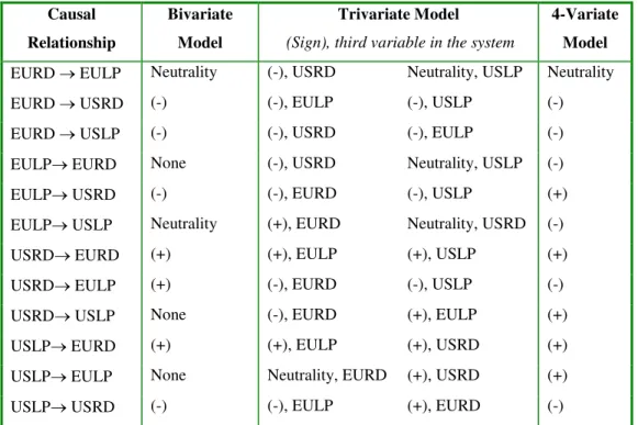
Table 6 presents the summary of all Granger-causality test results from bi-, tri-, and 4-variate models in qualitative terms. The results presented in Table 6 provide a rich ground for discussion both in terms of possible linkages (or lack thereof) and also the status of the causal relationships. For example, the only robust results for both the existence of a causal relationship and its estimated sign are obtained for: (1) EURD → USRD (-), (2) EURD → USLP (-), (3) USRD → EURD (+), and (4) USLP→ EURD (+), where the “→” sign shows the direction of Granger-Hsiao causality and the (.) shows the sign of the causal relationship. In the remaining cases, the presence of causal linkages and / or their direction are not found to be invariant to the exclusion and inclusions additional variables. These relationships appear to be spurious and they do not pass the criteria set in a multivariate framework of analysis. However, further investigations might be necessary to clarify the “neutrality” cases as more data become available in the future. This is because the “neutrality” does not mean “no causality” but it rather arises due to the sign reversals in the causal lag structures.
TABLE 6. SUMMARY OF THE CAUSAL FINDINGS FROM BI- AND MULTI-VARIATE SYSTEMS Causal Relationship Bivariate Model Trivariate Model
(Sign), third variable in the system
4-Variate Model
EURD → EULP Neutrality (-), USRD Neutrality, USLP Neutrality
EURD → USRD (-) (-), EULP (-), USLP (-)
EURD → USLP (-) (-), USRD (-), EULP (-)
EULP→ EURD None (-), USRD Neutrality, USLP (-)
EULP→ USRD (-) (-), EURD (-), USLP (+)
EULP→ USLP Neutrality (+), EURD Neutrality, USRD (-)
USRD→ EURD (+) (+), EULP (+), USLP (+)
USRD→ EULP (+) (-), EURD (-), USLP (-)
USRD→ USLP None (-), EURD (+), EULP (+)
USLP→ EURD (+) (+), EULP (+), USRD (+)
USLP→ EULP None Neutrality, EURD (+), USRD (+)
USLP→ USRD (-) (-), EULP (+), EURD (-)
Source: Author’s calculations based on results reported in Tables 2-5. Please note that the variable names indicated in the columns for the trivariate models indicate which third variable is present in the model.
At this point, we summarise the main results obtained and suggest answers to the questions asked in the Introduction.10
1) R&D effort in the EU is a direct Granger-cause of R&D productivity in the US with a negative sign. That is, the reaction of the R&D effort in the US to an increase in EU’s R&D productivity is found to be submissive – using Scherer’s (1991) terminology. This robust result extends the similar previous findings between the US and Japan’s R&D interactions into the context of the US and the EU.
10
Since the R&D activity showed ups and downs both in the EU and in the US in our sample period, it is important to note that the findings from the causality tests are meant to be taken as results holding true on average during period under investigation. Furthermore, in interpreting the causal evidence presented in this paper, it should also be noted that all variables are expressed as deviations from their long-run linear trend. Thus, a “decrease” in this context does not necessarily mean a negative value for the variable in question. It could as well represent a positive but below the long-term trend growth rate.
2) An increase in the R&D productivity in the US leads to an increase in the EU’s R&D productivity. This is also a robust result, which holds across all settings, and satisfies the Granger-Hsiao definition of direct causality. This finding is also in line with the literature on R&D games that the follower benefits from the leader.
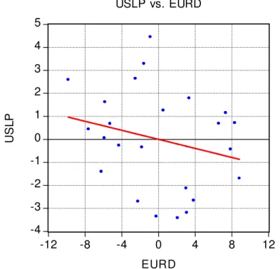
3) The R&D productivity in the EU is found to be a direct Granger-cause of the US total economy labour productivity, and the sign of the relationship is negative. As seen in Figure 6, a negative relationship is also visible in a scatterplot of USLP and EURD.
FIGURE 6. SCATTERPLOT OF LABOUR PRODUCTIVITY IN THE US AND R&D IN THE EU
-4 -3 -2 -1 0 1 2 3 4 5 -12 -8 -4 0 4 8 12 EURD U S L P USLP vs. EURD
This finding relates to the literature on the effects of foreign R&D on domestic productivity. In particular, the negative effect of EURD on USLP is puzzling and it contradicts, for example, the results reported by Coe and Helpman (1995), who argued for positive foreign R&D spillovers on domestic (total factor) productivity. Nevertheless, the results of Coe and Helpman have been weakened by Kao, Chiang, and Chen (1999) who showed that the estimation method of Coe and Helpman contains a bias and the bias-corrected results on the effects of foreign R&D on domestic productivity are rather weak. It should be noted that Coe and Helpman’s estimations cover the period from 1971 to 1990 while we investigate the 1979 – 2002 period. Indeed, an inspection of the Figures 1 and 4
for USLP and EURD suggests the presence of a negative relationship especially in the 1990s. This is consistent with our finding of a negative causal effect from EURD to USRD coupled with a positive reaction of USLP to USRD (e.g. in the 4-variate model). That is, as EURD increases, the USRD decreases, which in turn leads to a decrease in USLP. In view of these findings, the present study adds to the R&D literature by first illustrating the possibility of a negative relationship between foreign R&D and domestic productivity (as in Figure 5) and then presenting causal evidence in favour of it in a multivariate framework. Nevertheless, the effects of R&D activity in the EU on the labour productivity in the US require further research using up-to-date R&D data by source (e.g., public, private, defence) and at the sectoral level.
4) There is no conclusive evidence on direct causality from domestic R&D activity on domestic labour productivity growth. However, a possible indirect effect is still suggested by the finding that USRD does not Granger-cause USLP in the bivariate model but the causal impact of USRD on USLP is positive in the 4-variate model. As a result, the increase in the R&D productivity in the US and the factors driving it might have contributed to the post-1997 increase in the economy-wide labour productivity in the US. In the case of EU, the causal relationships between domestic R&D and labour productivity are rather complex. While there is evidence of a causal link from R&D to labour productivity, the lag structure of this relationship involves both positive and negative coefficients and leads to an overall neutrality result within our sample period. Several explanations for this finding can be offered. First, as Cameron (2005) argues, in a leader-follower game of R&D, the leader-follower may face slower (productivity) growth as it needs to invest into genuine R&D (not just imitation and capital deepening) as the technological distance to the leader narrows. Therefore, a negative relationship between R&D spending and productivity growth might indeed be detected. Hence, our results indicating a complex relationship between the R&D activity and labour productivity in the EU might be partly reflecting the dynamics during the catching-up process. Secondly, the source of R&D is an important consideration. Guellec and Van Pottelsberg de la Potterie (2004), among others, suggest that defense R&D leads to negative spillovers, and the domestic productivity spillovers from business R&D are higher than those of public R&D. Since we use aggregate EU15 R&D data from all sources, our findings might be capturing the possibly differential effects of different R&D-sources on overall productivity. In this context, if achieved, the Lisbon target that two-thirds of the R&D expenditures should be business R&D would help enhance the positive spillovers from R&D activity on the EU’s overall labour productivity. Third, Carlsson and Mudambi (2003) argue that the extent of R&D spillovers on domestic productivity depends on the degree of absorptive capacity, the degree of homogeneity of R&D activity location, and the extent of intra-regional linkages.
Looking at our results in this respect, the aggregate nature of our R&D dataset may again explain the rather unclear findings. For the EU, we use R&D data from 15 countries and the fact is that the distribution of R&D is rather heterogeneous across EU countries. The distribution of the R&D by location is skewed also in the case of the US, possibly limiting the extent of aggregate gains from R&D activity. Overall, our results from aggregate R&D and labour productivity data support the theoretical and institutional arguments that the effects of R&D activity on domestic labour productivity might indeed be ambiguous. While there is some evidence of positive spillovers, the actual dynamics are more complex.
IV. CONCLUSIONS
In this study, we examine the domestic and international linkages among R&D productivity and economy-wide labour productivity in the EU (before the enlargements in 2004 and 2007) and the US using multivariate Granger-causality tests. We find that R&D in the EU is a direct Granger-Hsiao cause of R&D and labour productivity in the US, and the signs of these effects are negative. The EU, on the other hand, shows a positive reaction to the increased R&D productivity in the US and also enjoys positive spillovers from increases in labour productivity in the US. As such, our findings identify the direction of causality in the observed negative correlation between the R&D activity in the EU and the R&D activity in the US. In Scherer’s (1991) terms, the US is found to be responding rather submissively when R&D effort increases in the EU, while EU’s reaction to an increase in R&D efforts by the US is on the aggressive side. The aggressive reaction by the EU reflects itself in different forms, for example, by the gains made in basic research results (e.g., increased share of top 1% publications and citations) even when the R&D activity was stagnating in the EU.
Nevertheless, it should be kept in mind that the findings of this study are based on aggregate R&D data from all sources. There are differences in the composition of R&D between the US and the EU – e.g., the share of public R&D in total R&D expenditures is higher in the EU. Indeed, the EU’s Lisbon targets envisage an increase in the share of private R&D in total R&D expenditures to about 66% from the current levels of about 55%. Therefore, an empirical investigation of whether there is a difference between the responses of public and private R&D in the EU (US) to public and private R&D in the US (EU) remains to be undertaken.
The empirical findings of our study as well as the results of other macro-and micro-level studies in the literature share the view that the US’s R&D reaction to the aggressive R&D efforts by competitors is generally submissive. Hence, if the EU can make progress towards achieving its ambitious R&D targets (possibly at a later date than 2010), the chances of achieving the Lisbon vision
remains good. Still, the achievement of the R&D targets of the Lisbon strategy for the enlarged EU will also depend on the ability of the new member states to spend more financial resources on R&D as well as to change its structure by sources.
APPENDIX
The following is a parameterized application of Hsiao’s (1982) definitions of different types of causal relationships in a 4-variable framework.
GRANGER (NON-) CAUSALITY IN A 4-VARIABLE SYSTEM
∑
∑
∑
∑
= = = − − − = − + + + + + = k i k i k i t i t i i t i i t i k i i t t Y X M Z Y i 1 1 1 1 1 1 1 1 1β
1δ
ϕ
λ
ε
α
∑
∑
∑
∑
= = = − − − = − + + + + + = k i k i k i t i t i i t i i t i k i i t t Y X M Z X i 1 1 1 2 2 2 2 1 2β
2δ
ϕ
λ
ε
α
∑
∑
∑
∑
= = = − − − = − + + + + + = k i k i k i t i t i i t i i t i k i i t t Y X M Z M i 1 1 1 3 3 3 3 1 1β
3δ
ϕ
λ
ε
α
∑
∑
∑
∑
= = = − − − = − + + + + + = k i k i k i t i t i i t i i t i k i i t t Y X M Z Z i 1 1 1 4 4 4 4 1 1β
4δ
ϕ
λ
ε
α
The causal relationship between X and Y can take one of the following forms.
Direct Causality.
a) ∑δ1i ≠ 0, when ∑φ1i ≠ 0 and ∑λ1i ≠ 0; (in a 4-variable system)
b) ∑δ1i ≠ 0, when ∑φ1i ≠ 0 and ∑λ1i = 0; (in a 3-variable system)
c) ∑δ1i ≠ 0, when ∑φ1i = 0 and ∑λ1i ≠ 0; (in a 3-variable system)
d) ∑δ1i ≠ 0, when ∑φ1i = 0 and ∑λ1i = 0; (in a bi-variate system)
That is, X should cause Y in a bivariate system and in all multivariate systems. Direct causality from X to Y is represented as X ⇒ Y.
Feedback. If X ⇒ Y and Y ⇒ X, then there is direct feedback between X and Y.
Or, X ⇔ Y
No Causality.
a) ∑δ1i = 0, when ∑φ1i = 0 and ∑λ1i = 0; (sufficient condition)
b) if ∑δ1i = 0 but ∑φ1i ≠ 0 and ∑λ1i = 0 and if ∑δ3i = 0 in all bi- and multivariate
settings that involve X to explain M,
c) if ∑δ1i = 0 but ∑λ1i ≠ 0 and ∑φ1i = 0 and if ∑δ4i = 0 in all bi- and multivariate
settings that involve X to explain Z,
d) if ∑δ1i = 0 but ∑φ1i ≠ 0 and ∑λ1i ≠ 0 and if ∑δ3i = 0 and ∑δ4i = 0 in all bi-
and multivariate settings that involve X to explain M and Z, then, there is no causality from X to Y (directly or indirectly).
That is, for X not to be a Granger-cause of Y in any way, X should not cause Y directly or indirectly.
Type I Spurious Causality.
If ∑δ1i ≠ 0, when ∑φ1i ≠ 0 and/or ∑λ1i ≠ 0 in a 4- variable system, but ∑δ1i = 0
when ∑φ1i = 0 and/or ∑λ1i = 0 (i.e. in a bi-variate system), then X is said to
cause Y spuriously.
This situation may arise if M and/or Y (together or individually) is/are pre- or co-requires for X to cause Y.
Indirect Causality.
If ∑δ1i = 0 when ∑φ1i ≠ 0 and/or ∑λ1i ≠ 0, but X ⇒ M and / or X ⇒ Z.
Furthermore, ∑δ1i ≠0 when ∑φ1i = 0 and ∑λ1i = 0. Then, X is an indirect, but not
spurious, cause of Y. This case is denoted by X → Y.
In this case, X causes Y via other variables for which it is a direct cause of. Note that the X should cause in a bivariate system or in multivariate systems.
Type II Spurious Causality.
a) the no-causality conditions in (3) hold, except that ∑δ1i ≠0 in a bivariate
b) Furthermore, M ⇒ X and M ⇒ Y and / or Z ⇒ X and Z ⇒ Y. Then, there is Type II spurious causality from X to Y. The case can be similarly derived for Z. This case may arise if, for example, M (Z) is a direct Granger-cause of both X and Y. Then, in the absence of M (Z) (say, in a bivariate causality test between X and Y), X is found to Granger-cause Y, when this result is indeed due to a missing common cause.
REFERENCES
Aghion, Philippe and Howitt, Peter, 1998. Endogenous Growth Theory, The MIT Press, Cambridge, MA.
Bernstein, Jeffrey I., and Mohnen, Pierre, 1998. International R&D Spillovers between U.S. and Japanese R&D Intensive Sectors. Journal of International
Economics 44, 315-338.
Brenner, M. S., and Rushton, M. J., 1989. A Strategic Analysis of Sales Growth and R&D in the Chemical Industry. Research Technology Management March-April, 8-15.
Blonigen, Bruce A., and Slaughter, Matthew J., 2001. Foreign Affiliate and U.S. Skill Upgrading. The Review of Economics and Statistics 83(2), 362-376.
Cameron, Gavin, 2005. The Sun Also Rises: Productivity Convergence Between Japan and the USA. Journal of Economic Growth 10, 387-408.
Carlsson, Bo, and Mudambi, Ram, 2003. Globalisation, Entrpreneurship, and Public Policy: A Systems View. Industry and Innovation 10(1), 103-116.
Chiao, Chaochin, 2001. The Relationship between R&D and Physical Investment of Firms in Science-based Industries. Applied Economics 33, 23-35.
Coe, David T., and Helpman, Elhanan, 1995. International R&D Spillovers.
European Economic Review 39, 859-888.
Coe, David T., Helpman, Elhanan, and Hoffmaister, Alexander, W., 1997. North-South R&D Spillovers. Economic Journal 107, 134-149.
Colombo, Massimo G., and Garrone, Paola, 1996. Technological Cooperative Agreements and Firm’s R&D Intensity. A Note on Causality Relations. Research
Policy 25, 923-932.
Eaton, Jonathan, and Kortum, Samuel, 1996. Trade in Ideas: Patenting and Productivity in the OECD. Journal of International Economics 40, 251-278. Engelbrecht, Hans-Juergen, 1997a. International R&D Spillovers, Human Capital, and Productivity in OECD Countries. European Economic Review 41, 1479-1488. ---, 1997b. International R&D Spillovers among OECD Economies. Applied
Economics Letters 4, 315-319.
Falvey, Rod, Foster, Neil, and Greenaway, David, 2002. North-South Trade, Knowledge Spillovers and Growth. Journal of Economic Integration 17, 650-670. ---, 2004. Imports, Exports, Knowledge Spillovers and Growth. Economics
Letters 85(2), 209-212.
Frantzen, Dirk, (1998) R&D, International Technical Diffusion and Total Factor Productivity. Kyklos 51(4), 489-508.
Garcia-Quevedo, Jose, 2004. Do Public Subsidies Complement Business R&D? A Meta-Analysis of the Econometric Evidence. Kyklos 57(1), 87-102.
Goel, Rajeev K., and Rich, Daniel, P., 2005. Organisation of Markets for Science and Technology. Journal of Institutional and Theoretical Economics 161, 1-17. Granger, Clive W. J., 1969. Investigating Causal Relationships by Econometric Models and Cross-Spectral Methods. Econometrica 36, 424-438
Greunz, Lydia, 2004. Industrial Structure and Innovation – Evidence from European Regions. Journal of Evolutionary Economics 14, 563-592.
Griffith, Rachel, Redding, Stephen, and van Reeten, John, 2004. Mapping the Two Faces of R&D: Productivity Growth in a Panel of OECD Industries. The Review of
Economics and Statistics 86(4), 883-895.
Grilliches, Zvi, 1992. The Search for R&D Spillovers. Scandinavian Journal of
Grossman, Gene M., and Helpman, Elhanan, 1991. Innovation and Growth in the
Global Economy. The MIT Press: Cambridge, MA., USA.
Guellec, Dominique, and van Pottelsberghe de la Potterie, Bruno, 2003. The Impact of Public R&D Expenditure on Business R&D. Economics of Innovation and New
Technology 12(3), 225-243.
---, 2004. From R&D to Productivity Growth: Do the Institutional Settings and the Source of Funds of R&D Matter. Oxford Bulletin of Economics and Statistics 66(3), 353-378.
Hejazi, Walid, and Safarian, Edward, A., 1999. Trade, Foreign Direct Investment, and R&D Spillovers. Journal of International Business Studies 30, 491-511.
Hsiao, Cheng, 1979. Autoregressive Modeling of Canadian Money and Income Data. Journal of the American Statistical Association 74, 553-560.
---, 1982. Autoregressive Modelling and Causal Ordering of Economic Variables.
Journal of Economic Dynamics and Control, 4, 243-259.
Jones, Charles I., 1995. R&D-based Models of Economic Growth. Journal of
Political Economy 103, 759-784.
Kang, Heejon, 1989. The Optimal Lag Selection and Transfer Function Analysis in Granger-Causality Tests. Journal of Economic Dynamics and Control 13, 151-169. Kao, Chicwa, Chiang, Min-Hsien, and Chen, Bangtian, 1999. International R&D Spillovers: An Application of Estimation and Inference in Panel Cointegration.
Oxford Bulletin of Economics and Statistics Special Issue, 691-709.
Kim, J. W., and Lee, H. K, 2004. Embodied and Disembodied International Spillovers of R&D in OECD Manufacturing Industries. Technovation 24, 359-368.
King, David A., 2004. The Scientific Impact of Nations,” Nature 430(15 July), 311-316.
Ko, Kenneth, (2005). The Trade-Off Between R&D and Marketing Spending for High-Technology Companies. The Journal of American Academy of Business 7(1), 59-66.
Kuemmerle, Walter, 1999. The Drivers of Foreign Direct Investment into Research and Development: An Empirical Investigation. Journal of International
Business Studies 30(1), 1-24.
Lewer, Joshua J., and van den Berg, Hendrik, 2003. How Large is International Trade’s Effect on Economic Growth? Journal of Economic Surveys 17(3), 363-396.
Lingens, Joerg, 2005. Policy Implications of Endogenous Growth Models: A Note,” Economics Bulletin, 5(13), 1-7.
Lipsey, Richard G., and Carlaw, Kenneth, I., 2004. Total factor productivity and the measurement of technological change, Canadian Journal of Economics, 37(4), 1118-1150.
Lucas, Robert E., 1988. On the Mechanics of Economic Development. Journal of
Monetary Economics 22, 3-42.
Luintel, Kul B., and Khan, Mosahid, 2004. Are International R&D Spillovers Costly for the United States? The Review of Economics and Statistics 86(4) 896-910.
Neelankavil, James P., and Alaganar, V. T., 2003. Strategic Resource Commitment of High-Technology Firms. An International Comparison. Journal
of Business Research 56, 493-502.
Park, Walter G., 1995. International R&D Spillovers and OECD Economic Growth. Economic Inquiry 33(4), 571-591.
Penm, Jack H. W., and Terrell, Deane, R., 1984. Multivariate Subset Autoregressive Modelling with Zero Constraints for Detecting ‘Overall Causality’. Journal of Econometrics 24, 311-330.
Ravenscraft, David, and Scherer, Frederic M., 1982. The Lag Structure of Returns to Research and Development. Applied Economics 14, 603-620.
Romer, Paul M., 1990. Endogenous Technological Change. Journal of Political
Economy 98(5), S71-S107.
Rouvinen, Petri, 2002. R&D Productivity Dynamics: Causality, Lags, and ‘Dry Holes’. Journal of Applied Economics 5(1), 123-156.
Sargent, Timothy C., and Rodriguez, Edgard, R., 2000. Labour or Total Factor Productivity: Do We Need to Choose? International Productivity Monitor, 1(Fall), 41-44.
Scherer, Frederic M., 1991. International R&D Races: Theory and Evidence. in L. G. Mattsson and B. Stymne (eds.), Corporate and Industry Strategies for Europe. Elsevier Science Publishers B.V.
Schwarz, Gideon, 1978. Estimating the Dimension of a Model. Annal of Statistics 6, 461-464.
Segerstrom, Paul, 1998. Endogenous Growth without Scale Effects. American
Economic Review 88, 1290-1310.
Sturm, Jan-Egbert. and de Haan, Jacob, 1998. Public Capital Spending in the Netherlands: Developments and Explanations. Applied Economics Letters 5(1), 5-10.
Verspagen, Bart, 1995. “R&D and Productivity: A Broad Cross-section Look,”