Weak synchronization and large-scale collective oscillation in dense bacterial suspensions

HAL Id: cea-01483951

https://hal-cea.archives-ouvertes.fr/cea-01483951

Submitted on 8 Mar 2017

HAL is a multi-disciplinary open access

archive for the deposit and dissemination of

sci-entific research documents, whether they are

pub-lished or not. The documents may come from

teaching and research institutions in France or

abroad, or from public or private research centers.

L’archive ouverte pluridisciplinaire HAL, est

destinée au dépôt et à la diffusion de documents

scientifiques de niveau recherche, publiés ou non,

émanant des établissements d’enseignement et de

recherche français ou étrangers, des laboratoires

publics ou privés.

oscillation in dense bacterial suspensions

Chong Chen, Song Liu, Xia-Qing Shi, Hugues Chaté, Yilin Wu

To cite this version:

Chong Chen, Song Liu, Xia-Qing Shi, Hugues Chaté, Yilin Wu. Weak synchronization and

large-scale collective oscillation in dense bacterial suspensions. Nature, Nature Publishing Group, 2017, 542

(7640), pp.210 - 214. �10.1038/nature20817�. �cea-01483951�

2 1 0 | N A T U R E | V O L 5 4 2 | 9 f E b R U A R y 2 0 1 7

LETTER

Weak synchronization and large-scale collective

oscillation in dense bacterial suspensions

Chong Chen1_{*, Song Liu}1_{*, Xia-qing Shi}2_{, Hugues Chaté}3,4 _{& yilin Wu}1

Collective oscillatory behaviour is ubiquitous in nature1_{, having} a vital role in many biological processes from embryogenesis2 and organ development3 _{to pace-making in neuron networks}4_. Elucidating the mechanisms that give rise to synchronization is essential to the understanding of biological self-organization. Collective oscillations in biological multicellular systems often arise from long-range coupling mediated by diffusive chemicals2,5–9_{, by} electrochemical mechanisms4,10_{, or by biomechanical interaction} between cells and their physical environment11_{. In these examples,} the phase of some oscillatory intracellular degree of freedom is synchronized. Here, in contrast, we report the discovery of a weak synchronization mechanism that does not require long-range coupling or inherent oscillation of individual cells. We find that millions of motile cells in dense bacterial suspensions can self-organize into highly robust collective oscillatory motion, while individual cells move in an erratic manner, without obvious periodic motion but with frequent, abrupt and random directional changes. So erratic are individual trajectories that uncovering the collective oscillations of our micrometre-sized cells requires individual velocities to be averaged over tens or hundreds of micrometres. On such large scales, the oscillations appear to be in phase and the mean position of cells typically describes a regular elliptic trajectory. We found that the phase of the oscillations is organized into a centimetre-scale travelling wave. We present a model of noisy self-propelled particles with strictly local interactions that accounts faithfully for our observations, suggesting that self-organized collective oscillatory motion results from spontaneous chiral and rotational symmetry breaking. These findings reveal a previously unseen type of long-range order in active matter systems (those in which energy is spent locally to produce non-random motion)12,13_. This mechanism of collective oscillation may inspire new strategies to control the self-organization of active matter14–18 _{and swarming} robots19_.

Like many other flagellated bacteria, Escherichia coli cells can swarm over the surface of solid substrates such as agar plates20_{, forming}

densely packed colonies with a surface packing fraction21 _{of about 50%.}

Under standard growth conditions (see Methods), E. coli cells (0.8 μ m in diameter, 2–4 μ m in length) produce a 5–10-μ m-thick layer of ‘swarm fluid’22 _{spanning most of the agar surface, in which they swim}

at a mean speed of 34 μ m s−1 _{(Extended Data Fig. 1). The resulting}

quasi-two-dimensional dense bacterial suspension can persist over large spatial scales (centimetres) for hours. We grew about one hundred of such colonies. Approximately 12 h after inoculation, the colony has invaded the whole dish and the cells, observed in phase-contrast videos, display a disordered state with collective motion at small spatial scales (a few tens of micrometres) taking the form of transient jets and vortices (Supplementary Video 1). This ‘bacterial’ or ‘mesoscale’ turbulence has been described recently and the rheology of concentrated suspensions received a lot of attention from active matter physicists23–26_.

As the cell density increases further owing to cell multiplication (Methods), a heretofore unnoticed phenomenon emerges. Although no apparent change seems to occur in phase-contrast videos (Supplementary Video 2), their velocity, measured via particle image velocimetry (PIV) analysis (Methods) and averaged over spatial scales greater than about 100 μ m undergoes regular periodic oscillations within the plane of the swarm-fluid film (Fig. 1c and Extended Data Fig. 2). This collective oscillatory motion (hereafter referred to as ‘collective oscillation’) is characterized by a fluctuating but featureless, spatially homogeneous velocity field that oscillates in time. (Note that this is fundamentally different from the rotational modes or vortical collective motion commonly found in biological and active matter systems under confinement27_{). Once emerged, the collective}

oscillation can persist for at least half an hour. The oscillation period is steady over time and ranges from 4 s to 12 s across different colonies. The orthogonal components of the collective velocity are well fitted by sinusoidal functions with identical period but different amplitude and phase (Extended Data Fig. 2), indicating that the average positions of cells follow elliptical trajectories. We observed the same collective oscillation in swarms of Proteus mirabilis, a species similar to E. coli in terms of motile behaviour but distinct in biochemistry.

The collective oscillation was also clearly manifested when we visua-lized the flow of the upper swarming fluid using silicone-oil droplets with minimal invasiveness (Methods). Strikingly, these tracers followed smooth and oscillatory elliptical trajectories with quasi-synchronized phases even when they were separated by hundreds of micrometres (Fig. 1b and Supplementary Video 2). Their velocity and the collective velocity of cells were in synchrony as well (Fig. 1c), suggesting that the oscillatory flow was generated by the collective motion of cells that drag nearby fluid along28_{. The amplitude of the collective velocity was}

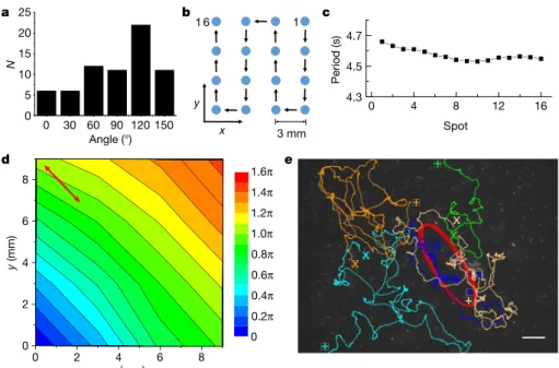
some-what smaller than that of the tracers owing to the averaging procedure. In our experiments we found elliptical collective oscillations most often (68 out of 71 cases), with rare exceptions being linear or irregular oscillations (3 out of 71 cases; Extended Data Fig. 3). In almost all cases, the chirality and the long-axis orientation of collective oscillations are the same within a specific colony, but the chirality has an equal probability of being clockwise or counterclockwise across different colonies (Extended Data Fig. 3a), indicative of spontaneous global chiral symmetry breaking. The long-axis orientation across different colonies is non-uniformly distributed (Fig. 2a), probably reflecting the aniso-tropy of the large-scale geometry of colonies (Extended Data Fig. 1). These results imply that the collective oscillation of cells is correlated over very long distances. To verify this, we measured the period and phase of collective oscillations in an array of spots spanning an area of 9 × 9 mm2 _{(Fig. 2b) (Methods). Remarkably, the period remains}

nearly identical across such a macroscopic area (Fig. 2c), while the phase varies linearly over space (Fig. 2d). The collective oscillation of cells is thus organized over centimetres (more than 104 _{times the cell}

length) in the form of longitudinal travelling waves. In the example 1_{Department of Physics and Shenzhen Research Institute, The Chinese University of Hong Kong, Shatin, Hong Kong, China.} 2_{Center for Soft Condensed Matter Physics and Interdisciplinary} Research, Soochow University, Suzhou 215006, China. 3_{Service de Physique de l’Etat Condensé, CEA, CNRS, Université Paris-Saclay, CEA-Saclay, 91191 Gif-sur-Yvette, France.} 4_Beijing Computational Science Research Center, Beijing 100094, China.

*These authors contributed equally to this work.

9 f E b R U A R y 2 0 1 7 | V O L 5 4 2 | N A T U R E | 2 1 1

given in Fig. 2d, the phase propagated with a wavelength of 17 mm and a phase velocity of 3.7 mm s−1_{. Interestingly, the long axis of collective}

oscillations tends to be perpendicular to the propagation direction of travelling waves.

Next we examined individual trajectories of bacteria within colonies displaying collective oscillation using fluorescent cells (Methods). As suggested by phase-contrast videos (Supplementary Video 2), we found that cells moved erratically without obvious periodic motion but with frequent abrupt turns that are probably due to cell–cell collisions or flagellar switching in a dense environment (Fig. 2e and Supplementary Video 3). Cells also occasionally swam close to the surface and their motion was then weakly biased towards the chirality of the collective oscillation (Extended Data Fig. 4). Sharp turns among different cells were not synchronized, and the time interval between two consecutive turns of the same cell approximately followed an exponential distribu-tion with an average of 2.1 ± 1.9 s (mean ± s.d., n = 118) (Extended Data Fig. 5). This suggests that individual cells do not behave as oscillators, and that the collective oscillation is an emergent weak synchronization phenomenon at the population level, in contrast to most other collec-tive biological oscillations studied2–11_.

We then sought to control the emergence of the collective oscillations. We cooled down entire oscillating colonies to a temperature low enough to suppress any motion of the cells. Coming back then to the original temperature, cells started moving again with normal speed and in random directions (Methods). The collective oscillation typically re-emerged from random motion in about 30 min. At onset an irregular oscillation first emerged spontaneously, then its amplitude increased

and a typical elliptic trajectory was recovered within less than one minute (Fig. 3a, c and Extended Data Fig. 6a, b). Remarkably, the long-axis orientation and the chirality were uncorrelated to the original one. These results confirm that collective oscillation is the result of spontaneous symmetry breaking. In fact, we also found that collective oscillation in cooled-off colonies may re-emerge simultaneously in several regions with different chirality and we observed that the inter-face separating two adjacent regions with collective oscillations of opposite chirality moves, resulting in local chirality switching accom-panied by a gradual change of the orientation of the ellipses (Fig. 3b, d and Extended Data Fig. 6c, d). This observation suggests that travelling waves seen in naturally developed colonies may result from the com-petition of collective oscillations having emerged in different domains and are not strongly coupled with colony development.

Finally, we investigated the mechanism driving collective oscillations. We optically deactivated the motility of cells in a small area of colonies already displaying collective oscillation (Methods; Extended Data Fig. 7 and Supplementary Video 4). We found that as the speed of the cells decreased, the amplitude of collective oscillation, as measured by the collective cell velocity and by tracer velocity, decreased as well and eventually almost vanished when all cells became totally immotile, with a small-amplitude residual oscillation reflecting the incompressibility of fluids (Extended Data Fig. 7b). On the other hand, the collective oscilla-tion remained unchanged beyond about 50 μ m outside the boundary of the motility-deactivated area (Extended Data Fig. 7c, d). These results confirm that cell motility provides the driving force of collective oscillation, and that the mechanism maintaining this emergent phenomenon is local in nature and highly robust to perturbation.

We now present a mathematical model at the individual, ‘particle’ level that accounts for all our experimental observations. (We note that our model cannot be fully conclusive at this stage because it is based on assumptions that will need to be confirmed by a detailed study of the complex interactions between bacteria bodies, flagella, gel substrate, and the surrounding fluid.) First, in a minimalist approach, we consider identical self-propelled particles with strictly local interactions, without modelling the surrounding fluid explicitly. Second, to account for the experimental observations left unexplained, we ‘immerse’ this model in some Stokesian incompressible fluid.

In the Vicsek-style16,29_{, ‘dry’ core of our model, point particles move}

at constant speed v0 in a two-dimensional domain without any repulsive

or attractive interaction. This allows us (1) to account for the fact that in the experimental swarming fluid layer cells can pass above each other, and (2) to simulate easily millions of cells, as required by the large-scale, high-density context of the phenomena observed. Single-particle dynamics involves an evolution equation for the velocity direction θ that allows for local alignment, but also one for the angular velocity or instantaneous frequency ω θ=  to account for short-time memory effects introduced by the local fluid vorticity and to allow for synchronization of local rotational motion. Both these equations are stochastic, with strong noise guaranteeing erratic individual trajectories. Particles within a distance d0 of the order of the bacteria

body length are subjected to two interactions, a diffusive coupling between angular velocities of strength kω, and a polar alignment of

strength kθ:

∑

∑

where the sums are over the ni particles j currently in the

neighbour-hood of i, and the delta-correlated noises ξθ and ξω are drawn from

symmetric uniform distributions in the intervals [−η η_θ, ]_θ and

η η

− _{ω ω}

[ , ]. On the other hand, ξbias has the (current) sign of ω and its a c b x y 0 5 10 15 20 25 30 –20 –10 0 10 20 v (μ m s –1) Time (s)

Figure 1 | Collective oscillation in dense suspensions of E. coli. a, Representative velocity field of cells’ collective motion obtained by PIV

analysis (see Methods). The red arrow indicates the direction of average velocity. In all experimental figures throughout the paper, the + x axis represents the colony expansion direction (Extended Data Fig. 1). b, In the same field of view as a, two silicone oil tracers (red dots) displayed synchronized oscillation in elliptical trajectories (Supplementary Video 2). The background is the first frame of Supplementary Video 2. Scale bars in

a and b are 20 μ m. c, Cells’ collective velocity (blue, x-axis component; red, y-axis component) and tracer velocity (green, x-axis component; black, y-axis component) in Supplementary Video 2 plotted against time.

2 1 2 | N A T U R E | V O L 5 4 2 | 9 f E b R U A R y 2 0 1 7 x y 3 mm 1 1 6 b 0 30 60 90 120 150 0 5 10 15 20 25 N Angle (°) a d 1.6π 0.2π 0.4π 0.6π 0.8π 1.0π 1.2π 1.4π 0 6 4 2 0 0 2 4 6 y (mm) x (mm) 8 8 Period (s) Spot 0 4 8 12 16 4.3 4.5 4.7 c e

Figure 2 | Collective oscillation organized into a centimetre-scale travelling wave. a, Distribution of long-axis orientation of collective

oscillations (that is, the angle defined in Extended Data Fig. 1b) across N = 71 colonies. b, Sequence of measuring a 4 × 4 array of spots on a colony undergoing collective oscillation (Methods). c, The period of collective oscillation at all spots plotted in the order of measurement.

d, Contour map of the phase distribution of collective oscillation across

the same colony as in c. The phase (colour scale, in radians) can be fitted

as ϕ = 0.25x + 0.27y (Methods), propagating at 0.37 rad mm−1 _{along its} gradient direction. The double-ended red arrow indicates the long axis of collective oscillation. e, Single-cell trajectories in the mid-layer during collective oscillation (crosses, starting points; pluses, ending points; see Supplementary Video 3). An immotile cellular cluster (red trajectory) can serve as a flow tracer. Scale bar, 20 μ m. The background is the last frame of Supplementary Video 3. a c x (μm) x (μm) –30 –20 –10 0 y (μ m) y (μ m) –10 0 10 20 30 40 Time (s) Time (s) d b 100 50 0 150 0 50 100 150 –30 –20 –10 0 40 30 20 10 0 Time (s) Time (s) 0 50 100 150 –20 –10 0 10 20 Velocity (μ m s –1) Velocity (μ m s –1) 0 50 100 150 –10 –5 0 5 10 200 Figure 3 | Emergence of collective oscillation and chirality switching.

a, Collective trajectory of cells during the emergence of collective

oscillation. b, Chirality switching of collective oscillation from counterclockwise to clockwise during domain competition. Trajectories

in a and b were built from the collective cellular velocity obtained by PIV analysis (the colour scale shows time in seconds). c, d, Collective velocities associated with a and b fitted by the smoothing spline method based on PIV data (red, x-axis component; black, y-axis component) (see Methods).

9 f E b R U A R y 2 0 1 7 | V O L 5 4 2 | N A T U R E | 2 1 3

amplitude decreases with ω: ξbias=_{sign( )exp(}ωi −ω ω ξi/ 0₎ where ξ

is a uniform noise in [0,ηbias]. This ‘bias’ noise, together with the

diffusive coupling between angular velocities, gives the possibility of chiral symmetry-breaking leading to a spatially homogeneous and globally oscillating velocity field. Simulations of equations (1) to (2) showed that there is a large region of parameter space where collective oscillatory motion emerges: global angular velocity Ω= ω and global polarity P= exp( )iθ take finite values while individual trajectories remain erratic (Fig. 4a, b; Methods). Not surprisingly for a diffusive oscillatory medium30_{, travelling-wave configurations with arbitrary}

large wavelength are stable. However, as indicated by the constancy over time of Ω and P, average trajectories remain roughly circular in all cases (Fig. 4a, b), in contrast to experimental observations.

We now take into account the surrounding viscous fluid in a simpli-fied way (see Methods for a more complete presentation). Cells interact with the surface of the agar gel, pushing themselves away from it and entraining some fluid with them. The incompressible, damped fluid is governed by a Stokes equation, creating a flow field v that advects particles:

Simulations of this suspension model show that, in travelling-wave configurations, average trajectories of particles are ellipses with the long axis perpendicular to the wave propagation direction, in agreement with experimental observations (Fig. 4c–e and Fig. 2d). The model also accounts well for the residual collective oscillations seen in motility- deactivation experiments (Extended Data Fig. 8 and Supplementary Video 8).

Taking all results together, we conclude that the emergence of collective oscillatory motion in swarming flagellated bacteria is a robust self- organized process probably mediated by local interactions. A defining feature of this process is that individual cells remain strongly erratic while global order emerges. In contrast to other collective biological oscillations studied so far2–11_{, which mostly arise from phase- coupling}

between explicit local oscillators, the phenomenon we report is characterized by two key factors. First, our system does not have ‘obvious’ local oscillators—they emerge only from noise upon sufficient coarse- graining; second, our synchronization is of erratic trajectories, that is, it occurs in physical space but not in phase space. As such, this phenomenon may constitute weak synchronization of stochastic

trajectories, a type of ordered active matter not seen before, to our knowledge. The phenomenon may influence spatial patterning of biofilms in bacterial colonies (Extended Data Fig. 9). This mechanism of collective oscillation may be relevant to diverse biological processes that involve a large population of locally interacting cells with noisy and non-oscillating individual behaviour.

Online Content Methods, along with any additional Extended Data display items and

Source Data, are available in the online version of the paper; references unique to these sections appear only in the online paper.

received 12 June; accepted 1 November 2016. Published online 23 January 2017.

1. Winfree, A. T. The Geometry of Biological Time (Springer, 1980). 2. Oates, A. C., Morelli, L. G. & Ares, S. Patterning embryos with oscillations:

structure, function and dynamics of the vertebrate segmentation clock.

Development 139, 625–639 (2012).

3. He, L., Wang, X., Tang, H. L. & Montell, D. J. Tissue elongation requires oscillating contractions of a basal actomyosin network. Nat. Cell Biol. 12, 1133–1142 (2010).

4. Herzog, E. D. Neurons and networks in daily rhythms. Nat. Rev. Neurosci. 8, 790–802 (2007).

5. Muller, P. et al. Differential diffusivity of Nodal and Lefty underlies a reaction-diffusion patterning system. Science 336, 721–724 (2012).

6. Gregor, T., Fujimoto, K., Masaki, N. & Sawai, S. The onset of collective behavior in social amoebae. Science 328, 1021–1025 (2010).

7. Danino, T., Mondragon-Palomino, O., Tsimring, L. & Hasty, J. A synchronized quorum of genetic clocks. Nature 463, 326–330 (2010).

8. Liu, J. et al. Metabolic co-dependence gives rise to collective oscillations within biofilms. Nature 523, 550–554 (2015).

9. De Monte, S. et al. Dynamical quorum sensing: population density encoded in cellular dynamics. Proc. Natl Acad. Sci. USA 104, 18377–18381 (2007). 10. Bennett, M. V. L. & Zukin, R. S. Electrical coupling and neuronal

synchronization in the mammalian brain. Neuron 41, 495–511 (2004). 11. Koride, S. et al. Mechanochemical regulation of oscillatory follicle cell dynamics

in the developing Drosophila egg chamber. Mol. Biol. Cell 25, 3709–3716 (2014).

12. Ramaswamy, S. The mechanics and statistics of active matter. Annu. Rev.

Condens. Matter Phys. 1, 323–345 (2010).

13. Marchetti, M. C. et al. Hydrodynamics of soft active matter. Rev. Mod. Phys. 85, 1143–1189 (2013).

14. Nédélec, F. J., Surrey, T., Maggs, A. C. & Leibler, S. Self-organization of microtubules and motors. Nature 389, 305–308 (1997).

15. Schaller, V., Weber, C., Semmrich, C., Frey, E. & Bausch, A. R. Polar patterns of driven filaments. Nature 467, 73–77 (2010).

0 50 100 150 200 250 0 0.2 0.4 0.6 0.8 Ω 0 50 100 150 200 250 0 0.1 0.2 0.3 0.4 0 50 100 150 –12 –6 0 6 12 Global frequency, Global polarity, P Time (s) Time (s) V_x V_y Vx , Vy (μ m s –1) Time (s) 20 μm 100 μm a b c d e 16 12 8 4 0 y (μ m) 1,200 900 600 300 0 0 5 10 15 20 Time (s) 2π π 0 3π/2 π/2

Figure 4 | Modelling results. a, Snapshot of ‘dry’ self-propelled particle

model in a homogeneous, counterclockwise collective oscillation regime (Supplementary Video 5). Trajectories of randomly selected particles were shown during two periods of the collective oscillation cycle (start, blue; end, red). The line at the bottom left is a collective trajectory built from the averaged velocity of all particles (about 20,000). b, Time series of global frequency Ω, global polarity P, and collective velocity components Vx (horizontal) and Vy (vertical) from random initial conditions (same parameters as in a). c, Snapshot of the ‘wet’ model in a stationary travelling

wave regime, with particles coloured by their orientation θ (angular colour scale on the right of e) (Supplementary Video 6). The inset shows the zoom of the elliptical trajectory built from the averaged velocity of particles in a 96 μ m × 96 μ m local domain. d, Fluid flow corresponding to c (Supplementary Video 7). The colour scale shows the intensity of the local fluid speed (in micrometres per second). e, Spatiotemporal dynamics of the oscillation phase of Vx(y, t) showing the propagation of the travelling wave (angular colour scale).

2 1 4 | N A T U R E | V O L 5 4 2 | 9 f E b R U A R y 2 0 1 7

16. Sumino, Y. et al. Large-scale vortex lattice emerging from collectively moving microtubules. Nature 483, 448–452 (2012).

17. Sanchez, T., Chen, D. T. N., DeCamp, S. J., Heymann, M. & Dogic, Z. Spontaneous motion in hierarchically assembled active matter. Nature 491, 431–434 (2012).

18. Bricard, A., Caussin, J.-B., Desreumaux, N., Dauchot, O. & Bartolo, D. Emergence of macroscopic directed motion in populations of motile colloids.

Nature 503, 95–98 (2013).

19. Rubenstein, M., Cornejo, A. & Nagpal, R. Programmable self-assembly in a thousand-robot swarm. Science 345, 795–799 (2014).

20. Kearns, D. B. A field guide to bacterial swarming motility. Nat. Rev. Microbiol. 8, 634–644 (2010).

21. Darnton, N. C., Turner, L., Rojevsky, S. & Berg, H. C. Dynamics of bacterial swarming. Biophys. J. 98, 2082–2090 (2010).

22. Wu, Y. & Berg, H. C. A water reservoir maintained by cell growth fuels the spreading of a bacterial swarm. Proc. Natl Acad. Sci. USA 109, 4128–4133 (2012).

23. Zhang, H. P., Be’er, A., Smith, R. S., Florin, E.-L. & Swinney, H. L. Swarming dynamics in bacterial colonies. Europhys. Lett. 87, 48011 (2009).

24. Sokolov, A. & Aranson, I. S. Physical properties of collective motion in suspensions of bacteria. Phys. Rev. Lett. 109, 248109 (2012).

25. Wensink, H. H. et al. Meso-scale turbulence in living fluids. Proc. Natl Acad.

Sci. USA 109, 14308–14313 (2012).

26. López, H. M., Gachelin, J., Douarche, C., Auradou, H. & Clément, E. Turning bacteria suspensions into superfluids. Phys. Rev. Lett. 115, 028301 (2015).

27. Lushi, E., Wioland, H. & Goldstein, R. E. Fluid flows created by swimming bacteria drive self-organization in confined suspensions. Proc. Natl Acad.

Sci. USA 111, 9733–9738 (2014).

28. Pushkin, D. O., Shum, H. & Yeomans, J. M. Fluid transport by individual microswimmers. J. Fluid Mech. 726, 5–25 (2013).

Supplementary Information is available in the online version of the paper. Acknowledgements We thank Y. Li and W. Zuo from our laboratory for building

the microscope stage temperature control system, L. Xu (The Chinese University of Hong Kong) for providing silicone oil, H. C. Berg (Harvard University) for providing the bacterial strains, and J. Näsvall and J. Bergman (Uppsala University) for providing the mRFP plasmid. This work was supported by the Research Grants Council of Hong Kong SAR (RGC numbers 2191031 and 2130439 and CUHK Direct Grant numbers 3132738 and 3132739 to Y.W.), the National Natural Science Foundation of China (NSFC number 21473152, to Y.W.; NSFC number 11635002 to H.C. and X.S.; NSFC numbers 11474210, 11674236 and 91427302 to X.S.), and the Agence Nationale de la Recherche (project Bactterns, to H.C.).

Author Contributions Y.W. discovered the phenomenon and designed the study.

C.C. and S.L. performed experiments. C.C., S.L., Y.W. analysed and interpreted the data, with input from H.C. X.S. and H.C. developed the mathematical model. All authors wrote the paper.

Author Information Reprints and permissions information is available

at www.nature.com/reprints. The authors declare no competing

financial interests. Readers are welcome to comment on the online version of the paper. Correspondence and requests for materials should be addressed to Y.W. (ylwu@phy.cuhk.edu.hk), H.C. (hugues.chate@cea.fr) or X.S. (xqshi@suda.edu.cn).

reviewer Information Nature thanks J. Hasty and the other anonymous

reviewer(s) for their contribution to the peer review of this work.

29. Vicsek, T. et al. Novel type phase transition in a system of self-driven particles.

Phys. Rev. Lett. 75, 1226–1229 (1995).

30. Kuramoto, Y. Chemical Oscillations, Waves, and Turbulence (Springer, 1984).

MethOdS

No statistical methods were used to predetermine sample size.

Bacterial strains. The E. coli stains used in this study were HCB1737 (a derivative

of wild- type E.coli AW405 with FliC S219C mutation; a gift from Howard C. Berg, Harvard University) and HCB1737 expressing monomeric red fluorescent protein (mRFP) (HCB1737 transformed with an L-arabinose inducible mRFP plasmid provided by J. Näsvall, Uppsala University). Single-colony isolates were grown overnight with shaking in LB medium (1% Bacto tryptone, 0.5% yeast extract, 0.5% NaCl) at 30 °C to stationary phase. For HCB1737 mRFP, kanamycin (50 μ g ml−1₎ was added to the growth medium. Overnight cultures were diluted 1/100 for inoculating swarm plates. For single-cell tracking, overnight cultures of HCB1737 mRFP were mixed with HCB1737 at 1% and the mixture was diluted 1/100 for inoculating swarm plates.

Swarm plates. Swarm agar (0.6% Eiken agar infused with 1% Bacto peptone, 0.3%

beef extract, and 0.5% NaCl) was autoclaved and stored at room temperature31_. Before use, the agar was melted in a microwave oven, cooled to 60 °C, and pipetted in 13-ml aliquots into 90-mm polystyrene Petri plates. Taking the shear modulus of 0.6% agar as approximately 4.5 kPa (ref. 32), the oscillation frequency of the approximately 2-mm-thick agar substrate in our preparations is about 240 Hz, so the oscillation of the agar substrate would be irrelevant to the collective oscillation we report (< 1 Hz). For optical deactivation of cell motility, the dye FM4-64 (Life Technologies) was dissolved in deionized water and added at a final concentration of 1.0 μ g ml−1 _{to the liquefied swarm agar before pipetting. For single-cell tracking} with HCB1737 mRFP cells, the inducer L-arabinose was added to the swarm agar at 0.02% (wt/vol) before pipetting. The plates were swirled gently to ensure surface flatness, and then cooled for 5 min without a lid inside a large Plexiglas box. Drops of diluted overnight bacterial cultures (1 μ l; described above) were inoculated at a distance of 1 cm from the edge of the plates. The plates were dried for another 10 min without a lid, covered, and incubated overnight at 30 °C and about 95% relative humidity for 18–19 h to observe collective oscillation in the colonies. During swarming the colonies are covered by a self-maintained, micrometres-thick layer of fluid (that is, the swarm-fluid film; see Extended Data Fig. 1).

The development of a typical swarming colony in our experimental conditions proceeded as follows. Within about 5 h after inoculation, cells were adapting the surface growth environment and producing the swarm-liquid film, and there was little colony expansion; this stage is referred to as the lag phase. After the lag phase, the colony (as well as the swarm-fluid film) started advancing at a speed of around 1–1.5 cm h−1_{, until the entire agar surface was covered at about 12 h after} inoculation. Cells then continued to grow and remained motile, and the swarm-fluid film became thicker. Collective oscillation typically appeared at about 18–19 h after inoculation, presumably when cell density reaches above 5 × 1010 _ml−1 _or about 20% volume fraction (Extended Data Fig. 10). In the meantime, cells at the inoculum gradually became sessile and formed biofilms owing to nutrient depletion. Biofilm formation spread to nearly the entire colony at about 24 h after inoculation.

Preparation of silicone oil tracers. Surfactant Tween 20 (Sigma) was mixed with

silicone oil (viscosity 0.65 mPa s, specific gravity 0.76; Shin-Etsu, KF-96L-0.65CS) at a final concentration of 50 mg l−1 _{and stored in a sprayer. Prior to observation,} the silicone oil was sprayed gently over the colony surface, producing silicone oil droplets with a diameter of about 2–6 μ m that fall onto the swarm fluid at random positions. Tween 20 helps silicone oil droplets to penetrate the surfactant layer covering the swarm fluid film33_{. The silicone oil droplets (with a density smaller} than water) appeared to stay in the upper portion of the swarm-fluid film because cells tended to pass by underneath without colliding with them. This method is a minimally invasive way to introduce tracers into the swarm-fluid film and does not disturb the collective motion of cells in the colony.

Cooling-off cell motility in the entire colony. E. coli swarm colonies grown for

about 18 h as described above (that is, at the early stage of collective oscillation) were placed in a 4 °C refrigerator for around 20 min, and then moved onto a micro-scope stage maintained at 30 °C for observation. The motility of cells in the entire colony ceases during refrigeration. Once the colony is brought back from 4 °C up to 30 °C, random collective motion appears after about 20 min as cell motility recovers, and collective oscillation typically re-emerges in another 30 min or so.

Imaging cells and optical deactivation of cell motility. Collective motion of cells

was observed in phase contrast with a 40 ×  objective (Nikon CFI Plan Fluor DLL 40× , numerical aperture 0.75, working distance 0.66 mm) mounted on an upright microscope (Nikon Ni-E). For single-cell tracking, HCB1737 mRFP cells were imaged in epifluorescence using the 40 ×  objective and an mCherry filter cube (excitation 562/40 nm, emission 641/75 nm, dichroic 593 nm; mCherry-B-000, Semrock Inc.), with the excitation light provided by a mercury precentred fibre illuminator (Nikon Intensilight). To measure the period and phase distribution of collective oscillation in a colony, a 16-min phase-contrast video was taken at 16 spots in total (forming a 4 × 4 array with a separation of 3 mm between

neighbouring spots), with an observation time of 50 s at each spot and 10 s for switching to the next spot in the specified sequence using the motorized micro-scope stage controlled by NIS Elements software (Nikon). For optical deactivation of cell motility during collective oscillation using the photosensitizing effect of the membrane dye FM4-64, part of the field of view (about 160 μ m in diameter) was illuminated by orange-red light (from Nikon Intensilight) passing through a 562/40 nm filter (FF01-562/40-25, Semrock Inc.) to excite FM4-64. Upon excitation, FM4-64 disrupts flagellar motility (Extended Data Fig. 7a), most probably owing to the release of reactive oxygen species, similar to other photosensitizing dyes34_{. Recordings were made with a sCMOS camera (Andor Neo} 5.5) at 30 fps operating in global-shutter mode. In all experiments the Petri dishes were covered with a lid to prevent evaporation and air convection, and the sample temperature was maintained at 30 °C using a custom-built temperature control system installed on microscope stage.

Image processing and data analysis. The velocity field of cells’ collective motion

was obtained by performing PIV analysis on microscopy videos using an open-source package MatPIV 1.6.1 written by J. Kristian Sveen (http://folk.uio.no/jks/ matpiv/index2.html). For each pair of consecutive images, the interrogation- window size started at 20.8 μ m × 20.8 μ m and ended at 5.2 μ m × 5.2 μ m after six iterations. The grid size of the resulting velocity field was 2.6 μ m × 2.6 μ m. Silicone-oil tracers were tracked in phase-contrast videos using a custom- written particle-tracking program in MATLAB (The MathWorks, Inc.), and tracer velocities were computed from the tracking data. Collective velocity was obtained by averaging the PIV velocity field. Collective velocity components in Fig. 3c and d and Extended Data Fig. 6d were fitted by the smoothing spline method in MATLAB. Fluorescent HCB1737 mRFP cells were tracked manually using the MTrackJ plugin (E. Meijering, http://www.imagescience.org/meijering/software/ mtrackj/) developed for ImageJ (http://rsbweb.nih.gov/ij/). In the case of collective oscillation, the components of tracer velocity and of the collective velocity of cells were fitted as sinusoidal functions of time using the least-squares method in MATLAB in the following form: v(t) = a1sin(2π t/a2 + a3) + a4, where a1, a2, a3 and a4 are fitting parameters that represent the amplitude, period, phase constant, and drift constant of the velocity components. The long-axis orientation of tracer trajectories was measured manually in ImageJ. The contour maps of phase distri-bution across space were plotted and fitted with Origin 9 (OriginLab Corporation).

‘Dry’ and ‘wet’ mathematical models of collective oscillations. The

Vicsek-style, ‘dry’ core of our model, is similar to the model developed to account for the collective behaviour of microtubules displaced by a carpet of motor proteins16,35_. Point particles move at constant speed v0 in a two-dimensional domain without any repulsive or attractive interaction. Single-particle dynamics is governed by two stochastic equations, with strong noise guaranteeing erratic individual trajectories. A major difference from the models of refs 16 and 35 is that particles are subjected to two interactions, a diffusive coupling between angular velocities and a polar alignment interaction as described in the main text (see equations (1) and (2)). For simplicity the interaction neighbourhood is a disk of radius of the order of the bacteria body length.

Simulations of equations (1) and (2) were performed at the relatively high global density ρ0 = 5 roughly corresponding to the experimental conditions. The simulation domain shown in Fig. 4a is a 64 × 64 square containing approximately 20,000 particles, in which no large-scale spatial structure is apparent. Other parameter values in simulations of this ‘dry’ model: kθ = 0.4, kω = 2, ηθ = 1, ηω = 0.2,

ηbias = 1, ω0 = 0.05, τ = 1 and v0 = 1. As seen in Fig. 4b, synchronization of

instan-taneous frequencies arises first (chirality symmetry breaking), followed in time by phase synchronization (orientational order/rotational symmetry breaking). The model also supports travelling-wave solutions of wavenumber q∈[0,q_max]. In the homogeneous oscillation regime (q = 0), as well as in travelling-wave configura-tions (q ≠ 0), the collective trajectory is roughly circular.

Our ‘wet’ model produces elliptic trajectories in the travelling-wave regime. It takes into account the surrounding viscous fluid in a simplified way. Everything remains in two space dimensions. Cells frequently interact with the gel at the bottom, pushing themselves away from it and entraining some fluid with them. This creates a flow field v(r) that advects particles: r vi= +v0uˆi where uˆi is the unit

vector of orientation θi.

All flows take place in the viscous regime at very low Reynolds number, and the response of the fluids to the internal drive exerted by bacteria is fast enough that we can use the Stokes equations to describe the quasi-steady-state of the fluid. To obtain the simple Stokes equation with entraining forces and proper incompressibility condition, we first consider a two-fluid-layer model where the bacteria’s action on the total fluid conserves momentum. The flow in the upper layer, containing the swarming bacteria, is described by v(r), and vs(r) is the flow in the bottom gel near its surface. During the entraining process, bacteria exert a force field F(r) upon the upper layer of the fluid, and at the same time ‘kick’ the fluids near the substrate with − F(r), so that the total momentum during this

process is conserved. The microscopic mechanism for such kicking dynamics is not clear in such a dense ‘glue’ of bacteria bodies entangled in flagellar filaments near the porous substrate. However, as we will show below, it is enough to support the entraining flow found by experiment. The Stokes equations governing these processes are given by:

µ∇ + ∇ −2v P α0(v v− s)−γ1v F+ =0 (3) µ_s∇2v_s+ ∇ −P α_{0 s}(v v− )−γv F− =0 (4) 2 s λ λ ⋅ ∇[ v+ s sv] 0= (5)

where μ and μs are the effective viscosity of the upper layer and substrate layer, and α0 is the effective friction coefficient between these two layers of the fluids. The pressure P enforces the incompressibility condition. It is the same for both layers because there is no exchange of fluids between these two layers when the quasi-steady state is reached. The friction coefficient on the fluid at the air-water interface is γ1 and γ2 is the friction between the gel and the swarming fluid. The incompressibility condition is applied for the total two layers of fluids, and λ/λs describes the effective local mass ratio between the two layers. The entraining force field F(r) is assumed to be proportional to the local polarity of bacteria:

δ

= ∑ −

F r( ) k _{i i}uˆ r r( i) where uˆi is the unit vector in the direction of θi. These equations can be simplified if we consider that the fluid motion vs(r) near and inside the gel is highly damped by a large coefficient γ2. Then the friction term becomes dominant in equation (4). At large scales, neglecting the contribution from terms with spatial derivatives, we can obtain vs=(α0v F− /) (α0+γ2).

Inserting this into equations (3) and (5), we obtain:

µ∇ + ∇ −2v P αv f 0+ = (6)

β ⋅

∇(v− f) 0= (7)

where α α γ α= 0 2/( 0+γ2)+γ1 is an effective friction coefficient,

κ

γ α γ δ

= / + = ∑ −

f 2F ( 0 2) _{i i}uˆ r r( i), κ γ= 2k (/α0+γ2) is the effective

entrain-ment strength, and β λ α= s( 0+γ2) [ (/λ α0+γ2)+α λ γ0 s 2] is the effective

mobility coefficient of the backflow upon the reaction of f.

Simulations. To numerically solve equations (6) and (7), we first construct the

force field f from the off-lattice particle positions and orientations. There are various ways to construct f. Here we use a simple and efficient one: we divide the system into a lattice of unit length boxes, and perform the summation over particles in each box. The flow velocity field v and pressure field P are then computed on the same lattice. They are solved first in Fourier space and then transformed back into real space.

Parameter values for the simulations of the ‘wet’ model shown in Fig. 4c–e are the same as for the dry model simulations in Fig. 4a and b and μ = 2, α = 10, β = 0.2 and κ = 2. The simulation domain shown in Fig. 4c and d is a 512 × 64 rectangular domain containing about 163,000 particles. To obtain the spatiotemporal dynamics of the phase of collection oscillations shown in Fig. 4e, the phase of collection oscillations ϕ(y, t) was determined by fitting Vx(y, t) (that is, the horizontal component of collective cell velocity obtained by averaging over 32 × 32 domains at different y-positions for simulations associated with Fig. 4c and d) using

ϕ

+

V y0( )cos(wt 0( ))y , and ϕ( , )y t =wt+ϕ0( )y shows the propagation of the

travelling wave. To convert numbers in both ‘dry’ and ‘wet’ model simulations to physical units, we set unit length in the model as 3 μ m (that is, about one cell length), and set particle speed as 30 μ m s−1_{. So the particle density ρ0 = 5 we chose} corresponds to 5 cells per 9 μ m2_.

Data availability. The authors declare that all data generated during this study

are included in the paper. The raw images and videos that support the findings of this study are available from the corresponding author upon reasonable request.

31. Turner, L., Zhang, R., Darnton, N. C. & Berg, H. C. Visualization of flagella during bacterial swarming. J. Bacteriol. 192, 3259–3267 (2010).

32. Hamhaber, U., Grieshaber, F. A., Nagel, J. H. & Klose, U. Comparison of quantitative shear wave MR-elastography with mechanical compression tests.

Magn. Reson. Med. 49, 71–77 (2003).

33. Zhang, R., Turner, L. & Berg, H. C. The upper surface of an Escherichia coli swarm is stationary. Proc. Natl Acad. Sci. USA 107, 288–290 (2010). 34. Spikes, J. D. in The Science of Photobiology (ed. Smith, K. C.) 79–110 (Springer,

1989).

35. Nagai, K. H., Sumino, Y., Montagne, R., Aranson, I. S. & Chaté, H. Collective motion of self-propelled particles with memory. Phys. Rev. Lett. 114, 168001 (2015).

36. Chaté, H., Grinstein, G. & Tang, L. H. Long-range correlations in systems with coherent (quasi)periodic oscillations. Phys. Rev. Lett. 74, 912 (1995).

Extended Data Figure 1 | Illustration of a swarming colony. a, Top view

of the colony. E. coli cells were inoculated near the edge of the Petri dish (grey dot) to initiate swarming (Methods). The arrow indicates colony expansion direction before the colony covers the entire Petri dish (9 cm in diameter). At the time of observing collective oscillations in the colony, the colony has covered the entire available surface on the Petri dish and ceased expansion. Cells within 1–2 cm of the inoculum have already become sessile and turned into biofilm, while most cells in the area enclosed by the red line remain motile. Once emerged, collective oscillations span over the entire area enclosed by the red line. In the specified x–y coordinate system, the + x axis represents the colony expansion direction. b, Illustration of the average position of cells undergoing collective oscillation in the form of elliptical trajectories. The blue line indicates the long-axis orientation

of the elliptical trajectory (that is, the orientation along which collective osillcations have the greatest amplitude), and θ denotes the angle between the long axis and the x axis in a. The distribution of θ across different colonies is given in Fig. 2a. It tends to be along the y-axis, that is, perpendicular to the colony-expanding direction. Colonies are typically more isotropic along the y-axis. So the result in Fig. 2a suggests that the development of collective oscillations is influenced by the large-scale anisotropy of the system. c, Side view of the colony. The swarming colony establishes a swarm-fluid film of thickness 5–10 μ m in which a dense population of cells is dispersed. The top surface of the swarm-fluid film is in contact with air and covered by a monolayer of surfactant (see ref. 33), and the bottom surface is in contact with agar.

Extended Data Figure 2 | Collective velocity of cells undergoes periodic oscillation. a, Components of cells’ collective velocity obtained by PIV

analysis (green, x-axis component; black, y-axis component; same data as in Fig. 1c) were fitted by the following sinusoidal functions: vx = 6.25 × sin(0.95t + 0.66) + 0.01 μ m s−1_{, and vy = 11.9 × sin(0.95t −  1.49) μ m s}−1_. b, Temporal correlation of collective velocity. The temporal correlation was

first calculated for each grid of the velocity field obtained by PIV analysis and then averaged over the entire velocity field, using the following formula:

⋅

∆ = V r V r + ∆ / V r V r + ∆

C t( ) ( , ) ( ,t t t) ( ( , ) ( ,t t t) )t,r, where V(r, t)

denotes the velocity vector in a grid located at position r and at time t, and the angular brackets denote averaging first over time t and then over all grids. The grey area represents standard error of the mean when averaging over all grids. c, Temporal evolution of collective velocity. This figure plots collective velocities average over an area of L × L and connects them in the order of time. Three window sizes (L) for averaging are chosen: 19.5 μ m

(black), 59.8 μ m (red), and 100.1 μ m (blue). Apparently collective velocity measured over larger areas tends to fluctuate less and better reveals the oscillatory nature of the collective velocity field. This is similar to what can be measured in ‘non-trivial collective behaviour’ in cellular automata and other dynamical systems; see ref. 36 and references therein. d, Speed fluctuation versus averaging window size. The normalized fluctuation (or fluctuation-speed ratio; denoted as F) at each window size L was calculated as F= V( )t −V0( )t /V0( )t t, where V(t) = (vx, vy) denotes the measured collective velocity vector averaged over an area of L × L at time t,

=

V t0( ) ( , )v vx ydenotes the sinusoidal fit of collective velocity as shown in a,

and the angle brackets denote averaging over time. The speed fluctuation drops down to about 20% of the fitted collective velocity beyond a window size of about 100 μ m. Thus, averaging over an area greater than

100 μ m × 100 μ m is preferred for revealing collective oscillations.

Extended Data Figure 3 | Chirality distribution of collective oscillations. a, The chirality of elliptical collective oscillations in a series of independent

experiments shows no obvious bias towards clockwise (CW; 32 out of 71 cases) or counterclockwise (CCW; 36 out of 71). In some rare cases, the collective oscillation shows no apparent chirality (straight, 1 out of 71) or appears irregular (irregular, 2 out of 71). Straight collective oscillation is

a special form of elliptical trajectory where the phase difference between the two orthogonal oscillation components is zero (or π ). b, An example of irregular collective oscillation. The red line indicates the trajectory of a silicone oil tracer. Such trajectories resemble the one shown in Fig. 3a and may indicate that the collective oscillation had not stabilized yet.

Extended Data Figure 4 | Chirality analysis of single-cell trajectories.

Representative single-cell trajectories near the bottom (in contact with agar; a) and near the top (in contact with air; b) of the swarm fluid film (Extended Data Fig. 1) in a colony undergoing counterclockwise collective oscillation are plotted in different colours. Each trajectory lasted 1–2 s before the cell moved out of focus. The coloured dot near a trajectory of the same colour indicates the ending point of the trajectory. e and f show the chirality distribution of single-cell trajectories in the colony (e, near the bottom of the colony; f, near the top of the colony), with ‘straight’ representing those trajectories with a fitted radius of curvature > 1 mm.

Single-cell trajectories and their chirality distribution are similarly plotted for a colony undergoing clockwise collective oscillation (c and g, near the bottom of the colony; d and h, near the top of the colony). Based on these results, the chirality of single-cell trajectories is conspicuously biased towards the chirality of collective oscillation of the colony, indicating that the chirality bias shares the same origin as the collective oscillation. One observation to note is that the chirality of single-cell trajectories near the top of colonies is less biased than that near the bottom of colonies (f and h).

Extended Data Figure 5 | Statistics of abrupt turns made by cells undergoing collective oscillation. An abrupt turn made by a cell is

defined as the change of moving direction by 135° or more. During one period of collective oscillation (about 4–12 s), a cell may make several abrupt turns. a, The turning ratio, that is, the number of cells that made at least one abrupt turn during a 0.5-s interval divided by the total number of cells tracked during this 0.5-s interval, is plotted for 12 fluorescent cells undergoing collective oscillation that were tracked within a 20 s time-lapse video (see Methods for single-cell tracking). The result suggests that the

abrupt turns occur at a constant rate over time. b, Distribution of the time interval between two consecutive abrupt turns made by the same cell. The distribution can be approximated as an exponential distribution in the following form: (59/T) × exp(− t/T), with the best fit of T (that is, the expected mean of time interval) being (2.3 ± 0.3) s, which agrees well with the average interval measured experimentally (2.1 ± 1.9 s, mean ± s.d., n = 118). This result suggests that cells do not engage in oscillatory motion at the single-cell level, that is, individual cells do not behave as oscillators.

Extended Data Figure 6 | Temporal evolution of collective velocity during the emergence of collective oscillation and during chirality switching. a and b plot the x- and y-axis components of the collective

velocity associated with Fig. 3b obtained by PIV analysis, respectively. Prior to the onset of collective oscillation (before about 75 s in the plots), the velocity of single cells has already recovered to normal magnitude, although the collective velocity is small. c, Chirality switching from

clockwise to counterclockwise during the competition of collective oscillations with opposite chirality. The average position of cells during the chirality switching process is plotted (colour scale shows time). The average position was reconstructed by integrating the collective velocity obtained by PIV analysis. d, Collective velocity in c fitted by smoothing spline method based on PIV data (red, x-axis component; black, y-axis component) (see Methods).

Extended Data Figure 7 | Deactivation of cell motility during collective oscillation. a, Response of single-cell motility to excitation of the

photo-sensitizing dye FM4-64 in growth medium. Cell speed is plotted against time. Excitation light (560/40 nm) was turned on starting from the time indicated by the red line. Cell speed almost vanished within about 7 s upon illumination. Error bars represent standard deviation, n = 10. In this experiment, E. coli cells were collected from swarming colonies, transferred to a freshly poured swarm agar plate supplemented with FM4-64 (Methods), and covered by a coverslip. A thin layer of cell suspension formed in between the agar surface and the coverslip, in which cells remained motile. The motion of cells was imaged using a 100 × oil immersion objective (Nikon Plan Apochromat Lambda DM, numerical aperture 1.45, working distance 0.13 mm) and recorded by a sCMOS camera (Andor Neo 5.5) at 30 fps operating in global-shutter mode. b, Collective oscillation in response to deactivation of cell motility by exciting FM4-64 in growth medium (Methods). The collective velocity of cells obtained by PIV analysis (y-axis component, red line) and the velocity of a silicone-oil tracer (y-axis component, black line) in the light-illuminated area (about 160 μ m in diameter) of a colony are plotted against

time (the x–y coordinate system is the same as in Extended Data Fig. 1). Excitation light was turned on starting at time = 7.6 s (indicated by the red arrow). The time taken for the collective velocity to almost vanish in the light-illuminated area can be up to a few minutes, because cells frequently move in and out of the light-illuminated area. Nevertheless, oscillations do not vanish completely even in the centre of the illuminated area. In fact, silicone-oil droplets near the top surface still oscillate but with a very small amplitude. Both these droplets and the immotile cells are tracers of a residual oscillatory flow, strongly damped in the undriven illuminated area, reflecting the incompressibility of fluids (see Extended Data Fig. 8). c and d plot the period of collective oscillation and the amplitude of x-axis component of collective velocity against distance to the boundary of the light-illuminated area, with d = 0 representing the boundary position and the red lines being best fits of data. Collective oscillation of cells persisted within about 50 μ m inside the boundary of light-illuminated area because some light-immobilized cells were mixed with motile cells near the boundary (Supplementary Video 4). Error bars represent standard deviation (n = 3).

Extended Data Figure 8 | Deactivation of cell motility in mathematical model. In the simulation, we created a deactivation zone in the centre of

the simulation domain (as indicated by the region inside the black circle in a) by setting the self-propelled velocity v0 = 0 and the entraining force f = 0 inside a circular region of area 1,000 μ m2_{. The angular and frequency} couplings kθ and kω are also set to zero in the deactivation zone. All the parameters are the same as in Fig. 4c–e outside the deactivation zone.

a, Snapshot of Supplementary Video 8 showing the deactivation zone. b, The time series of Vy components in the middle of the deactivation

zone and in an active zone that is 750 μ m away from the deactivation zone. The deactivation of cell activity is implemented at time = 0 s. The average of Vy is over an area of 300 μ m2. c, The oscillation period as a function of distance from the centre of deactivation region. The period doesn’t change across the system. d, The amplitude of oscillation of Vy as a function of distance from the centre of deactivation region. It is clear that some residual oscillation in the deactivation zone persists in agreement with experiments (see Extended Data Fig. 7b).

Extended Data Figure 9 | Clustering pattern during biofilm formation in swarming colonies. a, Phase-contrast image. b, Fluorescent image.

Scale bars, 100 μ m. The images were taken at about 2 cm from the inoculum after 18 h growth (Methods). The clusters (dark spots in a, or bright spots in b) were sessile biofilms, while cells remained motile elsewhere. The colony consisted of mostly fluorescent cells. Fluorescence intensity at biofilm clusters appeared brighter than elsewhere because of

the higher cell density in these clusters. The typical diameter of biofilm clusters was about 20 μ m, and the typical distance between these clusters was about 50 μ m (close to the typical length of long axis of elliptical collective trajectories during collective oscillations; see Fig. 1). This spatial patterning of biofilm clusters may be relevant to the transport of sessile cells via fluid flows associated with collective oscillations.

Extended Data Figure 10 | Cell density dependence of collective oscillation. We deposited drops of bacterial suspension on agar

surface at controlled cell densities, and followed the emergence of collective oscillations after the liquid drop flattened to be a disk- shaped liquid film. a, Temporal correlation function of collective velocity at three different cell densities: 1.5 × 1010 _cells ml−1 _(magenta), 3.8 × 1010 _cells ml−1 _{(green), and 6.0 × 10}10 _cells ml−1 _{(black). The} temporal correlation function of collective velocity was calculated as

⋅

∆ = V V + ∆ / V V + ∆

C t( ) ( ) (t t t) ( ( ) (t t t) )t, where V(t) denotes the

collective velocity at time t, and the angle brackets denote averaging over time. b, Power spectrum P(f) of the temporal correlation function of collective velocity at different cell densities. c, The maxima of the power

spectrum curves in b plotted against cell density ρ. As shown in b and c, the power spectrum of the correlation function is featureless and there is no large-scale oscillation when the cell density is below about 2 × 1010 _cells ml−1_{. A small but important peak arises near 0.2 Hz in the} power spectrum when cell density is above 2 × 1010 _cells ml−1_{, indicating} the emergence of irregular and elusive collective oscillations. At cell densities higher than about 5 × 1010 _ml−1 _{(approximately 20% volume} fraction), regular periodic collective oscillation develops robustly, as manifested by the sharp peaks near 0.2 Hz in the power spectrum. These results demonstrate that cell density is the triggering factor of large-scale collective oscillation.