GJI
Seismology
High-resolution body wave tomography beneath the SVEKALAPKO
array – II. Anomalous upper mantle structure beneath the central
Baltic Shield
Sen´en Sandoval,∗ Edi Kissling, Joerg Ansorge and the SVEKALAPKO Seismic
Tomography Working Group
Institute of Geophysics, ETH H¨onggerberg CH-8093, Zurich, Switzerland
Accepted 2003 September 24. Received 2003 September 3; in original form 2002 December 1
S U M M A R Y
A number of different geodynamic models have been proposed to explain the early tectonic evolution of the Baltic Shield. To provide additional geophysical constraints on these mod-els, we performed a teleseismic tomography traveltime inversion for the central part of the Baltic Shield. The SVEKALAPKO project is focused on the investigation of the lithosphere– asthenosphere structure down to 400 km depth under central Fennoscandia (Baltic Shield). A total of 143 stations were deployed including 15 permanent stations from the Finnish seismic network. The temporal network was composed of 40 broad-band and 88 short-period instru-ments distributed in a rectangular array of 1000 km by 900 km from 1998 August to 1999 May. The results are based on a non-linear teleseismic tomography algorithm. They reveal signifi-cant P-velocity variations (up to 4 per cent) throughout the SVEKALAPKO array. The most prominent feature is a positive anomaly that can be followed down to 250 km depth beneath the centre of the array. We interpret this anomaly as the signature of the tectosphere (Jordan 1978) beneath the Fennoscandian Shield. It correlates spatially with an anomalous high-velocity lower crust. Other shallow (crustal) anomalies can be correlated with magmatic events sur-rounding this nucleus of high velocity. Comparison of images before and after correction by crustal structure proves that this methodology yields solid and coherent tomographic results. Further observations of relative P traveltime residuals from six teleseismic events with differ-ent azimuths show delay variations of±2.0 s between stations located in the North German basin and stations on the Svecofennian Shield.
Key words: Fennoscandian Shield, lithosphere, teleseismic tomography.
1 I N T R O D U C T I O N A N D T E C T O N I C S E T T I N G
The Fennoscandian region in the centre of the Baltic Shield resulted from a series of tectonic processes which involved several episodes of crustal accretion over 3.5 Ga (Gorbatschev & Bogdanova 1993). During the Proterozoic, the Archean terranes underwent fragmen-tation, reworking and reassemblage with belts of newly formed ma-terial. Its main structural crustal features are fairly well defined by seismic, gravimetric and magnetic studies (Meissner & Wever 1986; Blundell et al. 1992; BABEL 1993; Korja et al. 1993). This well-exposed, composite craton, cored by the Late Archaean granite-greenstone Karelian belt, and flanked to the northeast and south-west by Palaeoproterozoic orogens, is an ideal terrane for testing
∗Now at: Faculty of Geosciences, University of Utrecht, Budapestlaan 4, 3584 CD Utrecht, the Netherlands. E-mail: [email protected]
plate tectonic theory and understanding the contrasting signatures of Archaean and Proterozoic lithosphere. The Fennoscandian Shield is a key element in the reconstruction of the Laurussian megaconti-nent. The optimal conditions of the Baltic Shield for seismic mea-surements (absence of sedimentary cover, a small degree of rework-ing and existence of previous geophysical studies) has put this area into the framework of EUROPROBE investigations (Gee & Zeyen 1996). The main tectonic feature beneath the SVEKALAPKO array is a tectonic suture between Proterozoic (2.1–2.3 Ga) and Archean blocks (2.6–3.1 Ga) (Fig. 1). The early stages of crustal formation and subsequent coupling with the mantelic root, i.e. tectosphere formation (Jordan 1978), are poorly known. Probing in detail the structure of the lithosphere–asthenosphere system and understand-ing its formation, the mechanical processes that have controlled its evolution and the active deformation remains a challenge.
One of the main targets of the SVEKALAPKO (SVEcofennian– KArelian–LAPland–KOla) project is to investigate the deep struc-ture of the lithosphere, and in particular the depth of the
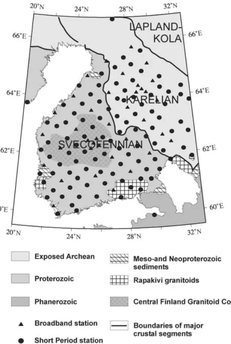
Figure 1. Simplified geological map of the study area in the Fennoscandian Shield (Boyd et al. 1985) with station array location.
lithosphere–asthenosphere boundary (LAB) and any possible tran-sition between the different tectonic units under the SVEKALAPKO area. The SVEKALAPKO seismic array consists of 143 seismic sta-tions (88 short-period and 40 broad-band, including 15 permanent stations), along a 1000 km by 900 km array covering southern and central Finland, and part of Russian Karelia. The stations were op-erated from 1998 August to 1999 May (Raita 2001). The spacing between short-period stations was 50 km and between broad-band stations 100 km (Fig. 1).
Thermal studies indicate typical thicknesses of the lithosphere between 200 and 300 km for Archean and early Proterozoic realms (Artemieva & Mooney 2001). In general, thick (>300 km) roots are found for the Baltic Shield, Siberian Platform, West Africa and pos-sibly the Canadian Shield from thermal-based studies. The structure of the lithosphere under the Baltic Shield has been a major target for researchers over the last decades. Several geophysical methods have been used to investigate this. First attempts to determine the
litho-spheric seismic structure of the Baltic Shield were done based on dispersion of Rayleigh waves (Calcagnile & Panza 1978; Calcagnile 1982, 1991). Heterogeneous upper mantle down to a depth of 350 km was interpreted by the authors as the depth to which the bot-tom of the shield might extend. Sacks et al. (1979) used converted S phases at the base of the lithosphere and estimated a thickness of 250 km. Husebye & Hovland (1982) and Husebye et al. (1986) analysed the lithosphere–asthenosphere boundary in southern Swe-den by inverting P-wave traveltime residuals. The results from this work indicated pronounced seismic anomalies down to 300 km. Bannister et al. (1991) estimated the sub-Moho velocities using a tomographic conjugate gradient inversion. Perchuc & Thybo (1996) proposed a seismic model for the Baltic Shield with a low-velocity layer between 100 and 160 km depth from long-range seismic pro-files. Bondar & Ryaboy (1997) presented a 1-D average velocity model representative for the Baltic Shield down to 800 km from deep seismic sounding observations.
In Fennoscandia the thickness of the lower crust accounts for most of the crustal thickness variation (Korja et al. 1993). The top of the lower crust under the central part of the Fennoscandian Shield is de-fined as the depth at which the P-wave velocity reaches 7.0 km s−1. The lower crust has its maximum thickness of 25 km in the same area where maximum crustal thicknesses have been modelled. The lower crust under the Baltic Shield has extraordinary geophysical charac-teristics similar to those that can be found in mantle rocks. Some authors, e.g. Korja et al. (1993), suggest that this layer consists of a combination of mafic lower crust from the island arc crustal blocks and additions from a possible delamination of the post-collisional lithosphere. In these regions of thicker crust, velocities of P waves up to 7.85 km s−1are observed just above the Moho interface. Sandoval et al. (2003) constructed a crustal model from Controlled Source Seismology data that contained these crustal features and assessed its contributions to teleseismic wave front distortion. This approach has the advantage that is independent of the subsequent inversion and uses the available a priori knowledge of the crustal structure to calculate crustal traveltime effects on teleseismic wave fronts.
2 D AT A S E T
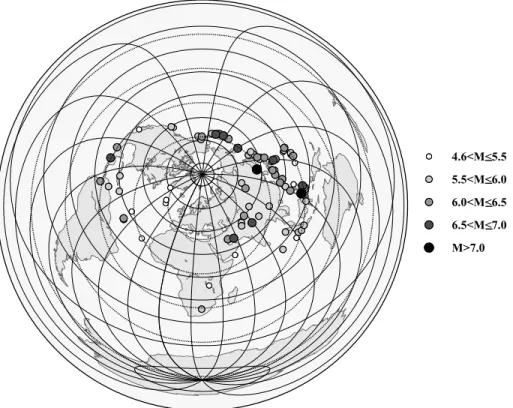
Signals from 332 selected teleseismic events were extracted from the SVEKALAPKO database. Eighty-eight high-quality events were selected for the teleseismic tomography study, and the arrival times of suitable phases after applying a proper filter were picked visually by a waveform comparison procedure. Fig. 2 shows the event distri-bution. All seismograms were restituted to simulate a short-period WWSSN (World Wide Standardized Seismographic Network) sen-sor with a dominant frequency of 1 Hz (Oliver & Murphy 1971).
For each selected earthquake, the earliest readable wavelet of P phase was first picked on a record of high signal-to-noise ratio (ref-erence station). This waveform was copied and overlaid on the other
4.6<M<5.5 5.5<M<6.0 6.0<M<6.5 6.5<M<7.0 M>7.0
Figure 2. Map showing the 88 teleseismic earthquakes used for the velocity inversion. Dotted circles denote 30◦distance marks from the centre of the SVEKALAPKO array.
records for visual correlation. This is to avoid cycle skipping (Evans & Achauer 1993) and to reduce problems associated with variations in the P waveform as it traverses the array. Theoretical traveltimes were calculated for each event and station according to the IASP91 traveltime model (Kennett & Engdahl 1991) and ellipticity correc-tions were applied. The relative traveltime residuals for each event were finally calculated by subtracting the associated mean for each event from the traveltime residuals. Because all rays to the array traverse the lower mantle essentially along the same path for each event the source and propagation path due to lower mantle effects are discarded from the data by removing the mean of the traveltime for each recorded event (Dueker et al. 1993; Evans & Achauer 1993). This is based on the hypothesis that originally underlies the ACH method (Aki et al. 1977), namely that the time residuals generated outside the given target volume are approximately constant across the seismic array. There is, therefore, a risk of leakage of deeper mantle velocity perturbations into our model (Masson & Trampert 1997).
3 M E T H O D O L O G Y
Heterogeneities along the ray path will cause seismic waves to be advanced or delayed with respect to a 1-D standard reference model at receiver locations. Teleseismic tomography involves backproject-ing the arrival-time perturbations to estimate the size and magnitude of the velocity deviations within the heterogeneous volume.
Inasmuch as the data are a relative measure of arrival times, we es-timate relative perturbations to an initial velocity model. In our case the inverse of the matrix kernel is calculated by singular value de-composition. Following Koch (1985) or Thomson & Gubbins (1982) the equivalent, non-linear system is solved iteratively.
Iterations stop when the model ceases to change significantly, which is usually achieved after a few iterations. In our case after
0 1 2 3 4 5 6 x10⁻³ 0 0.02 0.04 0.06 0.08 0.1 0.12 0.14 0.16 0.18 0.2
Cumulative model variance (km s )2 −2
Dat a variance (s ) 2 1st 2nd 3rd
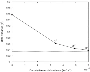
Figure 3. Variance reduction after different iterations during the
SVEKALAPKO data set inversion. The dashed line indicates the noise level which is obtained by summing the phase pick data variance and a conserva-tive error estimate in the crustal model (see text).
three iterations the optimum solution is reached with most changes to the starting model occurring in the first iteration, and only minor changes on further iterations (Fig. 3). The iterative process should be stopped early enough, to avoid fitting noise. The noise level is determined by calculating the phase pick data variance (0.0096 s2).
We added to this value a conservative estimate (20 per cent) of the traveltime error variance introduced by the crustal model (0.0256 s2)
that will be used to correct the observed traveltime residuals (San-doval et al. 2003).
Inversion based on relative traveltime residuals does not produce absolute velocity, hence the resulting velocity structure only reflects deviations about some unknown average earth model. Although the forward calculation of the theoretical traveltimes is based on a known background model, the velocity perturbations cannot be considered relative to this background model, due to the nature of the relative traveltime residuals. If the target volume is large enough, the layer-average velocities can be considered close to some commonly ac-cepted 1-D background/reference model (Leveque & Masson 1999) which should be close to the correct regional structure. Moreover, we have included in our study absolute traveltimes to constrain the layerwise average P velocity at depth. In this study, the IASP91 traveltime model (Kennett & Engdahl 1991) was used as the initial reference model for the inversion.
4 M O D E L PA R A M E T R I Z AT I O N
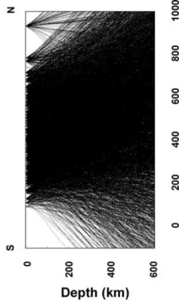
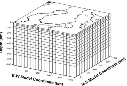
The 3-D model was parametrized by subdividing the model space into cells with velocity values constant in each cell. The spacing between the cell centres, i.e. nodes, was selected after careful ex-amination of the ray coverage (Fig. 4). This figure shows the dense (and largely homogeneous) distribution of rays throughout the inner part of the study volume. Most of the rays cross between a depth of 70 and 350 km. Therefore the resolution is expected to be highest in this depth range. The selected model parametrization has a constant grid spacing in the horizontal direction of 50 km and the grid spac-ing increases from 20 km at shallow depths to 50 km below 100 km (Fig. 5). Additional layers at 810 km depth and at±1500 km in the x- and y-directions (not shown in Fig. 5) were introduced for
stabil-ity of the inversion. The results discussed in the following sections refer to the central part of the model space only. The grid size chosen provides a high and uniform resolution to delineate upper mantle velocity variations beneath the SVEKALAPKO array. The initial velocities of the nodes are taken from the IASP91 model (Ken-nett & Engdahl 1991). Velocity was linearly interpolated between nodes for traveltime computations (Steck & Prothero 1991). The sta-tion spacing (50 km, Fig. 1) is relatively large in relasta-tion to crustal structures, as is the lateral grid spacing in the inversion (50× 50 km). Therefore teleseismic tomography cannot resolve near-surface structure (Sandoval et al. 2003) and we choose to a priori correct for 3-D crustal structure rather than including the shallow structure in the inversion.
An initial ray tracing through the 1-D reference model was per-formed to determine which nodes would be inverted. Nodes were left floating during the inversion if they were sampled by at least one ray. This yielded a total number of 4481 model parameters for the crustal corrected inversions and 4850 for the non-crustal corrected inversions. The number of rays used in the inversion was 5765.
5 R E S O L U T I O N A S S E S S M E N T
The reliability of any tomographic image depends on two factors: the spatial resolution of the image, and the standard error of the model parameters. A meaningful and reliable interpretation of to-mographic results requires the use of different methods to assess resolution capabilities, e.g. hit matrix, derivative weighted sum, ray density tensor, resolution matrix and synthetic tests (Kissling 1988) including checkerboard sensitivity tests. Synthetic tests, in partic-ular, can provide useful information about model parametrization, resolution capability of the actual data set and damping. Checker-board or ‘spike’ tests are most commonly used (Zhao et al. 1992; Benz et al. 1996; Bijwaard et al. 1998; Zelt 1998) and provide im-portant information to assess image blurring.
5.1 Hit matrix
The hit matrix is the most basic and crude approximation for assess-ing the resolution in any teleseismic study by the calculation of the number of rays that traverse a specific cell.
The hit matrix for the SVEKALAPKO data set is shown in Fig. 6. The upper layers corresponding to the crust (0, 20, 40 and 70 km depth) have a large number of hits due to the convergence of the ray paths beneath the seismic stations. The apparent very high resolution of the crust is misleading, since all rays traversing these cells are subvertical and there is no cross coverage. There is a higher density of hits beneath the centre of the array and a drift of this higher hit density area to the northeast for the deeper layers. This is due to the predominance of events incoming from these azimuths.
From the results of Fig. 6 It is difficult to clearly assess the differ-ence of resolution at intermediate and deep layers and the hit matrix appears to be an insufficient and potentially misleading element for the assessment of resolution. In this study, the hit matrix was used only as a base criterion to decide which nodes were left floating in the inversion. Cells with at least one hit were selected for inversion.
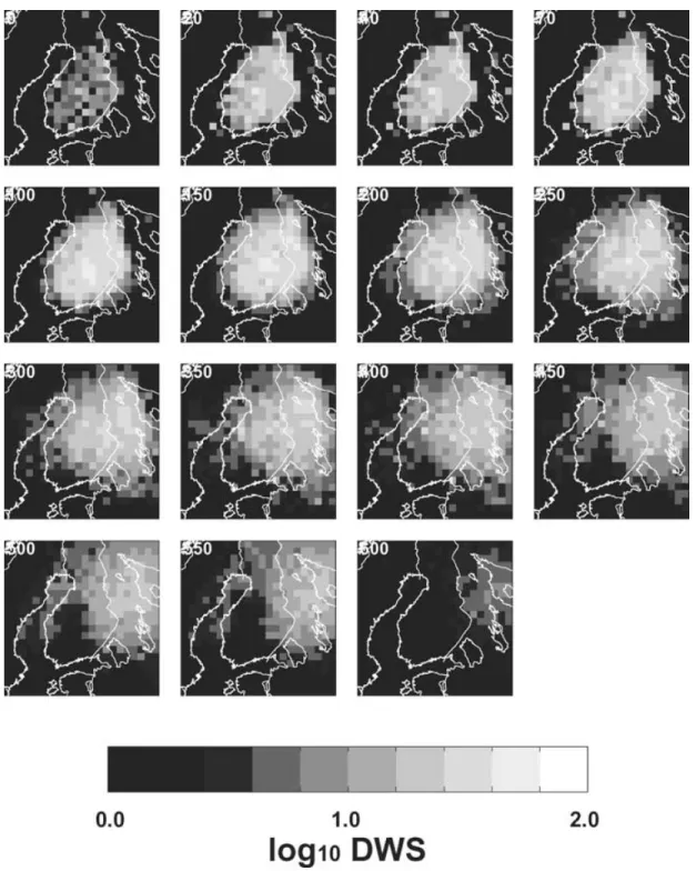
5.2 Derivative weighted sum (DWS)
The DWS (Thurber 1983; Eberhart-Phillips 1986) also takes into ac-count the number of rays that sample each cell. The DWS considers the normalized length of each ray within the cell and an observa-tional weight for that specific ray.
Figure 4. Ray coverage provided by the 5765 rays used in the inversion.
For the SVEKALAPKO data set, the DWS (Fig. 7) values reach a maximum between 100 and 350 km depth. For the quality of a tomographic image regions of homogeneously high resolution are more important than individual cells of exceptional high-resolution values (Haslinger & Kissling 2001). Notice the rather smooth vari-ation of the DWS in the well resolved layers. Comparison of Figs 6 and 7 clearly demonstrates the improvement of the resolution as-sessment of DWS over the hit count matrix. Whereas the hit matrix overestimates resolution in the shallow and bottom layers, the DWS provides a more realistic evaluation. The most important limitation of DWS is its disregard of the ray directions. This information is exploited by the calculation of the ray density tensor.
5.3 Ray density tensor (RDT)
The RDT was first defined by Kissling (1988) to assess the ray dis-tribution within an inversion block. It consists in the construction of a spatial tensor that defines the directional density of rays that cross
each cell. By analysing the ratio of its three eigenvalues representing the x, y, and z directions one gets a qualitative measure of the ray distribution at each cell.
The eigenvalues and associated eigenvectors define an ellipsoid. If, for example, rays are distributed equally in all directions within the inversion cell all three eigenvalues are nearly equal (the ellipsoid becomes a sphere). The information extracted from the eigenvalues is their standard deviation (shape of the ellipsoid) and their mean value (size of the ellipsoid). This last parameter is basically the DWS.
Although the RDT has been developed for linear inverse methods, it represents a satisfying indicator of the spatial resolution in non-linear tomography (Zollo et al. 2000).
The advantages of the RDT are:
(1) Can be easily displayed together with the solution and thus allows judgment of the credibility of a result. It can be calculated prior to the inversion.
Depth (km)
E-W Model Coordinate
(km) N-SModel Coordinate
(km)
Figure 5. Block diagram showing model parametrization. The 50 km horizontal spacing is constant all over the model space, but the vertical spacing varies
from 20 km in the topmost layer to 50 km at 600 km depth.
(2) It permits a good control on the model parametrization. (3) It is very fast to calculate.
In general all the above resolution methods resulted in similar resolution estimates. The resolution is maximum beneath the array between 70 and 350 km. This is the depth interval in which the inversion images are expected to yield the most accurate velocity estimates.
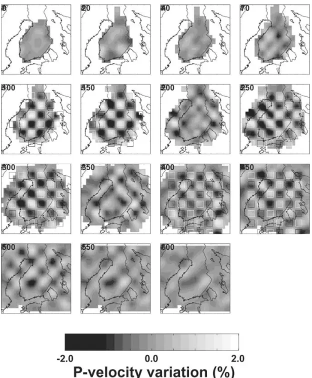
5.4 Sensitivity test
The last resolution test we performed prior to the inversion of the real data set was a sensitivity test. The main difference between sensitivity tests and synthetic tests is that in the former the same anomaly is placed throughout all the model space (Spakman et al. 1993). This allows a direct comparison of the recovered anomalies in the different regions of the model space. Usually, sensitivity tests are carried out before synthetic tests and the real data inversion,. The aim of sensitivity tests is qualitative assessment of resolution throughout the region of study, whilst synthetic tests are designed to quantitatively assess resolution in specific situations and regions, for example by mimicking recovered anomalies (Haslinger et al. 1999). In our case, we constructed a mantle structure comprising alternating positive and negative anomalies (white and black out-lines in Fig. 8) with an extension of 100× 100 × 100 km separated 50 km from each other. To analyse the amount of vertical leakage typical of this kind of experiment we left some depth levels without any anomaly (crust, 200 km, 350 km, 500 km, 550 km and 600 km depth levels). Traveltime residuals were computed using the same source and receiver locations as those of the SVEKALAPKO ex-periment (Figs 1 and 2). Gaussian-distributed noise (σ = 0.1 s) was added to the synthetic data set before it was inverted using the same parameters as for the real inversion.
The recovered anomalies (Fig. 8) are in good agreement with the input anomalies (white and black outlines) between depths of 100 and 450 km. A small amount of horizontal leakage exists but, as expected, it is smaller than the vertical leakage present at depths of 200 and 350 km. At 500 km depth, a strong downward leak-age is observed to 600 km depth. At these depths the ray crossing
is practically non-existent and the resolution is thus low (Figs 6 and 7).
6 3 - D U P P E R M A N T L E S T RU C T U R E
In the current work, the 3-D crustal model constructed by Sandoval et al. (2003) was used a priori in the inversion to correct the trav-eltime effect of the crust (upper 70 km of the model) with respect to the 1-D IASP91 model (Kennett & Engdahl 1991). The results are shown before and after the crustal correction for comparison. In the crustal-corrected inversion the first three layers (representing the crust) were fixed during the inversion.
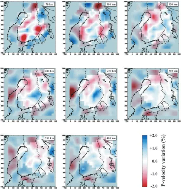
The inversion results (Figs 9, 10 and 11) show the velocity per-turbations as variations relative to the IASP91 model. However, the true layer-average velocities remain unknown because we have used relative arrival-time residuals. The transition between areas of rela-tively low and relarela-tively high velocity is depicted as white strips.
The teleseismic inversion without crustal corrections (Fig. 9) shows overall P-velocity anomalies ranging between±2 per cent. The most remarkable feature is a positive anomaly in the centre of the study area between 70 km and 250 km depth. At 300 km it is still visible but with smaller amplitude, probably due to the verti-cal leakage. Strong negative anomalies around this positive nucleus at shallow levels (70 and 100 km depth) are likely to be produced by the thick crust and are probably projected downward. At these shallow levels a positive anomaly near the southern coast of Finland coincides with the Rapakivi granitoids (Fig. 1). This result shows no evidence of the tectonic suture between the Archean and Proterozoic terranes (Fig. 1).
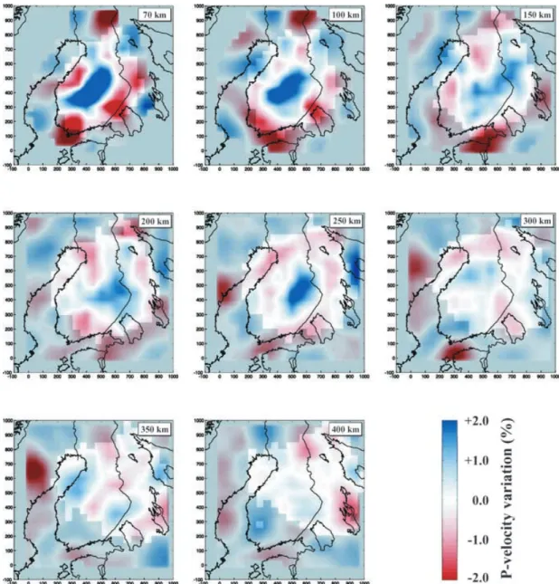
The inversion results after correction for crustal contribution (Fig. 10) show a significant increase of clarity in the recovered anomalies, in particular regarding the size and amplitude of the pos-itive nucleus. However, the depth extent of this anomaly is the same in both inversions. The shallowest level of 70 km is expected to show the largest differences between both inversions due to its proximity to the crust. The positive anomaly related to the granitic intrusion in southern Finland has largely disappeared after the crustal correc-tions supporting the crustal origin of this anomaly. The results also show no feature that could be related with the Archean–Proterozoic suture.
Figure 6. Horizontal sections at different depths (upper left corner, in km) of the hit matrix for the SVEKALAPKO experiment. For scaling see Fig. 5.
The results in Fig. 11 show P-velocity variations of up to 4 per cent in the uppermost 200 km. The positive anomaly extending down to a depth of 300 km (white arrow) is located beneath the intersection point between the profile and the tectonic suture between the Kare-lian and Svecofennian terrains (Fig. 11a) extending 300 km in an approximate E–W direction A remarkable feature in this inversion result without crustal correction is the shallow negative anomalies (−2 per cent) extending down to 200 km depth (yellow arrows, Figs 11b, e). These strong anomalies are highly influenced by the crust, and particularly by the Moho topography. The result after ap-plying crustal correction shows a significant reduction of the shallow negative anomalies. Therefore, these anomalies must be associated with crustal structure. The base of the positive anomaly is stronger
and remains unaltered (white arrow) close to 300 km depth. This positive anomaly is especially strong at 250 km depth.
7 D I S C U S S I O N
The structure and evolution of the Baltic Shield lithosphere has been studied in detail using several geophysical methods. Guggisberg et al. (1991) tentatively proposed a depth of about 180– 200 km for the LAB based on P-wave recordings of the long-range refraction seismic project FENNOLORA. Their model shows a re-duction of 1.7 per cent in P-wave velocity in a thin low velocity layer (LVL) below this boundary (about 50 km thickness beneath central
Figure 7. Horizontal sections at different depths (upper left corner, in km) of the derivative weighted sum for the SVEKALAPKO experiment. For scaling see
Fig. 5.
Sweden). According to the TOR results (Arlitt 1999; Shomali & Roberts 2002) the existence and depth of this upper boundary of a layer with reduced P-wave velocity is very questionable. No reduced P velocity was found in that study down to 300 km depth beneath this southwestern part the shield region. It is possible that veloc-ity perturbations are smeared over this boundary and, therefore, the boundary is not resolved by our data. Large low-velocity zones in S-wave velocities are more reliably identified by an analysis of sur-face wave dispersion. Calcagnile (1991) derived a model with the top of a LVL at 210 km depth beneath the central Baltic Shield from dispersion of surface waves. Perchuc & Thybo (1996) and Thybo &
Perchuc (1997) show a different result. These authors proposed the existence of a 40 km thick, 100 km deep LVL beneath a stratified mantle from the study of strong, scattered reflections beyond 8◦. This LVL is also found by Abramovitz et al. (2002) after inverting traveltime data (P and S) from the long-range deep seismic sounding experiment FENNOLORA. These features are interpreted by these authors as the presence of small amounts of partial melts or possibly free fluids, in the 100–150-km depth interval.
Toward the centre of the shield, the recovered anomaly contrasts in SVEKALAPKO are smaller in amplitude than those at the south-ern edge of the shield. The base of the positive anomaly at 300 km
Figure 8. Horizontal sections at different depths (upper left corner, in km) of the sensitivity test performed for the SVEKALAPKO experiment (see text).
White and black outlines correspond to the location of the input anomalies (+2 per cent and −2 per cent velocity variation, respectively). Grey shading gives the recovered output anomalies. For scaling see Fig. 5.
depth could represent the LAB. In this way, the lithosphere thick-ness would increase from southern Sweden (75 km) to the central part of the Fennoscandian Shield (∼300 km). However, preliminary results from dispersion of Rayleigh waves from SVEKALAPKO data show no evidence of a clear seismic asthenosphere beneath the Fennoscandian Shield (Bruneton et al. 2002; Funke & Friederich 2002).
In the TOR experiment, and following the same methodology as in this work, Arlitt (1999) derived an upper mantle model than spanned across the Tornquist Zone and extended to the southern rim of the Baltic Shield. The results suggest the existence of very thick
(>200 km) continental lithosphere of the Baltic Shield with no indi-cation of an asthenosphere. However, despite the similarities of the method used to derive the SVEKALAPKO and TOR results there are many factors that do not permit a direct correlation between the obtained mantle models. The methodology applied in both cases permits a rather precise determination of relative lateral velocity variations in the upper mantle relative to unknown background ve-locity models, and they cannot be converted directly into absolute seismic velocities for comparison with other regions. Moreover, differences in resolution, parametrization and damping make this correlation even more complex.
Figure 9. Horizontal sections at different depths (upper right corner, in km) of the recovered upper mantle structure after inverting the observed traveltime
residuals without crustal corrections. The crustal layers are left floating during the inversion (not shown). To (partially) overcome these difficulties a comparison between
traveltimes from a common event recorded at both arrays would help. In this way differences between the residuals at each array would constrain the regional variation of velocities. Unfortunately, the SVEKALAPKO and TOR experiments were carried out with a difference of 1 yr, and for this reason databases do not overlap. Nev-ertheless, we selected six additional events (Table 1) with different azimuths from the TOR database and compared the residuals with those from five stations of the Finnish permanent network (also part of the SVEKALAPKO array, Fig. 1).
Fig. 12 shows the traveltime residuals for TOR and SVEKALAPKO (after removing the average traveltime) for the six selected events. The relative residuals range between±2.0 s and the relative residual pattern is fairly independent of the incoming azimuth. The stations located on the Svecofennian Shield have trav-eltimes that, in general, are 1 to 3 s smaller than those belonging to stations in northern Germany and Denmark. Within the Sve-cofennian Shield, the lateral variations are smaller than at the tran-sition observed across the Tornquist Zone. The stations in southern
Sweden belonging to the TOR experiment have similar residuals as those from the Finnish permanent network. This observation sug-gests that the bulk velocity distribution within the Svecofennian Shield is very similar. However, there are some cases (events 5 and 6) in which some Finnish stations report slightly larger residuals (less than half a second) than the Swedish ones.
Teleseismic traveltime residuals have been studied in Finland since the 1970s and station corrections have been applied accord-ingly for event location ever since. The first documentation and publication was by Noponen (1974), with most recent studies by Tarvainen et al. (1999) and Tiira (1999). Noponen (1974) reported changes of slowness with azimuth observed at arrays in Norway, Sweden and Finland. According to these observations, the smallest azimuthal changes of slowness were reported at the Finnish stations. The exact structural transition between Sweden and Finland remains unknown from this study.
Results from P-wave traveltime inversions in the Kapvaal and Zimbabwe cratons (James et al. 2001) indicate relative velocity in-creases of up to 1 per cent down to 300 km depth. However, these
Figure 10. Horizontal sections at different depths (upper right corner, in km) of the recovered upper mantle structure after inverting the observed traveltime
residuals with crustal corrections. The crustal layers (not shown) are left fixed during the inversion. authors also found smaller regions of lower velocities (−1 per cent)
and associated them with chemical modifications of the mantle dur-ing magmatic emplacement. Bokelmann & Silver (2000) inverted P and S traveltime residuals in the Canadian Shield after apply-ing crustal corrections. The authors suggest that anisotropy (due to olivine crystal preferred orientation) in the subcontinental litho-sphere causes a stronger reduction of P-wave velocity than S-wave velocity.
Bank et al. (2000) derived a mantle model from inversion of P-wave traveltime residuals for the Slave Craton in northwest Canada. According to these authors, the Slave Craton is underlain by material with high velocities (+0.5 per cent) down to 300 km depth, though some local positive traveltime anomalies can also be recognized. This depth range is very similar to the one studied in this work, but shows smaller velocity variations. In any case, these differences in velocity variation should only be taken as indicative of a tendency and compared with great care due to the aforementioned differences during the inversion schemes.
We can establish a correlation between large crustal features, xenolith-derived upper mantle chemistry and lateral variations of P-wave velocity in the uppermost mantle. The main positive velocity anomaly in the tomographic images of the upper mantle coincides spatially with the anomalous high-velocity lower crust (Korja et al. 1993) and the Central Finland Granitoid Complex (Boyd et al. 1985). It is very unlikely that the geometry and position of the relatively high-velocity keel by pure chance coincides with the position and extent of the high-velocity lower crust and of the granitic intrusions formed during the accretion of the Svecofennian block to Karelia. The surrounding Rapakivi granitoids (Fig. 1) mark a distinctively later and different event in the evolution of the Baltic Shield. The ring-shaped Rapakivi intrusions surrounding the Central Finland Granitoid Complex (Fig. 1) might have been the result of the already existing keel deflecting ascending mantle material.
The seismic observations of SVEKALAPKO (Plomerova et al. 2002) indicate anisotropy in the sublithospheric mantle. This fact may be associated with the relatively high viscosity of the keel and
Figure 11. (a, d) Geographical location of cross sections in 11b, 11c and 11e, 11f, respectively. The tectonic suture between the Archean and Proterozoic is
also depicted; (b, e) P-velocity model recovered after inverting the observed traveltime delays prior to the crustal correction. Crustal nodes are left floating during the inversion. PR-AR stands for the location of the tectonic suture along the profiles; (c, f) P-velocity model recovered after inverting the observed traveltime delays corrected for the crustal effects. Crustal nodes are fixed during the inversion. PR-AR stands for the location of the tectonic suture along the profile. The black solid line denotes the Moho depth along the profiles. The fading denotes less resolved areas. Yellow arrows mark those anomalies with crustal origin and white arrows mark the lower limit of the cratonic root (see text).
Table 1. Events used to compute relative P residuals between TOR and SVEKALAPKO. Locations and origin times are from the EHB relocated catalogue
(Engdahl et al. 1998).
Event Year Month Day Hour Minute Second Latitude Longitude Depth (km) Magnitude
1 1996 10 24 19 31 55.77 66.981 −173.164 19.8 6.1 2 1997 03 26 02 08 58.20 51.274 179.526 29.3 6.7 3 1996 10 02 11 24 52.56 45.230 151.114 52.4 6.1 4 1996 10 18 10 50 25.25 30.613 131.049 25.3 6.6 5 1996 12 10 08 36 19.46 0.893 −29.958 9.2 7.0 6 1996 11 04 17 24 58.57 7.366 −77.369 7.1 6.3
a tendency to acquire and preserve strains in its mineralogical com-ponents. Furthermore, assuming that the keel formation occurred in the early stages of the evolution of the craton and taking into account the drift of Baltica experienced ever since (Elming et al. 1993), a mechanical detachment zone would exist below 300 km. Small-scale convection (solid state creep) transports heat to the base of the lithosphere (Kukkonen et al. 2003) and could be a reasonable explanation for this phenomenon. However, there are open ques-tions about the composition of the tectosphere that lead to signifi-cant lateral variations in seismic velocity and to global and regional variations of VP/VSratios in cratons. Given that the deep keel is
pos-sibly due to formation of the continental crust by depletion of upper mantle by removal of partial melts, the resulting mineralogy should favour olivine, garnet and orthopyroxene, whereas clinopyroxene would be reduced. On the other side, kimberlite-derived xenoliths from the keel area provide important constraints and suggest differ-ent explanations for the formation and origin of the root. Peltonen et al. (1999) suggest a stratified lithospheric mantle adjacent to the suture between the Archean and Proterozoic terranes. The man-tle in this area would be composed of a shallow, strongly depleted garnet-spinel facies underlain by a more fertile garnet facies man-tle. This garnet facies would, according to these authors, represent
1.
2.
3.
4.
5.
6.
Figure 12. Relative P-wave traveltime residuals for stations at the TOR array and five stations from the Finnish permanent network for six selected teleseismic
events (Table 1) from different azimuthal regions. The black arrows indicate the incoming direction of the teleseismic wavefront.
the geochemical signature of either a subducted Proterozoic oceanic lithosphere subducted beneath the craton margin or a post-orogenic cumulate derived from basaltic melts. More recently, Peltonen et al. (2002) analysed xenoliths from this region at a depth interval of 150– 230 km. The chemical and isotopic composition of minerals favour the latter hypothesis of the (Proterozoic?) mantle-derived melts or cumulates rather than subducted oceanic lithosphere.
8 C O N C L U S I O N S
We have presented a 3-D upper mantle model beneath Fennoscan-dia characterized by a central positive anomaly that can be traced to a depth of 300 km (Fig. 11) beneath the contact of the Archean and Proterozoic realms. Other shallower mantle anomalies could be related to surface geological features and they were successfully removed from the mantle velocity model by crustal corrections. Neither the results from our study nor from surface wave studies (Bruneton et al. 2002; Funke & Friederich 2002) support the ex-istence of a seismic asthenosphere comparable to the reduction in seismic velocities derived in the southern part of the TOR experi-ment. The relative P arrivals at TOR and SVEKALAPKO stations show arrivals between 2 and 3 s earlier for stations situated on the Svecofennian Shield than those in the North German basin. Such variations in traveltime are not observed between stations within the Svecofennian Shield of Sweden and Finland, suggesting a similar velocity structure. The addition of a significant number of absolute
P traveltimes to define the layerwise average P velocity at depth and the comparison of absolute traveltimes including TOR data al-lowed us to estimate the difference in absolute velocity over the depth range of 300 km between the shield and across the trans-European suture zone (TESZ) into mid-age continental trans-European lithosphere. As the aforementioned evidence documents, there is no low-velocity layer beneath the Baltic Shield within the top 300 km of even remotely similar features like the pronounced asthenosphere in the depth range 120 to 300 km beneath Phanerozoic Europe. We correlate the structural features at depth obtained from the tomo-graphic inversion with anomalous crustal elements and geological attributes. All these elements can help to reveal the complex evo-lution of Baltica and provide a direct link between the geological processes observed at the surface and the geodynamic activity of the upper mantle beneath cratons.
A C K N O W L E D G M E N T S
The following institutions participate in the SVEKALAPKO project: the Universities of Oulu, Helsinki, Uppsala, Grenoble, Strasbourg, Stuttgart, St Petersburg, the Kola Science Center, the Institute of Physics of the Earth Moscow, ETH Zurich, GFZ Potsdam, the Geophysical Institute of CAS Prague, and Spezge-ofisika MNR Moscow. The SVEKALAPKO project has been sup-ported by national science funding agencies in Finland, France, Swe-den and Switzerland, by the Institute of Geophysics of the Polish
Academy of Sciences, by GeoForschungsZentrum Potsdam (GFZ), by the GFZ Geophysical Instrument Pool and by an EU INTAS grant. Thanks are due to the European Science Foundation (ESF) for supporting several workshops of the SVEKALAPKO groups in St Petersburg and Lammi, Finland through their international programme EUROPROBE. We are very grateful to the Institute of Seismology of Helsinki, especially to L. Tellervo and A. Korja, for the data provided from their permanent network used in this paper. Finally, we would like to thank Hans Thybo and an anonymous re-viewer for their constructive reviews. Contribution number 1329, Institute of Geophysics, ETH Zurich.
The SVEKALAPKO Seismic Tomography Group is formed by: U. Achauer, A. Alinaghi, J. Ansorge, G. Bock, M. Bruneton, W. Friederich, M. Grad, P. Heikkinen, S.E. Hjelt, T. Hyvonen, J.P. Ikonen, E. Kissling, K. Komminaho, A. Korja, E. Kozlovskaya, H. Paulssen, N. Pavlenkova, H. Pedersen, J. Plomerova, T. Raita, O. Riznitchenko, R.G. Roberts, S. Sandoval, I.A. Sanina, N. Sharov, E. Wielandt, K. Wylegalla and J. Yliniemi.
R E F E R E N C E S
Abramovitz, T., Thybo, H. & Perchuc, E., 2002. Tomographic inversion of seismic P- and, S-wave velocities from the Baltic Shield based on FENNOLORA data, Tectonophysics, 358, 151–174.
Aki, K., Christoffersson, A. & Husebye, E.S., 1977. Determination of 3-dimensional seismic structure of lithosphere, J. geophys. Res., 82, 277– 296.
Arlitt, R., 1999. Teleseismic body wave tomography across the trans-European suture zone between Sweden and Denmark. PhD Thesis, ETH, Zurich, p. 126.
Artemieva, I.M. & Mooney, W.D., 2001. Thermal thickness and evolution of Precambrian lithosphere: a global study, J. geophys. Res.-Solid Earth,
106, 16 387–16 414.
BABEL, Working Group, 1993. Integrated seismic studies of the Baltic shield using data in the Gulf of Bothnia region, Geophys. J. Int., 112, 305–324.
Bank, C.G., Bostock, M.G., Ellis, R.M. & Cassidy, J.F., 2000. A reconnais-sance teleseismic study of the upper mantle and transition zone beneath the Archean Slave craton in NW Canada, Tectonophysics, 319, 151–166. Bannister, S.C., Ruud, B.O. & Husebye, E.S., 1991. Tomographic estimates of sub-Moho seismic velocities in Fennoscandia and structural implica-tions, Tectonophysics, 189, 37–53.
Benz, H.M., Chouet, B.A., Dawson, P.B., Lahr, J.C., Page, R.A. & Hole, J.A., 1996. Three-dimensional P and S wave velocity structure of Redoubt Volcano, Alaska, J. geophys. Res.-Solid Earth, 101, 8111–8128. Bijwaard, H., Spakman, W. & Engdahl, E.R., 1998. Closing the gap between
regional and global travel time tomography, J. geophys. Res.-Solid Earth,
103, 30 055–30 078.
Blundell, D.J., Freeman, R. & Mueller, S., 1992. A Continent Revealed. The
European Geotraverse. Cambridge University Press, Cambridge, p. 275.
Bokelmann, G.H.R. & Silver, P.G., 2000. Mantle variation within the Canadian Shield: travel times from the portable broadband Archean-Proterozoic transect 1989, J. geophys. Res.-Solid Earth, 105, 579–605. Bondar, I. & Ryaboy, V., 1997. Regional travel-time tables for the Baltic
Shield region, Technical Report, CMR-97/24. Center for Monitoring Re-search, Arlington, VA.
Boyd, R., Nilsson, G., Papunen, H., Vorma, A., Zagorodny, V. & Robonen, V., 1985. General geological map of the Baltic Shield, in Nickel-copper
Deposits of the Baltic Shield and Scandinavian Caledonides, p. 394, eds,
Papunen H. & Gorbunov G.I., Geol. Survey of Finland, Helsinki. Bruneton, M., Pedersen, H.A., Farra, V. & the SSTW Group, 2002.
Surface-wave tomography in Fennoscandia, Geophys. Res. Abs., Vol. 4, 02733, 27th General Assembly of the European Geophysical Society, Nice, France, 21–26 April, 2002.
Calcagnile, G. & Panza, G.F., 1978. Crust and upper mantle structure
un-der Baltic Shield and Barents Sea from dispersion of Rayleigh waves,
Tectonophysics, 47, 59–71.
Calcagnile, G., 1982. The lithosphere asthenosphere system in Fennoscan-dia, Tectonophysics, 90, 19–35.
Calcagnile, G., 1991. Deep-structure of Fennoscandia from fundamental and higher mode dispersion of Rayleigh waves, Tectonophysics, 195, 139–149. Dueker, K.G., Humphreys, E.D. & Biasi, G., 1993. Teleseismic velocity tomography using the ACH method: theory and application to continental-scale studies, in Seismic Tomography: Theory and Practice, pp. 265–298, eds Iyer, H.M. & Hirahara, K., Chapman & Hall, London.
Eberhart-Phillips, D., 1986. 3-dimensional velocity structure in Northern California Coast Ranges from inversion of local earthquake arrival times,
Bull. seismol. Soc. Am., 76, 1025–1052.
Elming, S.A. et al., 1993. The drift of the Fennoscandian and Ukrainian shields during the Precambrian—a paleomagnetic Analysis,
Tectono-physics, 223, 177–198.
Engdahl, E.R., van der Hilst, R. & Buland, R., 1998. Global teleseismic earthquake relocation with improved travel times and procedures for depth determination, Bull. seismol. Soc. Am., 88, 722–743.
Evans, B. & Achauer, U., 1993. Teleseismic velocity tomography using the ACH method: theory and application to continental-scale studies, in
Seis-mic Tomography: Theory and Practice, pp. 319–360, eds Iyer, H.M. &
Hirahara, K., Chapman & Hall, London.
Funke, S. & Friederich, W., 2002. Rayleigh wave dispersion and a 1D S-velocity model of the Fennoscandian mantle, in Geophys. Res. Abs., Vol.
4, 04285, 27th General Assembly of the European Geophysical Society,
Nice, France, 21–26 April, 2002.
Gee, D.G. & Zeyen, H., 1996. EUROPROBE 1996-Lithosphere Dynamics:
Origin and Evolution of Continents, p. 138, EUROPROBE Secretariat,
Uppsala University, Uppsala.
Gorbatschev, R. & Bogdanova, S., 1993. Frontiers in the Baltic Shield,
Pre-cambrian Res., 64, 3–21.
Guggisberg, B., Kaminski, W. & Prodehl, C., 1991. Crustal structure of the Fennoscandian Shield—a traveltime interpretation of the long-range Fennolora seismic refraction profile, Tectonophysics, 195, 105. Haslinger, F. et al., 1999. 3D crustal structure from local earthquake
tomogra-phy around the Gulf of Arta (Ionian region, NW Greece), Tectonotomogra-physics,
304, 201–218.
Haslinger, F. & Kissling, E., 2001. Investigating effects of 3-D ray tracing methods in local earthquake tomography, Phys. Earth planet. Int., 123, 103–114.
Husebye, E.S. & Hovland, J., 1982. On upper mantle seismic heterogeneities beneath Fennoscandia, Tectonophysics, 90, 1–17.
Husebye, E.S., Hovland, J., Christoffersson, A., Astrom, K., Slunga, R. & Lund, C.E., 1986. Tomographic mapping of the lithosphere and astheno-sphere beneath southern Scandinavia and adjacent areas, Tectonophysics,
128, 229–250.
James, D.E., Fouch, M.J., Van Decar, J.C. & van der Lee, S., 2001. Tecto-spheric structure beneath southern Africa, Geophys. Res. Lett., 28, 2485– 2488.
Jordan, T.H., 1978. Composition and development of continental tecto-sphere, Nature, 274, 544–548.
Kennett, B.L. N. & Engdahl, E.R., 1991. Traveltimes for global earthquake location and phase identification, Geophys. J. Int., 105, 429–465. Kissling, E., 1988. Geotomography with local earthquake data, Rev.
Geo-phys., 26, 659–698.
Koch, M., 1985. Nonlinear inversion of local seismic travel-times for the si-multaneous determination of the 3D-velocity structure and hypocentres— application to the seismic zone Vrancea, Journal of Geophys., 56, 160– 173.
Korja, A., Korja, T., Luosto, U. & Heikkinen, P., 1993. Seismic and geoelec-tric evidence for collisional and extensional events in the Fennoscandian Shield—implications for Precambrian crustal evolution, Tectonophysics,
219, 129–152.
Kukkonen, I., Kinnunen, K. & Peltonen, P., 2003. Mantle xenoliths and thick lithosphere in the Fennoscandian Shield. Geophys. Res. Abs., Vol.
5, 03520, 28th General Assembly of the European Geophysical Society,
Leveque, J.J. & Masson, F., 1999. From ACH tomographic models to absolute velocity models, Geophys. J. Int., 137, 621–629.
Masson, F. & Trampert, J., 1997. On ACH, or how reliable is regional tele-seismic delay time tomography? Phys. Earth planet. Inter., 102, 21–32. Meissner, R. & Wever, T., 1986. Intracontinental seismicity, strength of
crustal units, and the seismic signature of fault zones, Phil. Trans. R. Soc.
Lond., A, 317, 45–61.
Noponen, I., 1974. Seismic ray direction anomalies caused by deep structure in Fennoscandia, Bull. seismol. Soc. Am., 64, 1931–1941.
Oliver, J. & Murphy, L., 1971. WWSSN—seismology’s global network of observing stations, Science, 174, 254–261.
Peltonen, P., Huhma, H., Tyni, M. & Shimizu, N., 1999. Garnet peridotite xenoliths from kimberlites of Finland: nature of the continental mantle at an Archean craton–Proterozoic mobile belt transition, in VIIth
Inter-national Kimberlite conference, Vol. 2, pp. 664–676, eds, Gurney, J.J.,
Gurney, J.L., Pascoe, M.D. & Richardson, S.H., National Book Printers, Cape Town, South Africa.
Peltonen, P., Kinnunen, K.A. & Huhma, H., 2002. Petrology of two diamon-diferous eclogite xenoliths from the Lahtojoki kimberlite pipe, eastern Finland, Lithos, 63, 151–164.
Perchuc, E. & Thybo, H., 1996. A new model of upper mantle P-wave velocity below the Baltic Shield: indication of partial melt in the 95 to 160 km depth range, Tectonophysics, 253, 227–245.
Plomerova, J., Hyvonen, T., Sandoval, S., Babuska, V. & the SSTW Group, 2002. Structure of Fennoscandian mantle from seismic veloc-ity anisotropy, in Geophys. Res. Abs., Vol. 4, 02173, 27th General As-sembly of the European Geophysical Society, Nice, France, 21–26 April, 2002.
Raita, T., 2001. The seismic tomography experiment of the SVEKALAPKO project, Pro graduate Thesis, University of Oulu, Finland, p. 96. Sacks, I.S., Snoke, J.A. & Husebye, E.S., 1979. Lithosphere thickness
be-neath the Baltic Shield, Tectonophysics, 56, 101–110.
Sandoval, S., Kissling, E. & Ansorge, J., 2003. High-resolution body wave tomography beneath the SVEKALAPKO array: I. A priori three-dimensional crustal model and associated traveltime effects on teleseismic wave fronts, Geophys. J. Int., 153, 75–87.
Shomali, Z.H. & Roberts, R.G., 2002. Non-linear body wave teleseismic tomography along the TOR array, Geophys. J. Int., 148, 562–574. Spakman, W., Vanderlee, S. & Vanderhilst, R., 1993. Travel-time
tomogra-phy of the European Mediterranean mantle down to 1400 km, Phys. Earth
planet. Inter., 79, 3–74.
Steck, L.K. & Prothero, W.A., 1991. A 3-D raytracer for teleseismic body-wave arrival times, Bull. seismol. Soc. Am., 81, 1332–1339.
Tarvainen, M., Tiira, T. & Husebye, E.S., 1999. Locating regional seismic events with global optimization based on interval arithmetic, Geophys. J.
Int., 138, 879–885.
Thomson, C.J. & Gubbins, D., 1982. 3-dimensional lithospheric modeling at Norsar—linearity of the method and amplitude variations from the anomalies, Geophys. J. R. astron. Soc., 71, 1–36.
Thurber, C.H., 1983. Earthquake locations and 3-dimensional crustal struc-ture in the Coyote Lake area, central California, J. geophys. Res., 88, 8226–8236.
Thybo, H. & Perchuc, E., 1997. The seismic 8 degrees discontinuity and partial melting in continental mantle, Science, 275, 1626–1629. Tiira, T., 1999. Slowness vector correction for teleseismic events with
arti-ficial neural networks, Phys. Earth planet. Inter., 112, 101–109. Zelt, C.A., 1998. Lateral velocity resolution from three-dimensional seismic
refraction data, Geophys. J. Int., 135, 1101–1112.
Zhao, D., Horiuchi, S. & Hasegawa, A., 1992. Seismic velocity structure of the crust beneath the Japan Islands, Tectonophysics, 212, 289–301. Zollo, A., De Matteis, R., D’Auria, L. & Virieux, J., 2000. A 2D non linear
method for travel time tomography: application to Mt Vesuvius active seismic data, in, Problems in geophysics for the new millenium, pp. 125– 140, Editorice Compositori, Bologna.