Fourier optics: basic concepts

(1)

HAL Id: hal-01741583

https://hal.archives-ouvertes.fr/hal-01741583

Preprint submitted on 23 Mar 2018

HAL is a multi-disciplinary open access

archive for the deposit and dissemination of

sci-entific research documents, whether they are

pub-lished or not. The documents may come from

teaching and research institutions in France or

abroad, or from public or private research centers.

L’archive ouverte pluridisciplinaire HAL, est

destinée au dépôt et à la diffusion de documents

scientifiques de niveau recherche, publiés ou non,

émanant des établissements d’enseignement et de

recherche français ou étrangers, des laboratoires

publics ou privés.

Fourier optics: basic concepts

Stéphane Perrin

To cite this version:

(2)

Fourier optics: basic concepts

Stephane Perrin

*

ICube, UMR CNRS 7357 - University of Strasbourg, FR-67412 ILLKIRCH

February 21, 2018

Based on diffraction theory and the propagation of the light, Fourier optics is a powerful tool allowing the esti-mation of a visible-range imaging system to transfer the spatial frequency components of an object. The analyses of the imaging systems can thus be performed and the the performance retrieved. For a better understanding of the optical study, we present a short introduction of the Fourier optics and we review the mathematical treat-ment depending on the illumination conditions of the imaging system. Furthermore, resolution criteria based on Fourier optics are detailed. Also, the impact of aberrations on the imaging quality are discussed.

INTRODUCTION

The performance of a linear optical system can be evalu-ated using Fourier optics [1]. Indeed, the ability of a sin-gle lens or a more complex system to reproduce an im-age of an (1D or 2D) object can be quantify by decom-posing the object in Fourier series. In Fourier optics, the object is thus considered as a sum of spatial sinusoidal waves at specific frequencies by analogy with electron-ics [2]. Despite the resolution limit of a microscope by the diffraction of the light was explicitly mentioned by E. Verdet in 1869 [3], the concept of Fourier series de-composition appeared firstly in 1873 with the works of E. Abbe [4]. He considered the objects as periodic diffrac-tion elements and he showed that at least two orders of a diffraction grating should be collected by the objective lens of a microscope in order to barely resolve the features of the grating. He describes in words the first definition of

the spatial resolutionδx,y which can be mathematically

expressed as:

δx,y= λ n sin (θ)=

λ

N A (1)

Where λ is the wavelength of the monochromatic light

source and θ, the diffraction angle of the periodic

ob-ject. According to the Abbe theory, only diffracted com-ponents generated by the object having a spatial period

higher thanδx,yare intercepted by the finite pupil of the

lens. Thus, the features with higher spatial frequencies are not resolved. In addition, the term of numerical aper-ture (NA) were firstly introduced as the sine of the

diffrac-tion angleθ [5]. Moreover, E. Abbe reported that the

reso-lutionδx,ycan be improved using an focusing (or oblique)

illumination of the object. This assumption allows deter-mining the total NA of a microscope as the sum of the NAs of each optical component of the microscope. If the NA of

the illumination part N Aiequals the NA of the collection

part N Ac, Eq. 1 can hence be written:

δx,y= λ

N Ai+ N Ac=

λ

2 N A (2)

It should be noted that a direct focusing illumination through a Abbe condenser lens has however the disad-vantage of imaging the lamp filament on the sample. A. Köhler took an interest in illumination conditions for mi-croscopy and developed thus a method for homogenising the intensity of the incident beam using an arrangement of lenses and diaphragms [6].

In 1876, H. von Helmholtz confirmed the Abbe the-ory through a mathematical demonstration of the resolu-tion limit [7]. At the same time, he exposed the impact of the coherence of the light for avoiding the phase re-lations [8] and he showed that Eq. 1 also requires a fac-tor 1/2 when the illumination light source is incoherent (λ becomes thus λ0, the central wavelength of the

broad-band light source). Furthermore, H. von Helmholtz dis-cussed a new definition of the spatial resolution, reported previously in 1874 by Lord Rayleigh [9].

J. W. Rayleigh did not treat microscopic objects as grating elements illuminated with plane waves but rather as as a sum of white-light-emitting point sources. Us-ing the Airy works who calculated the diffraction pattern of a bright point source [10], J. W. Rayleigh defined the angular separation of an imaging system as the distance between the intensity maximum and the first intensity minimum of the diffraction pattern of an on-axis point

source1. Based on Fourier’s theorem, this definition leads

to a new resolution expression:

δx,y≈ 0.61

f λ

R (3)

Where f is the focal length of the lens and R is the ra-dius of the finite pupil of the lens. Some years later, in 1879, Lord Rayleigh presented a view equivalent to re-garding diffraction effects as resulting from the exit pupil [11]. In 1896, Lord Rayleigh extended his investigations to different objects (points, lines and gratings) and aperture shapes [12].

Twenty years later, based on the limits of photode-tectors, C. M. Sparrow defined the smallest recognizable

*_{Corresponding author: stephane.perrin@unistra.fr}

1_{The diffraction image of an emitting incoherent point source through an optical system is the point spread function (PSF) of the system.}

(3)

inter-space as the distance for which the irradiance pat-tern of two incoherent point sources has no curvature in the center [13], giving the expression:

δx,y= 0.47 λ

N A (4)

These criteria assume an aberrations-free imaging sys-tem. Nevertheless, in practice, evaluating the resolution is more complex due to the noise and the aberrations of optical components. Furthermore, the nature of the light source, i.e. coherent, partially coherent, partially inco-herent or incoinco-herent, should be considered. In 1927, W. V. Houston proposes thus to use the full-width at half-maximum (FWHM) of the diffraction pattern of a point source (being the PSF of the imaging system), to quantify the lateral resolution [14] because more useful in practice and also applicable to diffraction patterns that do not fall off to zero, i.e. a Gaussian PSF or a Lorentzian PSF.

In 1946, P.M. Duffieux introduced Fourier optics for evaluating the spatial frequency transfers through the op-tical system using sinusoidal test patterns [15]. And, lat-ter, H.H. Hopkins led the way in the use of transfer func-tion methods for the assessment of the quality of optical imaging systems, making the analogy with analog elec-tronic systems. In 1960, V. Ronchi highlighted the impor-tance of considering both the sensitivity of the sensor and the illumination conditions, to determine the resolving power of an imaging system [16].

Nowadays, Fourier optics is often used for the design of new optical components or the analysis of imaging system. And the mathematical treatment of Fourier op-tics was demonstrated and is supposed to be known [17]. However, the nature of the light dependence is often ne-glected and not considered in the literature. Thus, this manuscript reviews the influence of the coherence of the light source on the transfer function of a visible-range (or infra-red) imaging system. The resolution criteria based on Fourier optics are explained. Furthermore, the effects of aberrations on the imaging quality are discussed.

IMAGING SYSTEMS

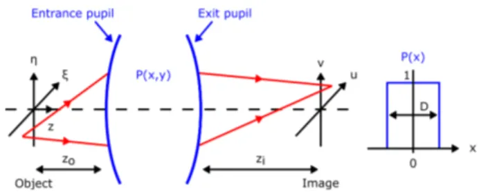
In Fourier optics, the imaging systems are supposed time invariant and linear. Figure. 1 represents a generalized scheme of an optical system, i.e. an assembly of optical elements, collecting the electric field from a point source placed in the object plane and propagating it in the image

plane. The object plane is placed at a distance zoof the

entrance pupil, i.e. the working distance, and the

imag-ing plane at a distance zi of the exit pupil. The exit pupil

(or simply the finite circular pupil function P (x, y)) of the imaging system is considered in the following diffraction equations. Indeed, only the output pupil plays a role in the diffraction of the light. The pupil function P (x, y) has a diameter D and is unity inside and zero outside the pro-jected aperture. Gauss approximations are considered, meaning that the incident angles are small and the point

light sources are close to the optical axis2.

Figure 1: Model of an imaging system and

representa-tion of its pupil funcrepresenta-tion. The electric field from the

emit-ting point source in the object plane is transmitted by the imaging system in the image plane. The imaging system has a normalized pupil function P (x, y) with a diameter

D. ξ and η are the Cartesian coordinates in the object

plane. x and y are the Cartesian coordinates in the prin-cipal planes of the imaging system. u and v are the Carte-sian coordinates in the image plane. z is the optical axis.

Furthermore, the imaging system is first assumed to be free of aberration, i.e. a diffraction-limited optical sys-tem. An imaging system is said to be diffraction-limited if a diverging spherical wave, emanating from a point-source object, is converted by the system into a new wave, again perfectly spherical, that converges towards an ideal point in the image plane, where the location of that ideal image point is related to the location of the original object point through a simple scaling factor, i.e. the magnifica-tion M . The magnificamagnifica-tion factor must be the same for all points in the lateral field of view of the imaging system [2]. In the image plane, the 2D complex amplitude distri-bution of the image of a point light source is represented by a superposition integral, Ui(u, v) = Ï ∞ ∞ h¡u, v;ξ,η¢ ×Uo ¡ ξ,η¢ dξdη, (5)

with Uo¡ξ,η¢, the complex electric field of the emitting

point source. The coordinates u and v are given by u =

Mξ and v = Mη where the magnification M of the

imag-ing system could be negative or positive. Usimag-ing the con-volution theorem [18], Eq. 5 can be rewritten:

Ui(u, v) = h¡u, v;ξ,η¢~Uo¡ξ,η¢ (6)

The amplitude response to a point-source object

h¡u, v;ξ,η¢ of the imaging system (also called amplitude

point spread function) at a position¡

ξ,η¢ is defined as the

Fourier transform of its pupil function P (x, y).

h¡u, v;ξ,η¢ = A λzi Ï ∞ ∞ P¡x, y¢× exp ½ − j_λz2π i £(u − Mξ) x + ¡v − Mη¢ y¤ ¾ dxdy (7)

In order to determine the irradiance Ii(u, v) recorded by

a photo-detector placed in the image plane, the square of the image amplitude is time-averaged.

Ii(u, v) =|Ui(u, v) |2® (8)

(4)

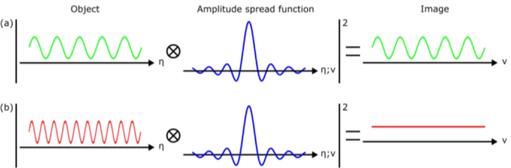
Figure 2: Spatial-domain response of an optical system in coherent imaging. The frequency of (a) the green object signal is lower than the frequency of (b) the red object signal. The image intensity is the square of the convolution product of the amplitude object with the amplitude spread function of the system.

Figure 3: Frequency-domain response of an optical system in coherent imaging. The frequency of the green object signal is lower than the frequency of the higher object signal. The image is the square of the product of the pupil function of the system with the amplitude object.

COHERENT IMAGING

The coherent illumination of an object yields an imaging system linear in complex amplitude. Indeed, by

defin-ing a time-invariant phasor amplitude Ui(u, v) in the

im-age space, the imaging system is found to be described by an amplitude convolution equation. By combining the Eq.6 and Eq.8, the expression of the image intensity can thus defined as the square of the convolution prod-uct of the object signal and the amplitude spread function

h¡u, v;ξ,η¢. Ii(u, v) = D ¯ ¯h¡u, v;ξ,η¢~U_o ¡ ξ,η¢¯¯2E (9) Figure 2 shows the image formation of an imaging system with coherent illumination in one dimensions. Assuming a rectangular-aperture amplitude distribution P (x), the

amplitude spread function h¡v;η¢, represented in blue,

is a cardinal sinus function, i.e. a zero-order spherical Bessel function. Two objects (two continuous periodical waves) having a low and a high spatial frequencies are il-lustrated in green and in red, respectively. The imaging system transmits the low frequency object pattern keep-ing the same contrast (Fig.2(a)). Whereas, when the fre-quency of the entrance signal is higher (Fig.2(b)), the con-trast of the image equals zero, i.e. the imaging system

cannot resolve such frequency. Through a frequency

analysis, a better visualization of the coherent imaging process is provided. Using convolution theorem and Eq. 6, the frequency-domain electric field in the image plane can be expressed by:

F{Ui(u, v)} =F©h ¡u, v;ξ,η¢ª ×F©Uo

¡

ξ,η¢ª, (10) and, from Eq. 7,

F{Ui(u, v)} ∝ P(x, y) ×F©Uo¡ξ,η¢ª, (11)

Then, the frequency-domain irradiance is defined by:

Ii¡ fy, fx¢ ∝

¯

¯P (x, y) ×F©U_o ¡

ξ,η¢ª¯¯2 (12) These equations show that the term of normalized

ampli-tude transfer function H¡ fx, fy¢ of the imaging system is

its pupil function P (x, y).

H¡ fx, fy¢ =F©h ¡u, v;ξ,η¢ª

∝F©F©P(x, y)ªª ∝ P ¡λzifx,λzify

¢ (13) Figure 3 illustrates the image formation in frequency do-main of a finite-aperture imaging system using a coherent illumination. The object consists of two sinusoidal sig-nals having a high and a low frequency equivalent to Fig. 2. When the frequency of the entrance object signal is

be-low the cut-off frequency fc of the imaging system, e.g.

green signal, the resulting contrast of its image stays un-changed. However, for higher frequency signal, e.g. red signal, the contrast drop to zero. The frequencies of the object being higher than the cut-off frequency of transfer function of the coherent imaging system are thus not

re-solved. The cut-off frequency fcof a perfectly-coherent

imaging system is given by:

fc= D λzi =

N A

λ (14)

This formula remind us the Abbe theory with Eq. 1. How-ever, this assumption of strictly monochromatic illumina-tion is overly restrictive. The illuminaillumina-tion generated by real optical sources, including the LASER, are never per-fectly monochromatic. The value of the cut-off frequency could hence be slightly reduced.

(5)

Figure 4: Spatial-domain response of an optical system in incoherent imaging. The frequency of (a) the green object signal is lower than the frequency of (b) the red object signal. The intensity image is the convolution product of the intensity object with the intensity spread function of the system. For an aberration-free imaging system, the intensity spread function is an Airy disk where the FWHM equals 1.029 and the first zero is at 1.219 precisely.

Figure 5: Frequency-domain response of an optical system in incoherent imaging. The frequency of the green object signal is lower than the frequency of the higher object signal. The intensity image is the product of the modulation transfer function of the system with the square of amplitude object.

INCOHERENT IMAGING

Using an incoherent illumination, the image formation by the optical system is linear in intensity. The resulting in-tensity in the image plane is defined as the square of the

amplitude spread function h¡u, v;ξ,η¢ convoluted at the

object irradiance point source. Equation 9 can thus be ex-pressed: Ii(u, v) = ¯ ¯h¡u, v;ξ,η¢¯¯ 2 ~¯ ¯U_o ¡ ξ,η¢¯¯2 (15) or, Ii(u, v) = ¯ ¯h¡u, v;ξ,η¢¯¯ 2 ~Io ¡ ξ,η¢ (16) The imaging process of an aberration-free optical system using an incoherent light source is schemed in Fig.4 in one dimension. The object having two distinct frequen-cies, as shown in Fig.2, are illustrated in green and in red. Here, the imaging system transmits the low-frequency object signal keeping the same contrast (Fig.4(a)). How-ever, when the frequency of the entrance signal is higher (Fig.4(b)), the contrast of the image is decreased but still resolved by the imaging system. The incoherent spread function, also called intensity spread function or intensity point spread function (IPSF), is the square of the

ampli-tude spread function h¡u, v;ξ,η¢ of the imaging system.

This function is called Airy disk [10] where the full width at half maximum (FWHM) equals 1.029 and the first zero

position is atη = 1.219. J. W. Rayleigh reported the use of

the first zero of the Airy pattern in order to determine the

distanceδxbetween two resolved point sources [9].

η = 1.219 = δx

2 N A

λ (17)

In frequency domain, Eq. 16 can be retrieved using the convolution theorem. F{Ii(u, v)} =F n ¯ ¯h¡u, v;ξ,η¢¯¯ 2o ×F©Io¡ξ,η¢ª, (18) or F{Ii(u, v)} ∝F n_¯ ¯F©P(x, y)ª ¯ ¯ 2o ×F©Io¡ξ,η¢ª (19)

In this equations, the term of optical transfer function

OT F¡ fx, fy¢ is revealed, being the normalized

autocorre-lation function of the amplitude transfer function.

OT F¡ fx, fy¢ =F n_¯ ¯h¡u, v;ξ,η¢¯¯ 2o ∝Fn¯¯F©P(x, y)ª ¯ ¯ 2o (20) From the Fourier transform operation, a real and an imag-inary parts result, leading to the modulation transfer function (MTF) and the phase transfer function (PTF).

M T F =¯

¯OT F

¯

¯ (21)

P T F = ang l e {OT F } (22) The PTF is liable for the transversal shift of the image. Whereas, the MTF represents the contrast (or the

visibil-ity) distribution ratio between the image Mi mag ewith the

object Mob j ec tat a given spatial frequency fx, fy.

M T F¡ fx, fy¢ =

Mi mag e Mob j ec t

¡ fx, fy¢ (23)

Where the contrast M¡ fx, fy¢ is related to the intensity

modulation depth of the sinusoid signal.

M¡ fx, fy¢ =

Imax− Imax Imax+ Imax

(6)

Figure 5 illustrates the transfer function of an incoherent imaging system with a rectangular pupil function P (x, y). The object signals are sinusoidal functions with differ-ent frequencies (see Fig. 4). An differ-entrance signal with a

frequency below the cut-off frequency fc of the transfer

function of the imaging system can be transmitted with-out reducing of the contrast. However, unlike in coher-ent imaging, the contrast of higher frequency signal than

fccan be decreased, e.g. the red higher frequency signal,

and still resolved. The cut-off frequency fcof the transfer

function in incoherent imaging is defined by:

fc= 2 N A

λ0

, (25)

confirming the results reported previously by H. von Helmholtz [7]. The long wavelengths tend thus to de-crease the cut-off frequency value. While, shorter

wave-lengths increase fc. For polychromatic illumination, the

MTF is determined by averaging the sum of M T F¡ fx, fy

¢ of each wavelength, i.e. additioning the MTFs over the bandwidth of the light source [19]. In experiments, the re-sulting polychromatic transfer function is assumed

simi-lar to the one at the central wavelengthλ0of the

spec-trum.

Mathematically, the MTF function of an aberration-free imaging system, having a circular pupil, can be ex-pressed as: M T F¡ fx, fy¢ = 2 π © φ¡fx, fy¢ − cos£φ¡fx, fy¢¤ sin£φ¡fx, fy ¢¤ª (26) where, in one dimension,

cos£ φ¡fx¢¤ = fx fc and cos£ φ¡fy¢¤ = fy fc (27)

INFLUENCE OF THE ABERRATIONS

Up to now, the manuscript relates the performance Fourier analysis of an aberration-free imaging system, i.e. a diffraction-limited system. In reality, the imag-ing systems provide often optical aberrations especially high-numerical-aperture systems. These aberrations de-crease dramatically the performance of imaging systems through the deformation of the transfer function in both spatial and frequency domain. Indeed, in spacial domain, the point spread function can be widen, lowing the lateral resolution, or can be flattened, reducing the contrast of the image. Therefore, criteria exist for estimating the per-formance of an aberrated imaging system.

The Strehl ratio (SR) allows a quantification of the contrast as a function of a perfect optical component, having the same numerical aperture [20, 21], through a mathematical operation based on the ratio of intensity peaks.

SR =max (I P SFaber r at ed)

max¡I PSFper f ec t

¢ (28)

where max (I P SFaber r at ed) is the IPSF peak intensity of

the system to be characterized and max¡I PSFper f ec t¢ is

the IPSF peak intensity of an aberration-free system. An system system is assumed diffraction limited only when

the SR is higher than 0.8. Other criteria subsist and are listed in Tab. 1.

Table 1: Relation between SR and RMS of the wavefront.

Strehl ratio RMS (wave) Criterion

0.96 λ/32

0.82 λ/14 Maréchal

0.8 λ/13.4 Diffraction limit

According to Maréchal’s Strehl approximation, the root mean square (RMS) of the wavefront can then be de-ducted from SR when the aberrations are low (SR > 0.8).

SR = exp£−(RMSPhi)2¤ (29)

In frequency domain, optical aberrations decrease the

contrast of the MTF at some frequencies fx,y or yield

to a linear lateral shift of the image pattern, i.e. PTF derivation. Figure 6 illustrates the impact of the com-monly optical aberrations on the MTF distribution. The cut-off frequency, depending on the wavelength of the light source and the NA of the imaging system, stays un-changed. However, the MTF of strongly-aberrated imag-ing system could fall off to zero at lower frequencies, lead-ing perhaps, in practice, to wrong interpretation of the re-sults.

Figure 6: Modulation transfer function of an incoherent

imaging system being aberration-free or having defocus,

spherical or astigmatism aberration.

H. H. Hopkins defined thus a criterion based on a drop-off contrast of the MTF equaling 20%, by analogy to the Strehl ratio for IPSF [19, 22].

DISCUSSIONS

First, periodic white and black bars, i.e. Ronchi rulings or USAF 1951 target, are widely preferred in experiments for example for the characterization of imaging system because more convenient to fabricate than sinusoidal grey-level pattern. The response of an alternating black and white lines is called contrast transfer function (CTF). By decomposing a one-dimension square-wave object in Fourier series, the CTF is related to the MTF by:

M T F¡ fx¢ =π 4 N X n=0 1 2n + 1C T F¡(2n + 1) fx ¢ (30)

(7)

However, the difference of the evolution curves between the MTF and the CTF is low [19] and, in practice, is often not considered.

Finally, in optical metrology, Fourier optics made it possible to measure the wavefront generated by an op-tical system using an iteration process of the propaga-tion and the back-propagapropaga-tion of the light in several im-age planes [23]. This characterization technique is called phase retrieval [24, 25].

CONCLUSION

This manuscript reviews the concept of Fourier optics for optical imaging. Therefore, the transfer function of finite-aperture imaging systems is detailed in both the spatial and the frequency domains considering the nature of the light. Indeed, the response of a coherent imaging system is linear in complex amplitude. Whereas, for incoherent imaging, the transfer function is related to the irradiance and the intensity. Also, the effect of optical aberrations on the imaging quality is discussed. Furthermore, resolution criteria are mathematically defined, assuming the sensor satisfies at least the Nyquist-based sampling.

Recently, several imaging techniques have been de-veloped in order to overcome the physical barrier of the

diffraction of the light. Indeed, confocal microscopy

[US patent US3013467 (1961)], stimulated-emission-depletion fluorescence microscopy [Opt. Lett. 19, 780 (1994)], scanning photonic jet scanning microscopy [Opt. Express 15, 17334 (2007)] or microsphere-assisted mi-croscopy in 2D [Nat. Commun. 2, 218 (2011)] and in 3D [Appl. Opt. 56, 7249 (2017)] made the resolution possible

to reachλ/7.

References

[1] Z. Malacara, "Handbook of Optical Design, Second Edition" (CRC Press, 2003).

[2] J.W. Goodman "Introduction to Fourier optics, Sec-ond Edition" (McGraw-Hill companies, 1996). [3] E. Verdet, "Leçons d’optique physique," (Victor

Mas-son et fils, 1869).

[4] E. Abbe, "A contribution to the theory of the micro-scope and the nature of microscopic vision," Proceed-ings of the Bristol Naturalists Society 1 200-261 (1874). [5] E. Abbe, "On the estimation of aperture in the micro-scope," Journal of the Royal Microscopical Society 1, 388-423 (1881).

[6] A. Köhler, "Ein neues Beleuchtungsverfahren für mikrophotographische Zwecke," Zeitschrift für wis-senschaftliche Mikroskopie und für Mikroskopische Technik 10, 433-440 (1893).

[7] H. von Helmholtz with a preface by H. E. Fripp, "On the limits of the optical capacity of the microscope," The Monthly Microscopical Journal 16, 15-39 (1876). [8] M. A. Lauterbach, "Finding, defining and breaking the

diffraction barrier in microscopy – a historical per-spective," Optical Nanoscopy 1, 8 (2012).

[9] J. W. Rayleigh, "On the manufacture and theory of diffraction-gratings," Philosophical Magazine and Journal of Science 4 47, 81-93 (1874).

[10] G. B. Airy, "On the diffraction of an object-glass with circular aperture," Transactions of the Cambridge Philosophical Society 5, 283-291 (1835).

[11] J. W. Rayleigh, "Investigations in optics, with special reference to the spectroscope," Philosophical Maga-zine and Journal of Science 4 5, 261-274 (1879). [12] J. W. Rayleigh, "On the theory of optical images, with

special reference to the microscope," Philosophical Magazine and Journal of Science 5 42, 167-195 (1896). [13] C. M. Sparrow, "On spectroscopic resolving power,"

Astrophysical Journal 44, 76-86 (1916).

[14] W. V. Houston, "A Compound Interferometer for Fine Structure Work," Physical Review 29, 478-484 (1927).

[15] P.M. Duffieux, "L’intégrale de Fourier et ses applica-tions a l’optique" (Faculté des Sciences de Besançon, 1946).

[16] V. Ronchi, "Resolving Power of Calculated and De-tected Images," Journal of Optical Society of America

51, 458-460 (1961).

[17] B.E.A. Saleh and M. Carl Teich "Ch. 4: Fourier

op-tics," in "Fundamentals of Photonics" (John Wiley

and Sons, 1991).

[18] R. Dror, "Fourier transforms and convolution," [On-line; accessed Nov. 1, 2016].

[19] V. Sacek, "Amateur Telescope Optics," [Online; ac-cessed 05-July-2017].

[20] K. Strehl, "Aplanatische und fehlerhafte Abbildung im Fernrohr," Zeitschrift fur Instrumentenkunde 15 362-370 (1895).

[21] M. Baranski, S. Perrin, N. Passilly, L. Froehly, J. Al-bero, S. Bargiel, and C. Gorecki, "A simple method for quality evaluation of micro-optical components based on 3D IPSF measurement," Optics Express 22, 13202-13212 (2014).

[22] H. H. Hopkins, "The Aberration Permissible in Opti-cal Systems," Proceedings of the PhysiOpti-cal Society B 70 449-470 (1957).

[23] R. W. Gerchberg and W. O. Saxton, "A practical algo-rithm for the determination of the phase from image and diffraction plane pictures," Optik 35, 237 (1972). [24] J. R. Fienup "Phase retrieval algorithms: a

compari-son" Applied Optics 21, 2758-2769 (1982).

[25] S. Perrin, M. Baranski, L. Froehly, J. Albero, N. Pas-silly, and C. Gorecki, "Simple method based on inten-sity measurements for characterization of aberrations from micro-optical components," Applied Optics 54, 9060-9064 (2015).

(8)

Coherence effect on the irradiance

The coherence of the light can be divided in three cases: the spatial and the temporal coherence and the polarization. Here, only the two first cases are considered. The polarization of the light is neglected. An optical system behaves differently if illuminated by a temporally or spatially coherent or incoherent light. Indeed, a temporally incoherent illumination, typically a broadband light source, provides chromatic aberration which is typical evidence of temporal incoherence. The degree of spatial coherence alters the description of an optical system as a linear system. A coherent illumination is obtained whenever light appears to originate from a single point. The most common example of a source of such light is a laser, although more conventional sources, e.g. zirconium arc lamps, can yield coherent light if their output is first passed through a pinhole. Whereas, spatial incoherent light is obtained from diffuse or extended sources. We digress temporarily to consider the very important effects of polychromaticity.

In coherent imaging, the two wave sources have a constant initial phase difference and the same frequency. Thus, the intensity distribution I resulting on the interference pattern from a wavefront division (temporally coherence) or an amplitude division (spatially coherence) can be written:

I =¯ ¯a₁exp¡ jφ₁¢ + a₂exp¡ jφ₂ ¢ ¯ ¯ 2 = I0¡1 + m cos¡φ2− φ1 ¢¢ (31)

with j is the imaginary unit. The average intensity is given by I0= a₁2+a₁2= I1+I2and the contrast by m = 2pI1I2/ (I1+ I2).

The phase delayΦ = φ2− φ1incurred in the paths of the two arms of the interferometer is:

-φ2− φ1=2_λπ(x2− x1) for an amplitude division interferometer,

-φ2− φ1=2_λπ(t2− t1) for a wavefront division interferometer.

λ is the wavelength of the light source.

In incoherent imaging, the object illumination has the opposite property that the phasor amplitudes at all points

on the object are varying in totally uncorrelated way. In this case, the phase delayΦ changes rapidly over the time

(P

iΦ(λi) = 0), leading to an intensity averaging out to zero:

I =I0¡1 + m cos¡φ2− φ1¢¢® (32)

I = I0¡1 + m cos¡φ2− φ1¢®¢ (33)

I = I0= a21+ a12 (34)

However, in the perfectly coherent case, the intensity is computed as the modulus-squared of the sum of the pha-sors of the electric fields. The image intensity is thus linear in amplitude. Whereas, in the perfectly incoherent case, the intensity is computed as the sum of the modulus-squared of the phasors of the electric fields, leading to an inten-sity linearity of the image distribution.

In conclusion, if the illumination is coherent, the output field is described as the convolution of the input field with the amplitude spread function. While, if the illumination is incoherent, the output intensity is described as the convolution of the input intensity with the intensity spread function.

(9)

Two dimensional representations of image formation using Fourier optics.

Some figures were extracted from the Kurt Thorn’s presentation (Microscopy optics II" [Online: accessed 2018]).

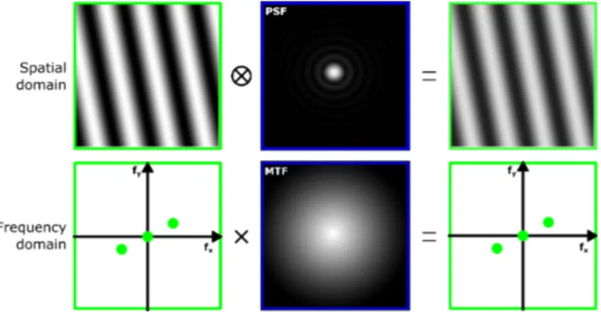
Figure 7: Image formation of a low (in green) and a high (in red) frequency modulation pattern using the concept of Fourier optics in spatial domain. The illumination is incoherent and the imaging system, aberration-free. The imaging system resolves the two sinusoidal object patterns. However, the contrast of the resulting image of the higher-frequency pattern is reduced.

Figure 8: Image formation of a low frequency modulation pattern using the concept of Fourier optics in spatial domain and in frequency domain. The illumination is incoherent and the imaging system, aberration-free. The imaging system resolves the sinusoidal object pattern. However, the contrast of the resulting image is reduced by the point spread function (in spatial domain) or the modulation transfer function (in frequency domain).

Figure 9: Image formation of a high frequency modulation pattern using the concept of Fourier optics in frequency domain. The illumination is incoherent (top of the figure) and coherent (bottom of the figure) and the imaging system, aberration-free. The incoherent imaging system resolves the sinusoidal object pattern but the contrast of the resulting image is reduced by the modulation transfer function, whereas the coherent imaging system is not able to transmit the features of the object pattern.