HAL Id: hal-00328247
https://hal.archives-ouvertes.fr/hal-00328247
Submitted on 23 Nov 2007HAL is a multi-disciplinary open access
archive for the deposit and dissemination of sci-entific research documents, whether they are pub-lished or not. The documents may come from teaching and research institutions in France or abroad, or from public or private research centers.
L’archive ouverte pluridisciplinaire HAL, est destinée au dépôt et à la diffusion de documents scientifiques de niveau recherche, publiés ou non, émanant des établissements d’enseignement et de recherche français ou étrangers, des laboratoires publics ou privés.
Intercomparison of UV-visible measurements of ozone
and NO2 during the Canadian Arctic ACE validation
campaigns: 2004–2006
A. Fraser, Florence Goutail, K. Strong, P. F. Bernath, C. Boone, W. H. Daffer,
J. R. Drummond, D. G. Dufour, T. E. Kerzenmacher, G. L. Manney, et al.
To cite this version:
A. Fraser, Florence Goutail, K. Strong, P. F. Bernath, C. Boone, et al.. Intercomparison of UV-visible measurements of ozone and NO2 during the Canadian Arctic ACE validation campaigns: 2004–2006. Atmospheric Chemistry and Physics Discussions, European Geosciences Union, 2007, 7 (6), pp.16283-16347. �hal-00328247�
ACPD
7, 16283–16347, 2007O3 and NO2 during the Canadian Arctic
ACE validation campaigns A. Fraser et al. Title Page Abstract Introduction Conclusions References Tables Figures ◭ ◮ ◭ ◮ Back Close Full Screen / Esc
Printer-friendly Version Interactive Discussion Atmos. Chem. Phys. Discuss., 7, 16283–16347, 2007
www.atmos-chem-phys-discuss.net/7/16283/2007/ © Author(s) 2007. This work is licensed
under a Creative Commons License.
Atmospheric Chemistry and Physics Discussions
Intercomparison of UV-visible
measurements of ozone and NO
2
during
the Canadian Arctic ACE validation
campaigns: 2004–2006
A. Fraser1, F. Goutail2, K. Strong1, P. F. Bernath3,4, C. Boone4, W. H. Daffer5, J. R. Drummond6,1, D. G. Dufour7, T. E. Kerzenmacher1, G. L. Manney8,9, C. T. McElroy10,1, C. Midwinter1, C. A. McLinden10, F. Nichitiu1, C. R. Nowlan1, J. Walker1, K. A. Walker1,4, H. Wu1, and J. Zou1
1
Department of Physics, University of Toronto, Toronto, Canada
2
Service d’A ´eronomie du Centre Nationale de la Recherche Scientifique, Verri `eres le Buisson, France
3
Department of Chemistry, University of York, Heslington, UK
4
Department of Chemistry, University of Waterloo, Waterloo, Canada
5
Columbus Technologies and Services Inc., Pasadena, USA
6
Department of Physics and Atmospheric Science, Dalhousie University, Halifax, Canada
7
Picomole Instruments Inc., Edmonton, Canada
8
Jet Propulsion Laboratory, California Institute of Technology, Pasadena, USA
ACPD
7, 16283–16347, 2007O3 and NO2 during the Canadian Arctic
ACE validation campaigns A. Fraser et al. Title Page Abstract Introduction Conclusions References Tables Figures ◭ ◮ ◭ ◮ Back Close Full Screen / Esc
Printer-friendly Version Interactive Discussion
9
New Mexico Institute of Mining and Technology, Socorro, USA
10
Environment Canada, Downsview, Canada
Received: 25 October 2007 – Accepted: 8 November 2007 – Published: 23 November 2007 Correspondence to: A. Fraser ([email protected])
ACPD
7, 16283–16347, 2007O3 and NO2 during the Canadian Arctic
ACE validation campaigns A. Fraser et al. Title Page Abstract Introduction Conclusions References Tables Figures ◭ ◮ ◭ ◮ Back Close Full Screen / Esc
Printer-friendly Version Interactive Discussion
Abstract
The first three Canadian Arctic ACE validation campaigns were held during polar sun-rise at Eureka, Nunavut, Canada (80◦N, 86◦W) from 2004 to 2006 in support of val-idation of the ACE (Atmospheric Chemistry Experiment) satellite mission. Three or four zenith-sky viewing UV-visible spectrometers have taken part in each of the three 5
campaigns. The differential slant column densities and vertical column densities from these instruments have been compared following the methods of the UV-visible Work-ing Group of the NDACC (Network for Detection of Atmospheric Composition Change). The instruments are found to partially agree within the required accuracies for both species, although both the vertical and slant column densities are more scattered than 10
required. This might be expected given the spatial and temporal variability of the Arctic stratosphere in spring. The vertical column densities are also compared to integrated total columns from ozonesondes and integrated partial columns from the ACE-FTS (ACE-Fourier Transform Spectrometer) and ACE-MAESTRO (ACE-Measurements of Aerosol Extinction in the Stratosphere and Troposphere Retrieved by Occultation) in-15
struments on board ACE. For both species, the columns from the ground-based instru-ments and the ozonesondes are found to generally agree within their combined error bars. The ACE-FTS ozone partial columns and the ground-based total columns agree within 4.5%, averaged over the three campaigns. The ACE-MAESTRO ozone partial columns are generally smaller than those of the ground-based instruments, by an av-20
erage of 9.9%, and are smaller than the ACE-FTS columns by an average of 14.4%. The ACE-FTS NO2 partial columns are an average of 13.4% smaller than the total columns from the ground-based instruments, as expected. The ACE-MAESTRO NO2 partial columns are larger than the total columns of the ground-based instruments by an average of 2.5% and larger than the partial columns of the ACE-FTS by an average 25
of 15.5%.
ACPD
7, 16283–16347, 2007O3 and NO2 during the Canadian Arctic
ACE validation campaigns A. Fraser et al. Title Page Abstract Introduction Conclusions References Tables Figures ◭ ◮ ◭ ◮ Back Close Full Screen / Esc
Printer-friendly Version Interactive Discussion
1 Introduction
The first three Canadian Arctic ACE (Atmospheric Chemistry Experiment) validation campaigns (the “Eureka campaigns”) were held during polar sunrise at the Polar En-vironmental Atmospheric Research Laboratory (PEARL), 15 km from Eureka, Nunavut (80◦N, 86◦W) from 2004 to 2006. In 2004 and 2005, the lab was known as AStrO 5
– the Arctic Stratospheric Ozone Observatory. All campaigns have involved a suite of six to seven ground-based instruments, including three to four zenith-viewing UV-visible spectrometers. In 2004, these UV-UV-visible instruments were: the University of Toronto Ground-Based Spectrometer (UT-GBS), the ground-based copy of the ACE-MAESTRO (ACE-Measurements of Aerosol Extinction in the Stratosphere and Tropo-10
sphere Retrieved by Occultation) instrument onboard ACE, and the SunPhotoSpec-trometer (SPS). In 2005 a Syst `eme d’Analyse par Observations Z ´enithales (SAOZ) instrument was added to the instrument suite. Detailed comparisons of the differen-tial slant column densities (DSCDs) and vertical column densities (VCDs) of ozone and NO2measured by these four instruments have been performed and are discussed
15
herein. These ground-based measurements are compared to partial columns mea-sured by the ACE-FTS (ACE-Fourier Transform Spectrometer) and ACE-MAESTRO instruments onboard the ACE satellite. The behaviour of the ozone and NO2columns with repect to the location of the polar vortex is also discussed.
The zenith-sky DSCDs and VCDs are compared following the protocols established 20
by the UV-visible Working Group of the Network for the Detection of Atmospheric Com-position Change (NDACC) (Kurylo and Zander, 2000). In order to maintain the uni-formity of measurements made throughout the NDACC, intercomparison campaigns between UV-visible instruments are periodically held. Three such campaigns have been held to date: in 1992 at Lauder, New Zealand (Hofmann et al., 1995), in 1996 25
at the Observatoire de Haute Provence, France (Roscoe et al.,1999), and in 2003 at the Andøya Rocket Range in Andenes, Norway (Vandaele et al.,2005). Roscoe et al.
(1999) andVandaele et al.(2005) present two methods of statistically comparing data 16286
ACPD
7, 16283–16347, 2007O3 and NO2 during the Canadian Arctic
ACE validation campaigns A. Fraser et al. Title Page Abstract Introduction Conclusions References Tables Figures ◭ ◮ ◭ ◮ Back Close Full Screen / Esc
Printer-friendly Version Interactive Discussion from two zenith-viewing instruments, which have been adopted by the UV-visible
Work-ing Group for the validation of new instruments (Johnston et al.,1999). Although the Canadian Arctic ACE Validation Campaigns were not NDACC intercomparison cam-paigns, they did meet the requirements of an instrument intercomparison: the mea-surement site was reasonably free from tropospheric pollution, meamea-surements were 5
made for at least ten days, measurements were taken over the the course of the entire day, and the measurements were coincident in time.
2 Description of the campaigns
The 2004 Canadian Arctic ACE Validation Campaign took place from 19 February to 15 April. Three UV-visible instruments (UT-GBS, MAESTRO, and SPS) were operated 10
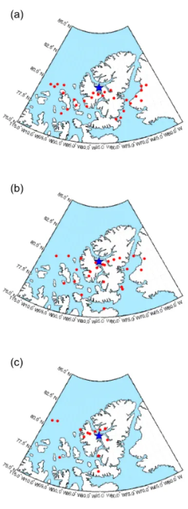
during the intensive phase, 19 February to 8 March. Only the UT-GBS remained for the extended phase of the campaign. Figure1a shows the ECMWF (European Centre for Medium-Range Weather Forecasts) potential vorticity (PV) map at a potential tem-perature of 475 K (∽19 km) for 4 March. This level is in the lower stratosphere, where the peak in ozone mixing ratio is located. 2004 was an unusual winter in the Arctic 15
stratosphere, with a sudden stratospheric warming occuring in December 2003. The vortex began to recover in February, and reformed with a strong vortex in the middle and upper stratosphere. The vortex in the lower stratosphere did not recover substan-tially, as seen in Fig. 1a. The stratosphere did not undergo a final warming until late April (Manney et al., 2005, 2007a). Eureka was inside the vortex at those altitudes 20
where it had reformed. The vertical columns from the intensive phase of this campaign have been previously discussed byKerzenmacher et al.(2005).
The 2005 campaign ran from 18 February to 31 March. Four UV-visible instruments (UT-GBS, SAOZ, MAESTRO, and SPS) were operated during the intensive phase, with measurements beginning on 18 February and continuing to 8 March. during the 25
extended phase, from 9 March to 31 March, only SAOZ and the UT-GBS remained in Eureka. The 2005 Arctic winter was notable for having the coldest stratospheric
ACPD
7, 16283–16347, 2007O3 and NO2 during the Canadian Arctic
ACE validation campaigns A. Fraser et al. Title Page Abstract Introduction Conclusions References Tables Figures ◭ ◮ ◭ ◮ Back Close Full Screen / Esc
Printer-friendly Version Interactive Discussion temperatures on record. A major final warming of the stratosphere occured on 10
March (Manney et al., 2007a). Figure 1b shows the ECMWF PV map at 475 K for 4 March. Eureka was on the edge of the polar vortex until early March, when the vortex began to move away and break apart.
The 2006 campaign took place from 17 February to 31 March. The same four UV-5
visible instruments as in 2005 were operated during both the intensive and extended phases of the campaign. 2006 was a warm winter in the polar stratosphere, with a sudden stratospheric warming occuring in January. As in 2004, the vortex began to reform in February, with a strong vortex (though not as strong as 2004) in the middle and upper stratosphere, and no substantial vortex in the lower stratosphere, as seen in 10
Fig.1c. The final warming of the stratosphere occured in April (Manney et al.,2007a). As in 2004, Eureka was inside the vortex at altitudes where it had reformed.
A more complete view of the synoptic context of the three campaigns can be found inManney et al.(2007a).
3 Instruments
15
The UT-GBS was assembled in 1998 and has since participated in seven polar sunrise campaigns at AStrO/PEARL (1999–2001, 2003–2007) (Bassford et al.,2005;Farahani,
2006; Farahani et al., 20071). It consists of a triple-grating spectrometer with a thermo-electrically cooled, back-illuminated, 2048×512 pixel CCD (charged-coupled device) array detector. In 2004, an older CCD was used, which was 2000×800 pixels. Sunlight 20
from the zenith-sky is gathered by a fused silica lens with a two-degree field-of-view, and focused on a liquid light guide, which minimises the effects of polarisation. Spectra are recorded continuously throughout the day, with varying exposure times to maximise the signal on the detector. Spectra were recorded between 345 and 560 nm, with a
1
Farahani, E., Strong, K., Mittermeier, R. L., and Fast, H.: Ground-based UV-visible spec-troscopy of O3, NO2, and OClO at Eureka: Part I – Evaluation of the analysis method and comparison with infrared measurements, Atmos. Chem. Phys. Discuss., in preparation, 2007.
ACPD
7, 16283–16347, 2007O3 and NO2 during the Canadian Arctic
ACE validation campaigns A. Fraser et al. Title Page Abstract Introduction Conclusions References Tables Figures ◭ ◮ ◭ ◮ Back Close Full Screen / Esc
Printer-friendly Version Interactive Discussion resolution of approximately 0.7 nm in the NO2 region (400–450 nm) and 1.1 nm in the
ozone region (450–550 nm). In 2004, an error in the data acquisition software caused a low signal-to-noise ratio, however, good data were still obtained. This error was corrected before the 2005 campaign. Also in 2004, data is missing between 15–23 and 25–29 of March due to a broken shutter in the spectrometer. The instrument is 5
installed in a viewing hatch inside PEARL, under UV-transmitting plexiglas.
The SAOZ instrument was constructed in the late 1980s, and is now deployed in a global network for measurements of stratospheric concentrations of trace gases im-portant to ozone loss (Pommereau and Goutail,1988). SAOZ spectra were recorded between 270 and 620 nm, with a resolution of 1.0 nm. The detector is an uncooled 10
1024-pixel linear diode array. SAOZ records zenith-sky spectra with a ten-degree field-of-view. Spectra are recorded every fifteen minutes throughout the day, and continu-ously during twilight, defined as when the solar zenith angle (SZA) is between 80◦and 95◦. SAOZ is installed in a viewing hatch under a UV-transmitting plexiglas window. A SAOZ instrument has taken part in all three NDACC intercomparison campaigns. 15
MAESTRO is the ground-based clone of the grating spectrometer on board ACE (McElroy et al., 2007). MAESTRO is a double spectrometer, with two independent input optics, gratings, and detectors. The UV spectrometer has a spectral range from 260 to 560 nm and a resolution of 1.0 nm. The visible spectrometer has a spectral range from 525 to 1010 nm and a resolution of 2.0 nm. Both detectors are uncooled 20
1024-pixel linear diode arrays. The field-of-view is 0.1◦ by 6.5◦. Only data from the UV spectrometer are used in this work.
SPS is the heritage instrument for MAESTRO. It is a photodiode array grating spec-trometer that has been flown aboard the NASA ER-2 aircraft as the Composition and Photodissociative Flux Measurement (CPFM) experiment (McElroy,1995). Zenith-sky 25
spectra are recorded between 375 and 775 nm, with a resolution of 1.5 nm in both the ozone and NO2 regions. The detector is an uncooled 1024-pixel linear photodiode ar-ray. Sunlight is collected by an achromatic lens, providing a 0.1◦ by 10◦ field-of-view. Although both MAESTRO and SPS are operated in direct Sun mode as well as
ACPD
7, 16283–16347, 2007O3 and NO2 during the Canadian Arctic
ACE validation campaigns A. Fraser et al. Title Page Abstract Introduction Conclusions References Tables Figures ◭ ◮ ◭ ◮ Back Close Full Screen / Esc
Printer-friendly Version Interactive Discussion sky mode, only the zenith-sky measurements will be discussed here. MAESTRO and
SPS are mounted on a solar tracker on the roof of PEARL, which tracks the Sun in az-imuth during zenith-sky viewing and in elevation and azaz-imuth during direct Sun viewing. The instruments are outside, and are operated at near ambient temperature (generally between −30◦C and −40◦C).
5
The ACE satellite, also known as SCISAT-1, is a solar occultation satellite launched by the Canadian Space Agency in August 2003 (Bernath et al.,2005). The goal of the ACE mission is to improve the understanding of the chemical and dynamical processes that control the concentrations of ozone in the middle atmosphere. Two instruments make up the payload: the ACE-FTS and ACE-MAESTRO. ACE-FTS is an infrared 10
Fourier transform spectrometer, with high resolution (0.02 cm−1), operating from 750– 4400 cm−1(Bernath et al.,2005). The version 2.2 data set including updates for ozone, HDO, and N2O5 is used here (Boone et al.,2005). ACE-MAESTRO is a UV-visible-near-IR double spectrometer, with a resoluton of 1.5–2.5 nm, and a wavelength range of 270–1040 nm. Version 1.2 is used here (McElroy et al., 2007). Only overpasses 15
within 500 km of Eureka are considered; the distance is determined using the location of the occultation at the 30 km tangent point. Figure2shows the location of the satellite overpasses used in the comparisons. All of the overpasses are sunset occultations.
Ozonesondes are launched weekly at the Eureka weather station (Tarasick et al.,
2005). During the intensive phase of all three campaigns, ozonesondes were launched 20
daily. Generally the ozonesondes are launched at 23:15 UTC (18:15 LT), however, on occasion, the launch time was altered to match a satellite overpass.
4 Data analysis and comparison method
4.1 Differential optical absorption spectroscopy
In this work, the DOAS technique (Differential Optical Absorption Spectroscopy) (e.g., 25
Solomon et al., 1987; Platt, 1994) is used for the analysis of spectra from all four 16290
ACPD
7, 16283–16347, 2007O3 and NO2 during the Canadian Arctic
ACE validation campaigns A. Fraser et al. Title Page Abstract Introduction Conclusions References Tables Figures ◭ ◮ ◭ ◮ Back Close Full Screen / Esc
Printer-friendly Version Interactive Discussion instruments with absorption cross-sections of ozone (Burrows et al.,1999), NO2(
Van-daele et al.,1998), H2O (converted from the line parameters given inRothman et al.,
2003), O4(Greenblatt et al.,1990), and the Ring pseudo-absorber (Chance and Spurr,
1997) fitted using a Marquardt-Levenberg non-linear least-squares technique. DSCDs of ozone are retrieved between 450 and 550 nm, and NO2 DSCDs are retrieved
be-5
tween 400 and 450 nm.
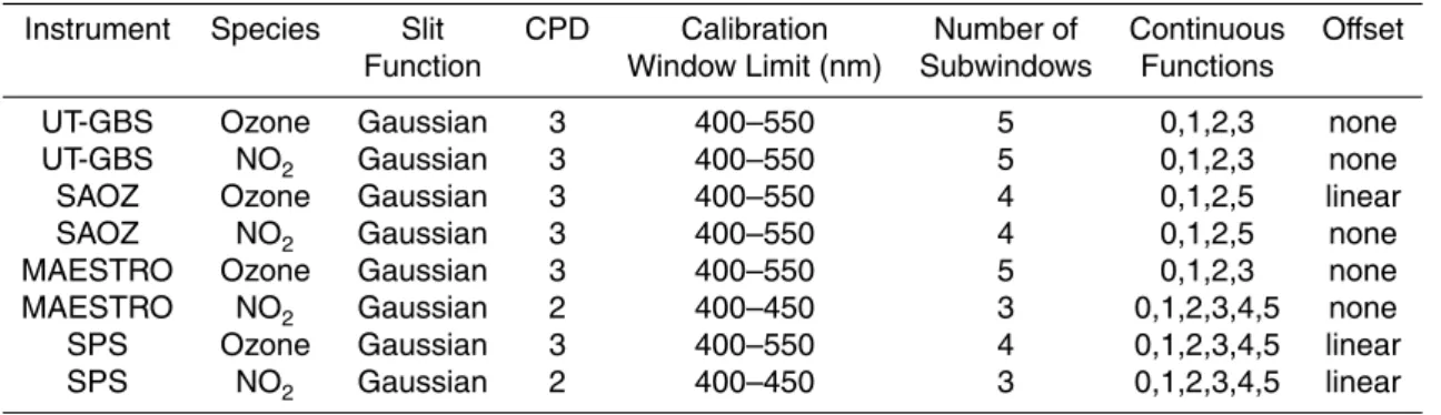
The program WinDOAS, developed by IASB-BIRA (Belgian Institute for Space Aeronomy, Fayt and Van Roozendael, 2001), has been used to analyse data from all four instruments. In this way, differences in the DSCDs should be a result of the spectra themselves and not an artefact of different analysis procedures. Table 1 gives 10
the details of the WinDOAS settings used for the four instruments. These settings were chosen to optimise the fits from the instruments. The Gaussian slit function is fit in each of the calibration subwindows and is used to smooth the high-resolution cross-sections to the resolution of the instrument. The wavelength calibration is performed on both the reference and twilight spectra. The degree of the polynomial fit to the optical depth 15
in the DOAS analysis is given by the continuous function. To correct for stray light in the instrument, an offset can be fit.
Daily reference spectra were used, with SZAs varying from 90.8◦ for the earliest day of the campaign (20 February) to 70.3◦for the last day of the campaign (14 April). If the reference spectra of two instruments differ by more than 0.5◦that day was not included
20
in the comparisons. This eliminated fewer than five comparisons from each campaign. Figure 3 shows typical ozone spectral fits from the four instruments for 4 March 2005. Figure 4 shows typical NO2 spectral fits for the same day. Fits from all years are comparable for all instruments. For both species, the MAESTRO spectral fits are noisier than those from the other instruments. This is because the other instruments 25
average spectra before they are analysed. For the UT-GBS and SAOZ, the number of spectra that are averaged is variable (4–300 for the UT-GBS, 1–115 for SAOZ), and is limited by the maximum time taken to record the spectra, to avoid smearing over large SZAs. SPS averages two spectra before they are analysed. MAESTRO
ACPD
7, 16283–16347, 2007O3 and NO2 during the Canadian Arctic
ACE validation campaigns A. Fraser et al. Title Page Abstract Introduction Conclusions References Tables Figures ◭ ◮ ◭ ◮ Back Close Full Screen / Esc
Printer-friendly Version Interactive Discussion records individual spectra. In this work, MAESTRO DSCDs are averaged over 0.25◦
intervals. Individual integration times range between 13 ms and 30 s for the UT-GBS, between 0.5 s and 19 s for SAOZ, and between 50 ms and 10 s for MAESTRO and SPS. The NO2 DOD fits for SPS and MAESTRO are poorer than the fits from the UT-GBS and SAOZ. The Eureka campaigns take place just after polar sunrise, when the NO2
5
column is very small. The NO2is near the limits of detection of SPS and MAESTRO. 4.2 Derivation of vertical column densities
The primary quantity derived from the zenith-sky measurements is the DSCD as a function of solar zenith angle. In order to convert the measurements of DSCD into VCD, the use of an air mass factor is required. In this work, daily air mass factors (AMFs) are 10
calculated using a radiative transfer model initialized with temperature, pressure, and ozone profiles taken from the ozonesondes flown on that day and NO2profiles taken from a chemical box model at 75◦N in February or March (McLinden et al.,2002). If no ozonesonde is available, the nearest sonde to that day is taken. NO2 is allowed to vary along the path of light, using the diurnal variation from the chemical box model. 15
DSCDs are related to the VCD and the AMF by Eq. (1):
DSCD(SZA)=VCD(SZA) × AMF(SZA)−RCD. (1)
RCD is the reference column density, and is the amount of absorber in the reference spectrum used in the DOAS analysis.
Two methods are used to convert ozone DSCDs to VCDs. In the first method, or 20
Langley plot method, a Langley plot of DSCD between 86◦ and 91◦ versus AMF is made. From Eq. (1), the VCD can be found by finding the slope of the Langley plot. The Langley plot will only be a straight line if the AMFs are correct, if the ozone is constant through the twilight period, and if the ozone field is homogenous. In the second method, or averaging method, a Langley plot of DSCD between 86◦ and 91◦ 25
versus AMF is made. From Eq. (1), the RCD can be found by taking the ordinate of the Langley plot. The RCDs from the morning and afternoon are averaged to give one
ACPD
7, 16283–16347, 2007O3 and NO2 during the Canadian Arctic
ACE validation campaigns A. Fraser et al. Title Page Abstract Introduction Conclusions References Tables Figures ◭ ◮ ◭ ◮ Back Close Full Screen / Esc
Printer-friendly Version Interactive Discussion RCD for each day. Each individual DSCD is then converted to a VCD using Eq. (1).
The average VCD for one twilight period is found by averaging the VCDs between 86◦ and 91◦. The two methods should yield the same results, provided the Langley plot is a straight line (Sarkissian et al.,1997).
There are also two methods to convert NO2DSCDs to VCDs. The averaging method
5
can be used, or the VCD at 90◦can be found using the DSCD at 90◦and Eq. (1). The RCD is found by making a Langley Plot of DSCDs between 86◦ and 91◦. Ideally, SZAs from 80◦ to 85◦ would be used, but these are not available for many days during the campaigns. The RCDs from both twilight periods are averaged to give a daily RCD. For NO2, the results from each method are slightly different, due to the diurnal variation of 10
NO2, with the averaging method yielding an average VCD between 86◦ and 91◦, and the 90◦method yielding a VCD at 90◦.
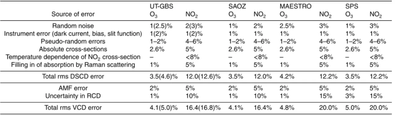
Measurement errors are calculated from the root-sum-square (rms) of individual sources of error, after Bassford et al. (2005) and references therein. For DSCDs, they include random noise on the spectra, instrument error arising from uncertain-15
ties in the dark current, bias, and slit function, pseudo-random errors resulting from unaccounted-for structure in the spectra, errors in the absorption cross-sections, the temperature dependence of the NO2cross section, and the effects of multiple Raman scattering, which fills in the absorption lines. For VCDs, they also include error in the air mass factors and uncertainty in the reference column density. The individual and 20
total errors are shown in Table 2. 4.3 Comparison methods
The ground-based instruments are all zenith-viewing, and therefore share the same viewing geometry, although not the same field-of-view. The DSCDs can be com-pared as described in Johnston et al. (1999). Two types of certification are defined 25
by NDACC. Type 1 standards apply to instruments that are certified for global studies and trend measurements. The DSCDs from two instruments are transformed onto a common SZA grid ranging from 75◦ to 91◦, and then a linear regression analysis is
ACPD
7, 16283–16347, 2007O3 and NO2 during the Canadian Arctic
ACE validation campaigns A. Fraser et al. Title Page Abstract Introduction Conclusions References Tables Figures ◭ ◮ ◭ ◮ Back Close Full Screen / Esc
Printer-friendly Version Interactive Discussion performed. In this work, on days when the Sun did not reach 75◦, the minimum SZA
was used. The slope of the regression fit represents how well the two data sets agree: a non-unity slope indicates that the DSCDs diverge. A non-zero ordinate represents a systematic offset between the two data sets. Residuals are also calculated. Large residuals are a sign of scatter in at least one of the data sets. The linear regressions 5
are performed following the method of York et al. (2003), which is a least-squares estimation method. The following targets have been set for the campaign mean of these parameters: slope = (0.97–1.03), intercept = ±55.8 DU (Dobson Units), and root-mean-square of the residuals <37.2 DU for ozone and slope = (0.95–1.05), inter-cept = ±1.5×10¹⁵molec/cm2, and residuals <1.0×10¹⁵molec/cm2for NO2. An exam-10
ple of the Type 1 regression analysis is shown in Fig.5for 4 March 2005 between the UT-GBS and SAOZ.
Instruments that meet Type 2 standards are certified for process studies and satellite validation. In this comparison, the VCDs over the course of a twilight are transformed onto a common SZA grid ranging from 85◦to 91◦ and the mean of the ratio of the data 15
from the two instruments is taken. For ozone, the campaign mean of the ratio should be between 0.95 and 1.05, with a standard deviation (one sigma) less than 0.03. For NO2, the mean of the ratio should be between 0.90 and 1.10, with a standard deviation (one sigma) less than 0.05. Figure6shows an example of this comparison for 4 March 2005 between the UT-GBS and SAOZ. Since NO2 has a diurnal variation, the offset
20
between the morning and afternoon VCDs can be calculated by finding the y-intercept of a plot of the afternoon VCDs against the morning VCDs. If the diurnal variation of the species is roughly constant over the campaign, the standard deviation in this offset over the duration of the campaign should be less than 2.5×10¹⁵molec/cm2. However, for polar measurements, the amount of sunlight varies significantly from day to day, 25
meaning the diurnal variation is not constant, and so the offset is not expected to be constant. Because of this, the offset is not discussed herein.
ACPD
7, 16283–16347, 2007O3 and NO2 during the Canadian Arctic
ACE validation campaigns A. Fraser et al. Title Page Abstract Introduction Conclusions References Tables Figures ◭ ◮ ◭ ◮ Back Close Full Screen / Esc
Printer-friendly Version Interactive Discussion
5 Differential slant column density comparisons
5.1 Ozone
Figure7 shows the DSCDs for the five ground-based instruments on 4 March 2004– 2006. The general agreement between all the instruments is good up to 92◦. At this point the MAESTRO and SAOZ DSCDs begin to diverge from the other instruments. 5
In the case of SAOZ, the divergence is always to lower DSCDs. This divergence is due to the warm temperatures inside the viewing hatch of the instrument. Thermal noise increases as the detector gets warmer, and the data beyond 92◦is unreliable as a result. The MAESTRO DSCDs diverge to both higher and lower DSCDs, depending on the twilight period. There seems to be no relation between which way the DSCDs 10
diverge and the outside temperature or cloudiness of the day. As only SZAs up to 91◦ are used in the DSCD comparisons and in the calculation of VCDs, these divergences will not affect the comparisons to be discussed.
Figure 8shows the results of the Type 1 ozone DSCD comparisons. In all figures, the campaign-averaged parameter is given, with the standard error (σ/√N, σ is the 15
standard deviation, N is the number of comparisons) represented as the error bars. Table 3 gives the number of twilight periods averaged in each of the comparisons. No MAESTRO vs. SPS comparison is given for the 2004 campaign due to the small number of twilight periods available for comparison (less than three).
Examining the slopes first, 16 of the 28 values (seen in Fig. 8a, d, and g) meet the 20
NDACC standards, and a furthur three meet the standards within the error bars. The comparisons in 2004 and 2006 are similar, with the exception of the UT-GBS vs. SPS afternoon comparisons. It should be noted that the 2004 comparison has only three data points. The NDACC requires at least ten days of comparisons to ensure proper statistics. The comparisons tend to be worse in 2005, especially the UT-GBS vs. SAOZ 25
comparison. As discussed in Sect.2, Eureka was located on the edge of the polar vor-tex throughout most of the campaign. SAOZ has a significantly larger field-of-view than the UT-GBS (10◦vs. 2◦). Because of this, SAOZ will view more of the atmosphere than
ACPD
7, 16283–16347, 2007O3 and NO2 during the Canadian Arctic
ACE validation campaigns A. Fraser et al. Title Page Abstract Introduction Conclusions References Tables Figures ◭ ◮ ◭ ◮ Back Close Full Screen / Esc
Printer-friendly Version Interactive Discussion the UT-GBS. With the heterogenous ozone field expected due to Eureka’s position
on the edge of the vortex, the discrepancy in DSCDs is likely a result of the instru-ments sampling different portions of the atmosphere. The sizes of the fields-of-view of MAESTRO and SPS are between those of the UT-GBS and SAOZ, so the effect is not expected to be as large. No pairs of instruments meet the NDACC standards for 5
both twilight periods in all years of comparison, however the UT-GBS vs. SAOZ com-parisons consistently do not meet the slope standards. The UT-GBS vs. MAESTRO comparisons meet the NDACC standards within the error bars each year; the only twi-light period that does not meet the standards is the 2005 afternoon, where there are just seven days to compare. Generally, comparisons with SPS and MAESTRO improve 10
in 2006 when these instruments participated in the extended phase of the campaign. For the average intercepts, in Fig.8b, e, and h 23 of the 28 comparisons meet the NDACC standards, and a further four comparisons agree within the error bars. For comparisons involving SPS and MAESTRO, the standard errors are large compared to the average intercepts. The UT-GBS vs. SAOZ, UT-GBS vs. SPS, and SPS vs. SAOZ 15
comparisons consistently meet the NDACC standard for both twilight periods for all years of comparison. The average residuals (Fig. 8c, f, and i) are all much larger than the NDACC standard, with large standard error, with the exception of the UT-GBS vs. SAOZ 2006 comparison. As discussed in Sect.4.3, large residuals are an indication of scatter in at least one of the data sets.
20
The campaign-averaged results of the Type 2 ozone comparisons are shown in Fig. 9. In 2004 and 2006, most of the ratios agree with the NDACC standards, or are slightly outside the range (e.g. the SPS vs. SAOZ 2006 comparisons). In 2005, the UT-GBS vs. SAOZ, UT-GBS vs. MAESTRO, SPS vs. SAOZ, and MAESTRO vs. SPS comparisons are all outside the range, although some of these comparisons agree 25
within the error bars. In Fig.8, the corresponding comparisons generally have slopes that do not meet the NDACC standards, and intercepts that do. As discussed above, this discrepancy may be due to Eureka’s position on the edge of the polar vortex during much of the campaign, and the difference in fields-of-view of the instruments.
ACPD
7, 16283–16347, 2007O3 and NO2 during the Canadian Arctic
ACE validation campaigns A. Fraser et al. Title Page Abstract Introduction Conclusions References Tables Figures ◭ ◮ ◭ ◮ Back Close Full Screen / Esc
Printer-friendly Version Interactive Discussion The standard deviations of the ratios for the campaign are also shown in Fig. 9.
Most of the standard deviations are larger than the requirement, the exceptions be-ing the UT-GBS vs. SAOZ comparisons for all years, the UT-GBS vs. MAESTRO 2004 comparison, the morning of the UT-GBS vs. SPS 2004 comparison, and the morning of the SPS vs. SAOZ 2005 comparison. This is an indication of the consistency of the 5
ratio comparisons – small standard deviations mean that the ratio has a smaller spread of values. The standard deviations for comparisons involving SPS and MAESTRO are, in general, larger in 2006 than in 2005. This is likely a result of these instruments par-ticipating in the extended campaign. As the light levels increased towards the end of March, both instruments recorded many more saturated spectra than during the inten-10
sive phase. As a result there are fewer DSCDs for these instruments. The regression parameters for comparisons involving MAESTRO and SPS during the extended phase are more scattered than during the intensive phase. If only the intensive phase is considered, the standard deviations are smaller.
5.2 NO2
15
Figure10shows the NO2DSCDs from the four ground-based instruments for 4 March 2004–2006 (the same day as in Fig. 7). The UT-GBS DSCDs from 2004 are much more scattered than those in the other years, as a result of the low signal-to-noise ratio discussed in Sect.3. In all years, there is more scatter in the data, and a greater discrepancy is seen between the instruments than for the ozone DSCDs. In 2004, the 20
SPS and MAESTRO DSCDs are roughly the same at noon, and are within the large scattered range of the UT-GBS. At high SZAs, the DSCDs from the three instruments diverge. In 2005–2006, the agreement between all instruments is good at lower SZAs, and the DSCDs begin to diverge at higher SZAs. The MAESTRO and SPS DSCDs are more scattered than those of the other instruments for all SZAs. In 2005, the UT-25
GBS and SAOZ DSCDs agree, while the SPS and MAESTRO DSCDs are smaller. In 2006, the DSCDs from SPS and MAESTRO are scattered about the DSCDs from the UT-GBS and SAOZ. The SAOZ DSCDs become scattered above 92◦, a result of the
ACPD
7, 16283–16347, 2007O3 and NO2 during the Canadian Arctic
ACE validation campaigns A. Fraser et al. Title Page Abstract Introduction Conclusions References Tables Figures ◭ ◮ ◭ ◮ Back Close Full Screen / Esc
Printer-friendly Version Interactive Discussion higher thermal noise contribution discussed in Sect.5.1. Only SZAs up to 91◦are used
in the comparisons.
Figure 11shows the results of the Type 1 comparisons for NO2 for the 2005–2006 campaigns. The error bars represent the standard errors. No comparisons are shown in 2004 due to the small number of comparisons for this year (less than three), as well 5
as the large amount of scatter on the DSCDs from the UT-GBS. No NO2comparisons from MAESTRO are shown in 2005 due to the small number of twilight periods available for comparison. The number of twilight periods used in the averages is given in Table 3. Eleven of the 16 campaign-averaged slopes agree with the NDACC standards, and an additional one agrees within error bars. The UT-GBS vs. SAOZ comparison meets 10
the standard for both twilight periods for both years of comparison. No pair of instru-ments consistently fails to meet the NDACC standards. In general, the standard errors of the morning slopes are larger than those of the afternoon slopes, a result of the smaller amount of NO2in the morning versus the afternoon.
For the campaign-averaged intercepts, 17 of the 18 comparisons meet the NDACC 15
standards, while the remaining comparison meets the standard within the error bars. As with the slope values, the standard errors are generally larger in the morning than in the afternoon. The campaign-averaged residuals for the UT-GBS vs. SAOZ compar-ison meet or are close to the NDACC standards in both years. The other residuals, however, are up to four times larger than the standard. This is a reflection of the scatter 20
in the DSCDs discussed above.
The results of the Type 2 NO2comparisons are shown in Fig.12. All but two of the ratio results meet the NDACC standard. One of these, the MAESTRO vs. SPS 2005 afternoon comparison, is very close with a large error bar. The other, the UT-GBS vs. SPS comparison, is large and does not agree within the error bars. The slope for 25
this pair in the Type 1 comparisons shown in Fig.11is also large.
The standard deviations of the ratios for the campaign are also shown in Fig. 12. All of the standard deviations are up to nine times the NDACC standard. This is a reflection of the scatter in the DSCDs, and hence the VCDs. The NDACC standards
ACPD
7, 16283–16347, 2007O3 and NO2 during the Canadian Arctic
ACE validation campaigns A. Fraser et al. Title Page Abstract Introduction Conclusions References Tables Figures ◭ ◮ ◭ ◮ Back Close Full Screen / Esc
Printer-friendly Version Interactive Discussion were established after a summer-time mid-latitude intercomparison campaign, when
NO2is at its annual peak. There is significantly less NO2in the polar springtime Arctic stratosphere, making it more difficult to detect, and therefore increasing the random noise (scatter) on the DSCDs.
5.3 Relation to the previous MANTRA 2004 comparison 5
The UT-GBS, SAOZ, MAESTRO, and SPS instruments all took part in the Middle Atmo-sphere Nitrogen TRend Assessment (MANTRA) campaign in Vanscoy, Saskatchewan (52◦N, 107◦W) in late summer 2004. The results from this comparison were discussed byFraser et al.(2007). For the MANTRA Type 1 ozone comparison, the slopes were found to agree with the NDACC standards for the MAESTRO vs. SPS comparisons. 10
The morning slopes for the UT-GBS vs. SPS and MAESTRO vs. SAOZ comparisons also met the NDACC standards. The UT-GBS vs. SPS afternoon and both UT-GBS vs. MAESTRO comparisons agreed with the standards within the standard error. The intercepts were universally large, two to four times the NDACC standards, with large standard error, and the residuals were large: up to three times the NDACC standard. 15
For the ozone Type 1 analysis for the Eureka campaigns, the slopes and residu-als found here are consistent with the slopes and residuresidu-als found during the MANTRA campaign. The intercepts for the Eureka campaigns are much smaller than those found during MANTRA. A daily reference spectrum was used for the DOAS analysis in the Eureka campaigns, while a single reference spectrum was chosen for the MANTRA 20
campaign. Daily reference spectra may cause more consistent intercepts since shifts in the wavelength calibration can occur over the course of a campaign for an instru-ment due to changes in the temperature. Since the diurnal changes in the wavelength calibration are in general smaller than the changes over a campaign, using a daily ref-erence spectrum can result in better calibration for the DOAS analysis, and thus more 25
accurate DSCDs at lower SZAs.
The MANTRA Type 2 ozone comparisons had the morning GBS vs. SAOZ, UT-GBS vs. MAESTRO, and morning MAESTRO vs. SAOZ ratios all meeting the NDACC
ACPD
7, 16283–16347, 2007O3 and NO2 during the Canadian Arctic
ACE validation campaigns A. Fraser et al. Title Page Abstract Introduction Conclusions References Tables Figures ◭ ◮ ◭ ◮ Back Close Full Screen / Esc
Printer-friendly Version Interactive Discussion standards, while the other comparisons were close to the desired range. The SPS
vs. SAOZ comparisons were significantly smaller than the standards. The standard deviations for all comparisons, with the exception of the UT-GBS vs. SAOZ morning, were within the standards. The ozone Type 2 ratios presented here are better than those found during the MANTRA campaign: the ratios mostly meet the NDACC stan-5
dards. The standard deviations are larger than during MANTRA, most likely due to the larger spatial and diurnal variability in the spring polar ozone field versus the summer mid-latitude ozone field.
Only NO2 data from the UT-GBS and SAOZ were presented inFraser et al.(2007). For the Type 1 comparisons, the slopes met the NDACC standards. The morning inter-10
cept was 3.5 times larger than required, while the afternoon intercept was 1.25 times larger than the standard. The residuals were three to four times larger. In the com-parisons for Eureka for the UT-GBS and SAOZ, all three parameters meet the NDACC standards in 2006. In 2005, only the afternoon residual does not meet the standard. The improved comparisons are a result of the improved signal-to-noise ratio of the UT-15
GBS after the MANTRA 2004 campaign, when the error in the data acquisition code was discovered and a new CCD was obtained.
For the Type 2 NO2 comparisons, the NDACC standards were met in the MANTRA comparison, with the exception of the morning standard deviation. In the Eureka com-parison, the ratios meet the NDACC standard, while the standard deviations do not. 20
This is likely due to low NO2 concentrations and atmospheric variability of the spring-time polar atmosphere.
6 Vertical column density comparisons
6.1 Comparison of methods
As discussed in Sect.4.2, there are two methods for calculating both the ozone and 25
NO2 vertical column densities. Figure13shows the results of both of these methods 16300
ACPD
7, 16283–16347, 2007O3 and NO2 during the Canadian Arctic
ACE validation campaigns A. Fraser et al. Title Page Abstract Introduction Conclusions References Tables Figures ◭ ◮ ◭ ◮ Back Close Full Screen / Esc
Printer-friendly Version Interactive Discussion for both species in 2005 for the UT-GBS instrument only. Both methods have been
used on the other four instruments as well, and the differences between the methods are similar. This year is shown because Eureka spent the beginning of the campaign on the edge of the polar vortex. After March 8 (day 67), the vortex moved away from Eureka and began to break up (Manney et al.,2007a).
5
The ozone results, shown in Fig.13a, show poor agreement between the two meth-ods to day 67, and good agreement between the VCDs after this day. The discrep-ancies between the methods can be as high as 50 DU (or ∽15% of the total column) during the first half of the campaign, while the differences are no greater than 20 DU (or ∽6% of the total column) during the second half. While Eureka was on the edge 10
of the vortex, due to the viewing geometry of the instrument, the air masses sampled in the morning were towards the east into the vortex, while the air masses sampled in the afternoon were towards the west, out of the vortex (see Fig.1). The SZA range used for both methods is 86◦ to 91◦. Both methods of finding the ozone VCD assume that the VCD does not change over the twilight period. This assumption is not valid for 15
the period that Eureka was on the edge of the vortex, because each DSCD is in fact sampled at a different physical location. The measurements closest to noon are south of Eureka, while those near a SZA of 90◦ are to the East or the West, either into the vortex in the morning or away from the vortex in the afternoon. Figure14 shows the geometrical projection of the ozone maximum (taken to be 18 km) along the line of sight 20
to the Sun for 4 March 2005. Because there are more measurements taken at solar noon, the averaging method weights the VCD towards these noontime measurements. For this period of the campaign, this results in larger VCDs in the morning and smaller VCDs in the afternoon. during the second part of the campaign, when the vortex had moved away from Eureka, the methods agree, as a result of the more homogenous 25
ozone field.
The NO2results, shown in Fig.13b, do not display the same dramatic differences in the methods as the ozone results. Unlike the total ozone column, the NO2column has a diurnal cycle, and its concentrations are expected to vary throughout the twilight period.
ACPD
7, 16283–16347, 2007O3 and NO2 during the Canadian Arctic
ACE validation campaigns A. Fraser et al. Title Page Abstract Introduction Conclusions References Tables Figures ◭ ◮ ◭ ◮ Back Close Full Screen / Esc
Printer-friendly Version Interactive Discussion The 90◦method takes this into account by finding the VCD at 90◦, while the averaging
method finds the average VCD between 86◦ and 91◦. However, both methods assume that the same air mass is viewed throughout the twilight period, which is not the case in the first part of the campaign when Eureka was on the edge of the polar vortex. The fact that the two methods agree during the whole campaign is an indication that 5
the NO2 field is not as heterogeneous as the ozone field. The VCDs become less scattered after 8 March, when the vortex moves away from Eureka.
6.2 Ozone VCDs 6.2.1 2004
The ozone vertical column densities calculated using the averaging method from all the 10
ground-based instruments for the Eureka 2004 campaign are shown in Fig.15a and b. The averaging method is selected to minimise the morning and afternoon differences, due to the weighting towards noon, discussed in Sect. 6.1. In addition, Sarkissian
et al. (1997) find the averaging method to better agree with ozonesondes. Also shown in Fig. 15b are integrated ozonesonde profiles. A correction has been added to the 15
ozonesonde columns to account for ozone above the balloon burst height. Errors on the ozonesonde total columns are 5% (Tarasick et al.,2005).
In the following discussions, the average percentage difference is calculated using Eq. (2):
P D= 100 ×
n
X
i
d ata1,i− d ata2,i
av eragei (2)
20
PD is the percentage difference, data1and data2are the two data sets being compared, average is the average of the two data sets, n is the number of days of comparison, and i is the day index.
In Fig. 15a, the morning VCDs of all three instruments (UT-GBS, SPS, and MAE-STRO) agree within error bars, and within an average of 2.4 DU (0.5%) to 4.4 DU 25
ACPD
7, 16283–16347, 2007O3 and NO2 during the Canadian Arctic
ACE validation campaigns A. Fraser et al. Title Page Abstract Introduction Conclusions References Tables Figures ◭ ◮ ◭ ◮ Back Close Full Screen / Esc
Printer-friendly Version Interactive Discussion (0.9%). In Fig. 15b, the afternoon VCDs of the three instruments agree within error
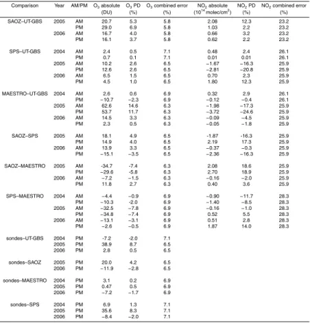
on most days and within 0.7 (0.1%) and 10.3 DU (2.0%) on average. During the entire campaign, the ozonesonde columns agree with the ground-based instruments within error on most days. The sonde columns agree within an average of 3.1 DU (0.2%) to 7.2 DU (2.0%) with the ground-based columns and tend to be slightly higher. The 5
campaign-averaged absolute and percentage differences for the ground-based instru-ments and the ozonesondes are given in Table 4. Also shown in this table is the combined percentage error in the VCDs from each pair of instruments compared. All the compared instruments agree within the combined errors.
Integrated partial columns from the ACE-FTS and ACE-MAESTRO profiles taken 10
within 500 km of Eureka are shown in Fig.16a, along with the average VCDs from the ground-based instruments. The partial columns were calculated by using the volume mixing ratio from the FTS and MAESTRO and the density from the ACE-FTS profiles. The ACE satellite overpasses are all in the afternoon, falling between 15:00 LT and 17:42 LT. All the overpasses correspond to SZAs of 89.5◦. For ozone, 15
the partial column is between 15 and 40 km. Kar et al. (2007) found these altitudes to be the region where ACE-MAESTRO data is appropriate for scientific analysis. The same altitude range is chosen for ACE-FTS to facilitate comparisons, especially with ACE-MAESTRO. For the ACE-FTS, Dupuy et al. (2007)2use a similar altitude region: 16–44 km. To account for the tropospheric ozone contribution below 15 km, the daily 20
ozonesonde data below this altitude have been added to the satellite columns. The column below 15 km is between 98 DU and 207 DU, or about 30%. The ozonesondes launched during the three campaigns have total columns ranging between 350 DU and 560 DU. Assuming an exponential decay in the ozone column above the burst height of the balloon, the contribution to the total column from 40 to 100 km is between 1 DU and 25
16 DU. On average, the column above 40 km is 2% of the total column. Since the error on all the columns is greater than 2%, the ground-based total columns and satellite
2
Dupuy, E., Walker, K. A., Kar, J., et al.: Validation of ozone measurements from the Atmo-spheric Chemistry Experiment (ACE), Atmos. Chem. Phys. Discuss., submitted, 2007.
ACPD
7, 16283–16347, 2007O3 and NO2 during the Canadian Arctic
ACE validation campaigns A. Fraser et al. Title Page Abstract Introduction Conclusions References Tables Figures ◭ ◮ ◭ ◮ Back Close Full Screen / Esc
Printer-friendly Version Interactive Discussion partial columns are expected to agree within error bars. A similar approach is used in
Randall et al.(2002).
The average afternoon ozone VCDs from the three ground-based instruments are also shown in Fig. 16a, along with the total columns from the ozonesondes and the partial columns from the satellite instruments. Only the period with satellite overpasses 5
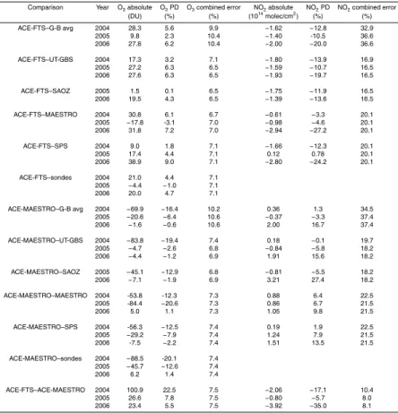
is shown. The ACE-FTS partial columns in Fig. 16a agree with the ground-based columns and sondes for most days. On average, the ACE-FTS partial columns agree with the four sets of ground-based VCDs within 9.0 DU (1.8%) to 30.8 DU (6.1%), and with the sondes within 21.0 DU (4.4%) (see column 4 of Table 5). The ACE-MAESTRO partial columns are generally smaller than those from the ground-based instruments 10
and sondes, and for the most part do not agree within error bars. On average, the ACE-MAESTRO partial columns agree within 53.8 DU (12.3%) to 83.8 DU (19.4%) with the ground-based and within 88.5 DU (20.1%) with the sonde columns. The ACE-FTS partial columns are larger than those of the ACE-MAESTRO, with the exception of days 55 and 70. The ACE-FTS columns are an average of 100.9 DU (22.5%) larger than the 15
ACE-MAESTRO columns. The absolute and percentage differences for the individual instrument comparisons with the satellite instruments are shown in Table 5, as well as the combined percentage error of each pair of instruments compared. For comparisons with ACE-FTS, all of the individual comparisons agree within the combined error of the two instruments. For comparisons with ACE-MAESTRO, the individual comparisons 20
do not agree within the combined error of the two instruments. 6.2.2 2005
Figure17a shows the morning ozone VCDs from the ground-based instruments for the Eureka 2005 campaign. The columns from the UT-GBS, SAOZ, and SPS all mostly agree within error bars. The MAESTRO columns are larger than those from the other 25
instruments, with the exception of day 65 (6 March). Generally, the MAESTRO columns do not agree with the other instruments within error bars. The UT-GBS, SAOZ, and SPS agree within 10.2 DU (2.6%) to 20.7 DU (5.3%), and these three instruments agree with
ACPD
7, 16283–16347, 2007O3 and NO2 during the Canadian Arctic
ACE validation campaigns A. Fraser et al. Title Page Abstract Introduction Conclusions References Tables Figures ◭ ◮ ◭ ◮ Back Close Full Screen / Esc
Printer-friendly Version Interactive Discussion MAESTRO within 32.5 DU (7.4%) to 62.6 DU (14.6%). The UT-GBS columns are the
smallest of the four instruments.
Figure17b shows the afternoon ozone VCDs from the ground-based instruments as well as the integrated columns from the sondes. As in the morning, the MAESTRO columns are larger than those from the other ground-based instruments, with the ex-5
ception of day 65. Again, the columns from the other three ground-based instruments mostly agree within error bars and agree within 12.6 DU (2.6%) to 29.0 DU (6.9%). The agreement with MAESTRO is between 29.6 DU (5.8%) and 53.7 DU (11.7%). The ozonesonde columns are higher than the ground-based columns, with the exception of MAESTRO, and mostly agree within error bars with SAOZ and the SPS. Half the 10
indivudual comparisons with the UT-GBS, and two-thirds of the individual compar-isons with MAESTRO do not agree within error bars. The sondes agree with the ground-based instruments between 0.47 DU (0.5%) and 38.9 DU (8.7%). Generally, the UT-GBS columns are the smallest of all the instruments. In Table 4, the individual comparisons agree within combined error, with the exception of the comparisons with 15
MAESTRO, the SAOZ–UT-GBS afternoon, and the sondes–UT-GBS comparisons. The average afternoon VCDs from the ground-based instruments are shown in Fig.18a, along with the total columns from the ozonesondes, and the partial columns from the satellite instruments. The ACE-FTS partial columns agree with the ground-based instruments and the sondes on most days of the campaign. On average, the 20
ACE-FTS columns agree with the ground-based instruments within 1.5 DU (0.1%) to 27.2 DU (6.3%), and with the sondes to 4.4 DU (1.0%). The agreement between the MAESTRO and the other instruments is improved this year. On average, the ACE-MAESTRO partial columns agree with the UT-GBS, SAOZ, and SPS between 4.7 DU (2.6%) and 45.1 DU (12.9%), and with the MAESTRO within 84.4 DU (20.6%). The 25
ACE-FTS columns are 26.6 DU (7.8%) larger than the ACE-MAESTRO columns. In Table 5, all the comparisons with ACE-FTS are within the combined percentage error of the individual instruments. The comparisons with ACE-MAESTRO are generally not within the combined percentage error.
ACPD
7, 16283–16347, 2007O3 and NO2 during the Canadian Arctic
ACE validation campaigns A. Fraser et al. Title Page Abstract Introduction Conclusions References Tables Figures ◭ ◮ ◭ ◮ Back Close Full Screen / Esc
Printer-friendly Version Interactive Discussion 6.2.3 2006
The morning ozone VCDs for the Eureka 2006 campaign are shown in Fig.19a. The ground-based instruments agree within error bars on most days. The MAESTRO and SPS columns are scattered about the SAOZ and UT-GBS columns, while the SAOZ columns are universally larger than those from the UT-GBS. On average, the instru-5
ments agree within 6.5 DU (1.5%) to 16.7 DU (4.0%).
Figure19b shows the afternoon VCDs from the 2006 campaign. During the intensive phase, the agreement between the ground-based instruments is similar to that of the morning columns, with the MAESTRO and SPS scattered about the SAOZ and UT-GBS columns. Again, the UT-GBS columns are universally smaller than those of the SAOZ. 10
Again, the columns mostly agree within error bars. On average, the ground-based instruments agree within 2.3 DU (0.5%) to 16.1 DU (3.7%). The agreement between the ozonesonde columns and the ground-based VCDs is also good, with the sonde columns being, on average, within 2.8 DU (0.5%) to 11.9 DU (2.8%). In Table 4, all the instrument comparisons agree within the combined percentage error.
15
The average total columns from the ground-based instruments, the total columns from the ozonesondes, and the partial columns from the satellite instruments, are shown in Fig.20a. As in 2004 and 2005, the ACE-FTS partial columns mostly agree within error bars with the total columns from the ground-based instruments and the ozonesondes. The agreement is, on average, between 19.5 DU (4.3%) and 38.9 DU 20
(9.0%) of the ground-based instruments and within 20.0 DU (4.7%) of the sondes. There is again an improvement in the comparison of the ACE-MAESTRO columns with the other instruments. The satellite partial columns are within 4.4 DU (1.2%) to 7.5 DU (2.2%) of the ground-based instruments and within 6.2 DU (1.4%) of the ozonesondes. The ACE-FTS and ACE-MAESTRO columns are within 23.4 DU (5.5%) of each other. 25
ACPD
7, 16283–16347, 2007O3 and NO2 during the Canadian Arctic
ACE validation campaigns A. Fraser et al. Title Page Abstract Introduction Conclusions References Tables Figures ◭ ◮ ◭ ◮ Back Close Full Screen / Esc
Printer-friendly Version Interactive Discussion 6.3 NO2VCDs
6.3.1 2004
The ground-based NO2 VCDs found using the averaging method for the 2004 cam-paign are shown in Fig.15c and d. The morning ground-based instruments in Fig.15c generally agree within their combined error bars. The three instruments agree on av-5
erage between 0.3×10¹⁴molec/cm2(2.9%) and 0.9×10¹⁴molec/cm2 (11.7%). Similar agreement is seen in the afternoon VCDs in Fig.15d, with the three instruments agree-ing to between 0.01×10¹⁴molec/cm2 (0.01%) and 1.4×10¹⁴molec/cm2 (8.5%) on av-erage. Table 4 gives the absolute and percentage differences for the ground-based instruments.
10
For the satellite instruments, the altitude range recommended by Kar et al. (2007) for ACE-MAESTRO is used for the NO2 partial columns: 22 to 40 km. The same re-gion is used for both ACE-FTS and ACE-MAESTRO. (Kerzenmacher et al., 20073) use a larger region for the ACE-FTS: 13–58 km. No correction is made to the NO2 satellite partial columns to account for the NO2 below 22 km and above 40 km. 15
To quantify the contribution of the column above and below the partial column, NO2 profiles for late February and early March at 80◦N have been generated by the University of California, Irvine (UCI) photochemical box model (Prather, 1997;
McLinden et al., 2000). The total column of NO2 during this time is between 1.29×10¹⁴molec/cm2 and 8.51×10¹⁴molec/cm2, with the column steadily increasing 20
over the time period. The contribution below 22 km is 0.09×10¹⁴molec/cm2 (7.34%) in mid-February and 1.04×10¹⁴molec/cm2 (12.22%) in mid-March. The NO2 below 22 km is steadily increasing over the time period. The contribution from above 40 km is 0.11×10¹⁴molec/cm2(7.20%) in mid-February and 0.09×10¹⁴molec/cm2(1.03%) in mid-March. The NO2 above 40 km is steadily decreasing over the time period. The 25
3
Kerzenmacher, T. E., Wolff, M., Strong, K., et al.: Validation of NO and NO2from ACE-FTS
and MAESTRO, Atmosp. Chem. Phys. Discuss., in preparation, 2007.
ACPD
7, 16283–16347, 2007O3 and NO2 during the Canadian Arctic
ACE validation campaigns A. Fraser et al. Title Page Abstract Introduction Conclusions References Tables Figures ◭ ◮ ◭ ◮ Back Close Full Screen / Esc
Printer-friendly Version Interactive Discussion total contribution from these two regions is between 12.4% and 14.6%. As a result, the
satellite partial columns are expected to be roughly 13% smaller than the ground-based total columns.
The average afternoon columns of the ground-based instruments and the partial columns from the satellite instruments are shown in Fig.16b. Table 5 gives the abso-5
lute and percentage differences between the satellite and ground-based instruments. Both the ACE-FTS and ACE-MAESTRO partial column measurements follow the gen-eral trend of the ground-based total column measurements and agree within error bars. The ACE-FTS partial columns are within an average of 0.6×10¹⁴molec/cm2 (3.3%) to 1.8×10¹⁴molec/cm2 (13.9%) of the ground-based instruments. The ACE-MAESTRO 10
columns are within an average of 0.2×10¹⁴molec/cm2 (0.1%) to 0.9×10¹⁴molec/cm2 (6.4%) of the ground-based instruments. The ACE-FTS and ACE-MAESTRO par-tial columns generally agree within error bars, with the ACE-FTS columns being 2.0×10¹⁴molec/cm2 (17.1%) smaller than the ACE-MAESTRO columns. The differ-ence between the ACE-FTS and the UT-GBS and SPS total columns is approximately 15
the expected percent difference, given the expected vertical distribution of NO2. 6.3.2 2005
Figure17c shows the morning VCDs from the ground-based instruments for the 2005 campaign. The UT-GBS, SAOZ, and SPS columns all agree within error bars on most days. The SAOZ columns tend to be larger than those of the other instru-20
ments. On average, the ground-based columns agree to within 1.7×10¹⁴molec/cm2 (16.3%) to 2.1×10¹⁴molec/cm2(18.6%). The afternoon columns are shown in Fig.17d. The agreement between the ground-based instruments is similar to that seen in the morning. On average, the instruments agree to within 1.0×10¹⁴molec/cm2 (2.2%) to 3.7×10¹⁴molec/cm2(24.6%).
25
Figure 18b shows the average total columns from the ground-based instruments and the partial columns from the satellite instruments. As in 2004, the ACE-FTS and ACE-MAESTRO partial columns follow the trend of the ground-based instruments and
ACPD
7, 16283–16347, 2007O3 and NO2 during the Canadian Arctic
ACE validation campaigns A. Fraser et al. Title Page Abstract Introduction Conclusions References Tables Figures ◭ ◮ ◭ ◮ Back Close Full Screen / Esc
Printer-friendly Version Interactive Discussion agree with these instruments within error bars. The ACE-FTS partial columns are within
0.12×10¹⁴molec/cm2 (0.8%) to 1.8×10¹⁴molec/cm2 (11.9%) of the ground-based to-tal columns. The ACE-MAESTRO columns agree with the ground-based instruments within 0.8×10¹⁴molec/cm2 (5.5%) to 1.2×10¹⁴molec/cm2 (7.9%). The ACE-FTS and ACE-MAESTRO columns are again in good agreement, with the ACE-FTS columns 5
0.8×10¹⁴molec/cm2(5.7%) smaller than the ACE-MAESTRO columns. The ACE-FTS partial columns and the UT-GBS and SAOZ total columns differ by the expected per-centage difference.
6.3.3 2006
The morning columns for the Eureka 2006 campaign are shown in Fig.19c. The UT-10
GBS and SAOZ are again in good agreement, with the SAOZ columns being larger than the GBS columns. The SPS and MAESTRO are scattered about the UT-GBS and SAOZ columns. The columns are within 0.1×10¹⁴molec/cm2 (4.5%) to 0.7×10¹⁴molec/cm2(2.3%) on average. Figure19d shows the afternoon columns from the ground-based instruments. The agreement is similar to the morning. The columns 15
agree to within 0.05×10¹⁴molec/cm2(1.8%) to 2.4×10¹⁴molec/cm2(16.3%).
The average total columns from the UT-GBS and SAOZ and the satellite par-tial columns are shown in Fig. 20b. As in the other campaigns, the ACE-FTS and ACE-MAESTRO partial columns follow the same general trend as the ground-based instruments. The ACE-FTS partial columns are within 1.4×10¹⁴molec/cm2 20
(13.6%) to 2.9×10¹⁴molec/cm2 (27.2%) of the four sets of ground-based total columns. The ACE-MAESTRO columns are within 1.1×10¹⁴molec/cm2 (9.8%) to 3.2×10¹⁴molec/cm2 (27.4%) of the ground-based columns. The ACE-FTS columns are 3.9×10¹⁴molec/cm2(35.0%) smaller than the MAESTRO columns. The ACE-FTS partial columns are smaller than the SAOZ total columns by the expected percent-25
age difference.
ACPD
7, 16283–16347, 2007O3 and NO2 during the Canadian Arctic
ACE validation campaigns A. Fraser et al. Title Page Abstract Introduction Conclusions References Tables Figures ◭ ◮ ◭ ◮ Back Close Full Screen / Esc
Printer-friendly Version Interactive Discussion 6.4 Summary of VCD comparisons
Figure21a–d shows scatter plots of the ACE-FTS and ACE-MAESTRO partial columns versus the ground-based and ozonesonde total columns for both species. Also shown are the linear fits to the ensembles of data points. For ozone, the expected slope is one and the expected intercept is zero. For NO2, the expected slope is one and
5
the expected intercept is on the order of −1014molec/cm2, which accounts for the difference between the total and partial columns compared. The ACE-FTS vs. ground-based instrument scatter plots for ozone (Fig.21a) and NO2 (Fig.21b) are compact, with the data scattered evenly about the fitted line. Both slopes are close to one, and include one within the calculated error of the slope. The ozone intercept is small, 10
while the NO2intercept is of the expected order of magnitude. This reflects the good agreement seen in Table 5.
The ACE-MAESTRO versus ground-based instrument scatter plots for ozone (Fig.21c) and NO2(Fig.21d) show significantly more scatter than the ACE-FTS com-parisons. Neither slope is close to unity. This reflects the larger scatter in the ACE-15
MAESTRO partial columns compared to the ground-based instruments. The ozone intercept is large, while the NO2intercept is of the expected order of magnitude, but is of the wrong sign. This reflects the large differences seen in Table 5.
Figures21e and f show the scatter plots for ACE-FTS versus ACE-MAESTRO for ozone and NO2. In this case, the expected slope is one and the expected intercept
20
is zero for both species. For ozone, the slope is not close to unity, and the intercept is large. This reflects the large differences between the instruments seen in Table 5. For NO2, the slope is close to unity, although the intercept is large. The scatter plot is also compact. This indicates that the instruments agree in the overall trends in NO2, but differ in the values of the partial columns. This is again indicative of the large 25
differences seen in Table 5.
ACPD
7, 16283–16347, 2007O3 and NO2 during the Canadian Arctic
ACE validation campaigns A. Fraser et al. Title Page Abstract Introduction Conclusions References Tables Figures ◭ ◮ ◭ ◮ Back Close Full Screen / Esc
Printer-friendly Version Interactive Discussion
7 Consideration of meteorological conditions
Figures15e, 17e, and 19e show the scaled potential vorticity (sPV) calculated from GEOS-4 reanalysis data for sunrise (SZA=90◦) at Eureka (Bloom et al., 2005;
Man-ney et al.,1994). A description of how the sPV is calculated is given inManney et al.
(2007b). sPV is shown on three potential temperature levels: 490 K (∽18 km, lower 5
stratosphere), 850 K (∽30 km, middle stratosphere), and 1700 K (∽50 km, upper strato-sphere). The values for sunset have also been calculated, and are similar to the sunrise values. To first order, sPV values below 1.2×10⁻⁴s−1 indicate that Eureka is outside the vortex, while those above 1.6×10⁻⁴s−1 indicate that Eureka is inside the vortex. Values that fall in between indicate that Eureka is on the edge of the vortex (Manney
10
et al.,2007a). 7.1 2004
In 2004 the polar vortex had reformed over Eureka in the middle and upper strato-sphere, with a weak vortex in the lower stratosphere. As can be seen in Fig. 15e, through most of the campaign, Eureka was well inside the vortex at higher altitudes. In 15
the lower stratosphere, where the peak in ozone is found (∽15–20 km), Eureka is on the edge or outside the vortex until day 62 (2 March), when it briefly enters the vortex until day 65 (5 March). It then returns to the edge of the vortex until day 72 (12 March), where it stays until day 99 (9 April). On day 102 (11 April) it enters the vortex again. Most of the instruments see a drop in ozone as Eureka enters the vortex on day 62, 20
and then a return to the levels seen earlier in the campaign on day 65. The ozone remains fairly constant until day 72, when it begins to decrease as Eureka enters the vortex again. The ozone then levels off at the end of March, remaining so until day 99, when it begins to decrease. On day 102 (11 April) the ozone shows a slight recovery as the vortex moves over Eureka once again.
25
The behaviour of NO2 during the campaign is dominated by the recovery of NO2 after the polar night, with the reservoir species N2O5 being photolysed. Morning and