Three-Dimensional Numerical Simulation of Ice Pileup Evolution Along Shorelines

(1)

Publisher’s version / Version de l'éditeur:

Proceedings Canadian Coastal Conference, pp. 167-180, 2001

READ THESE TERMS AND CONDITIONS CAREFULLY BEFORE USING THIS WEBSITE.

https://nrc-publications.canada.ca/eng/copyright

Vous avez des questions? Nous pouvons vous aider. Pour communiquer directement avec un auteur, consultez la

première page de la revue dans laquelle son article a été publié afin de trouver ses coordonnées. Si vous n’arrivez pas à les repérer, communiquez avec nous à [email protected].

Questions? Contact the NRC Publications Archive team at

[email protected]. If you wish to email the authors directly, please see the first page of the publication for their contact information.

This publication could be one of several versions: author’s original, accepted manuscript or the publisher’s version. / La version de cette publication peut être l’une des suivantes : la version prépublication de l’auteur, la version acceptée du manuscrit ou la version de l’éditeur.

Access and use of this website and the material on it are subject to the Terms and Conditions set forth at

Three-Dimensional Numerical Simulation of Ice Pileup Evolution Along Shorelines

Barker, Anne; Timco, Garry; Sayed, Mohamed

https://publications-cnrc.canada.ca/fra/droits

L’accès à ce site Web et l’utilisation de son contenu sont assujettis aux conditions présentées dans le site LISEZ CES CONDITIONS ATTENTIVEMENT AVANT D’UTILISER CE SITE WEB.

NRC Publications Record / Notice d'Archives des publications de CNRC: https://nrc-publications.canada.ca/eng/view/object/?id=4a19b7eb-95df-473f-9ec8-23623cad3d54 https://publications-cnrc.canada.ca/fra/voir/objet/?id=4a19b7eb-95df-473f-9ec8-23623cad3d54

(2)

THREE-DIMENSIONAL NUMERICAL SIMULATION OF ICE

PILE-UP EVOLUTION ALONG SHORELINES

Anne Barker, Garry Timco, and Mohamed Sayed Canadian Hydraulics Centre

National Research Council Ottawa, Ontario, Canada K1A 0R6

ABSTRACT

The paper presents the results of a numerical simulation of rubble ice pile-up along a shoreline or against a shore-protection breakwater. The simulations detail the evolution of sail and keel geometry, and the pile-up of the ice rubble as it interacts with the structure. A numerical model of floating ice movements and deformation is used. The model is based on the Particle-In-Cell (PIC) approach, combined with a viscous plastic ice rheology. The PIC model is semi-Lagrangian. It is based on using discrete particles to model ice advection, while solving the momentum equations over an Eulerian grid.

In the present paper, the depth-averaged PIC model is described, and used to predict ice pile-up heights, grounding and pressure on four different shoreline slopes. The results show that pile-up height and depth can grow to reach maximum values. Those maximum dimensions depend upon the slope of the shoreline. The numerical results are compared to field observations. A parametric study also determined the influence of ice thickness and ice properties.

INTRODUCTION

Ice sheets moving against a beach or a breakwater can cause damage in certain situations. The form of ice encroachment can be categorized as either ice “ride- up”, where the ice sheet moves inland, or ice “pile-up” where the ice piles- up along the shore. Both situations can cause erosion damage with possible damage to armour rocks in breakwaters (Timco et al. 1995). Furthermore, there have been many reported cases of ice riding- up the shore and causing damage to infrastructure, houses and cottages (Tseng 1974; Kovacs 1983; Christensen 1994). In general, however, ice pile-up is less damaging to infrastructure than ice ride-up. To prevent ice ride- up, shoreline instabilities can be effectively used to induce pile-up behaviour.

(3)

This paper focuses on the pile- up phenomenon. It investigates the ice piling process using a numerical model that provides information on the time-evolution of the sail and keel portion of the pile-up. Four different cases are examined:

1. An ice sheet interacting with a gently-sloped (1:14) beach; 2. An ice sheet interacting with a moderately-sloped (1:7) beach;

3. An ice sheet interacting with a “steep” (1:3) sloped breakwater section; and 4. An ice sheet interacting with a headland formation.

In each case, the pile-up behaviour is initiated at the shore-water interface. Ride-up effects are not considered. The rubble height and lateral extent of the broken ice pile are investigated as a function of time as more ice interacts with the rubble pile. Each of the four cases presents a different situation. In the first case, the ice pile-up is affected by the gentle slope, which provides “grounding” of the broken ice. In the remaining cases, this effect is less pronounced.

This paper describes the numerical model and its application to the ride- up problem. It should be noted that this model has been successfully validated in previous investigations of ice interaction with structures (e.g. Sayed et al. 2000). In the present paper, the model is used to elucidate and understand the important parameters than affect the ice pile-up process against sloping shorelines.

NUMERICAL MODEL

For the Particle-In-Cell (PIC) approach, the ice cover is represented by discrete particles that are individually advected. Particles are used to model advection and keep track of ice thickness and concentration (or area coverage). The momentum equations, however, are solved over a fixed (or Eulerian) grid. Continuum equations are also used to describe the rheology of the ice.

In the two-dimensional PIC formulation, each particle is considered to have an area and a volume. The area of a particle can decrease if the pressure exceeds a certain limit (i.e. ridging pressure). The volume, however, remains constant. Thus, if a particle is subjected to relatively high pressures, its area may decrease, and its thickness would correspondingly increase (constant volume = area x thickness).

At each time step, the areas of the particles are mapped to a fixed grid; i.e. the areas of the particles are converted to continuum ice concentration values (area of ice/total area) for each node of the grid. Similarly, the thicknesses of the particles are converted to continuum ice thickness values at the nodes of the grid. Such mapping from the particles to the fixed grid is done using linear interpolation. Thus, when calculating ice concentration for a node in the fixed grid, particles closer to the node are given higher weight than those farther away from the node.

(4)

Once values of ice concentration and thickness are determined at each node of the fixed grid, the continuum momentum and rheology equations are solved over that grid. Those continuum equations can thus be solved in an efficient way. The use of a fixed grid makes it possible to employ implicit numerical methods, which are efficient.

The solution of the momentum and rheology equations gives velocity values at the nodes of the fixed grid. Those velocities are mapped from the nodes to the particles in a manner similar to that discussed above. The particles are then advected to new positions.

The linear momentum equations are expressed as

g w a ice dt u d u u dt u d h σ τ τ τ ρ r r v r r r r + + + ⋅ ∇ =       ₊ _∇ ₍₁₎

where ρice is the ice density, h is the ice thickness, u

r

is the velocity vector, σ is the stress tensor, τa

r

and τw r

are the air and water drag stresses, and τr_g is the grounding stress. The air and water drag stresses are given by the following quadratic formulas

a a a a a

c

U

r

ρ

τ =

(2) and

(

u

)

u

c

_w _w _w _w w

r

-U

ρ

τ =

(3)

where ca and cw are the air and wind drag coefficients, Ua r

is wind velocity, Uw r

is water velocity, and ρa and ρw are the air and water densities, respectively. Equation (2) assumes

that ice velocity is small compared to wind velocity.

The grounding stress is considered proportional to normal stress on the ground (difference between sail weight and keel buoyancy), friction coefficient between ice and the breakwater, and breakwater slope. If keel depth is smaller than water depth, grounding resistance would be zero. Otherwise, the grounding stress is given by

(

)

(

ρ ρ ρ

)(

ϕ

)

τv_g = gc _iceh_sail + h_keel _ice− _water S+tan (4)

where g is the gravitational acceleration, c is ice concentration in the bulk rubble, ρ_ice and ρwater are the densities of ice, and water, hice is sail height, hkeel is keel depth, S is the slope, and ϕ is the angle of internal friction of bulk rubble. We assume here that grounding resistance is limited by shearing of ice rubble. The grounding resistance, given by Equation 4, acts along a direction opposite to ice velocity.

(5)

The stress-strain rate relationship is given by

(

)

kk ij ij ij ij

p

δ

η

ε

ζ

η

ε

δ

σ

=

−

+

2

•

+

−

• (4) where • ij

ε is the strain rate, p is the mean normal stress, η is the shear viscosity, and _z is the bulk viscosity. Note that

•

kk

ε

is the volumetric strain rate. We assume here that the bulk viscosity, z is zero.

The mean normal stress, p, is usually considered to increase with increasing ice compactness, A (area of ice/total area). We use a formula that relates the pressure, p to ice coverage (or aerial concentration) as

(

(1 )

)

exp 2 *_h _C _A P p= _ice − − ₍₅₎

where P* is a reference ice strength, and C is a constant.

The Mohr-Coulomb criterion is introduced by giving the shear viscosity, η, the following value

∆

=

φ

η

p

sin

(6)

where f is the angle of internal friction. The strain rate ∆ is given by

        − = ∆ • • , •₀ 2 1 max

ε

(7)

where ε•₁ and ε•₂are the principal strain rates and ε•₀ is a threshold strain rate. For relatively large strain rates, ∆> ε•₀ , the rheology is plastic and the yield criterion is satisfied. At small rates of deformation, however, the shear viscosity becomes constant, and the corresponding rheology would be viscous. A very small threshold strain rate (typically ε•₀ = 10-20 s-1) is used in order to maintain a predominantly plastic deformation. A tension cut-off value is further introduced in the model. If a tensile stress develops, the viscosity coefficient, η, is adjusted such that the maximum principal stress is set equal to zero.

The preceding set of equations, together with PIC advection, is sufficient to determine the stresses, velocities, and configuration of the ice cover through its interaction with a structure. Starting from an initial configuration, the numerical solution of the above governing equations updates the velocities, pressures, thicknesses, and concentrations at each time step. The main logic of the solution consists of the following steps:

(6)

• Advect the particles to new positions.

• Determine the thickness and concentration values by interpolating the area and volume of the particles to the scalar grid.

• Correct the thickness and concentration values by adjusting concentrations higher than unity. Next, correct the area and thickness of each particle.

• Calculate the pressures on the scalar grid using Eq.(5).

• Solve the momentum equations Eq.(1). This is the major part of the solution.

• Determine particle velocities by interpolating values from the velocity grid.

Details of the numerical solution method are too lengthy to be given here. For more detail, the reader is referred to Sayed and Carrieres (1999).

TEST CASES

Primary cases

Four primary cases were examined. These consisted of:

• Case 1:An ice sheet interacting with a gently-sloped beach (1:14 or 4°);

• Case 2:An ice sheet interacting with a moderately-sloped beach (1:7 or 8°);

• Case 3:An ice sheet interacting with a 1:3 (18°) sloped breakwater section; and

• Case 4:An ice sheet interacting with a headland formation (1:2 or 27°).

The test grid had node intervals of 0.5m in both the X and Y directions. The total number of nodes was 300 in the X-direction, and 100 in the Y-direction; hence, the grid was 150m by 50m (Figure 1). Boundary conditions must include values of the velocities at a few specified nodes. In these cases, the velocity was set to zero at the top of each shoreline. This condition prevents ride-up past the top. Note, however, that a pileup may form and ground on the slopes without reaching the top. Line “a” in Figure 1 marks the location of the cross-section that is used to compare ice pile-up heights, while the black rectangle represents the section of the breakwater that is above the waterline in Case 3. The time step for each case was set at one second. These four cases were run for a minimum of 4000s, which is approximately equal to one kilometre of ice moving towards the shoreline. The driving force used for these simulations represented a shear stress of approximately 45N/m2. This value is typically representative of stresses observed at ice jam formations (Beltaos, 1995). The shear stress was applied by adjusting the value of the water drag coefficient. It should be noted that the driving force may be applied by different methods, such as using a constant ice velocity upstream of the study area (Sayed et al. 2000).

The following parameters and ice properties were used for all four runs:

• Ice thickness: 0.3m

• Angle of internal friction: 30°

• Average ice speed: 0.25m/s

(7)

• Total breakwater height: 8m

• Water depth: 6m

• Breakwater height above water line: 2m

• Width along top of breakwater, from edge of grid: 1m (Case 4 varies from this, with a width of 2m and the addition of a semi-circular headland, centred vertically on the grid with a top radius of 4m. See Figure 2.)

Figure 1 Schematic of the test area

Figure 2 Case 4, headland layout

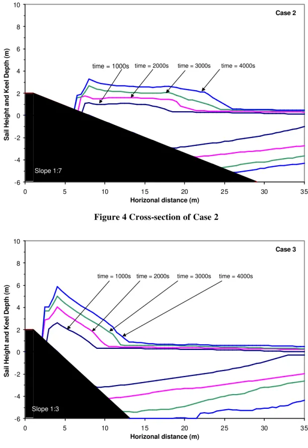
Figures 3 through 6 show the resulting ice pile- ups heights for these four cases. The axis scales are kept the same for each plot for ease of comparison. Each plot shows the ice pile-up that occurred after 1000s, 2000s, 3000s and 4000s. With an ice speed of 0.25m/s, this could represent ice “fetches” of 250m per 1000s, or a total of 1km of incoming ice.

(8)

The value of zero on the vertical axis represents water level. For floating ice, the keel depth to sail height ratio is considered to be 9:1 (in order to maintain neutral buoyancy). The keel depth, however, became limited by water depth in shallow areas.

Case 1 -6 -4 -2 0 2 4 6 8 10 0 5 10 15 20 25 30 35 Horizonal distance (m)

Sail Height and Keel Depth (m)

time = 1000s time = 2000s time = 3000s time = 4000s

Slope 1:14

(9)

Slope 1:7

Figure 4 Cross-section of Case 2

Slope 1:3

(10)

Slope 1:2

Figure 6 Cross-section of Case 4

The pile-up heights after 4000s for each of the four cases were approximately 1.7m, 3.2m, 5.8m and 6.0m, respectively. It can be seen that in these simulations, the ice pile-up heights were greatest for the steeper slopes. It was observed that for the shallower slopes, the ice had a tendency to “back- up” away from the toe of the breakwater, rather than developing any significant increase in height. This may be a result of higher friction due to greater grounding resistance on the relatively long horizontal extent of the pile-up over the gentler slopes.

Additionally, Case 3 was run until a steady-state condition existed. In that case, pile-up height reached a maximum value (Figure 7). Further encroachment of the floating ice sheet merely increased the horizontal extent of the pile- up. This took approximately 12000s (200 minutes), and simulated an extreme case of approximately 3km of ice flowing towards the breakwater. The maximum height reached by the ice was 8.5m, while the grounded ice grew horizontally over 20m from the toe of the breakwater. The maximum force acting in the x-direction at the end of this case was 3.4kN/m.

(11)

Case 3 Extended -6 -4 -2 0 2 4 6 8 10 0 5 10 15 20 25 30 35 Horizonal distance (m)

time = 2000s time = 4000s time = 6000s time = 8000s time = 10000s Slope 1:3 time = 12000s

Figure 7 Ice pile-up for Case 3, leading towards a steady-state condition

The above results are in general agreement with full- scale data found in the literature. For example, Danish observations collected in the Sound linking the Baltic and North Seas found ice pile- up heights exceeding 8m, with an ice thickness of approximately 0.3m (Bruun and Johannesson, 1971). In the “Great Belt” crossing region, also around Denmark, a similar observation was noted, with an ice thickness of 0.35m and pile-up height of 8m (DHI, 1974). In the Beaufort Sea, Kovacs (1983; 1984) observed pile- up heights ranging from 3m to 10.5m for ice thicknesses of 0.25m to 0.5m. Along the northeastern shore of Lake Simcoe, Ontario, Tsang (1974) reported an ice pile-up height of 9m where the ice thickness was about 0.2m. Calculations by Christensen (1994) gave similar results. It can be seen that the numerical model used here does predict these types of observations. We note, though, that field observations usually consist of estimates of pile- up dimensions, shoreline slope, and the oncoming ice thickness. It is difficult to obtain specific measurements of the associated environmental forces, variations in ice cover thickness and properties, or geometry of the area under study (e.g. bathymetry, shoreline geometry, and relevant boundaries). Therefore, we can only use plausible values for the missing information in such observations.

(12)

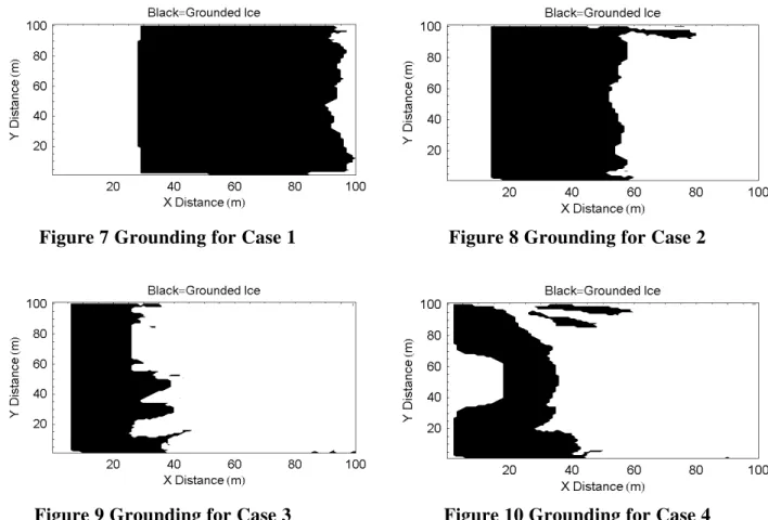
As the ice interacted with the shore, the rubble thickness would increase and often it would “ground” on parts of the shore or seabed. These regions where grounding occurred are shown in Figures 8 through 11 for the four cases. These “grounding plots” represent the grounding that had occurred after 4000s. The initial ice placement of the particles was not perfectly symmetrical, which can be observed in these grounding plots. No attempt was made to start with symmetrically placed particles since the asymmetry appeared to represent an ice sheet more realistically than a uniform cover would in these cases.

Figure 7 Grounding for Case 1 Figure 8 Grounding for Case 2

Figure 9 Grounding for Case 3 Figure 10 Grounding for Case 4

Pressure data was obtained for each case. As an example of this, the resulting pressure distribution for Case 4 is plotted Figure 11.

(13)

Parametric study

Additionally, a small test matrix was designed to examine the influence of ice properties and other parameters on ice pile-up height and grounding. The matrix consisted of four program runs that were built upon the 1:3 breakwater case previously mentioned. Details of the variations in the program runs may be seen in Table 1. Chosen values for the given parameters were based upon conditions that are typical of those observed in the literature (e.g. Tseng, 1974; Kovacs, 1983 and 1984; Christensen, 1994). The results of these four cases after 1000s of ice interaction, as well as those from Case 3 (also after 1000s,) for comparison as a “base case”, are also shown in this table.

Table 1 Parametric study details

Case Ice Thickness (m) Shear Stress (N/m²) Breakwater Slope (vertical: horizontal) f (°) Angle of oncoming ice (°) Ice Pile- up Height (m) 3 0.3 45 1:3 30 270 2.6 5 0.6 45 1:3 30 270 2.9 6 0.3 185 1:3 30 270 4.3 7 0.3 45 1:3 45 270 2.2 8 0.3 45 1:3 30 225 1.9

The pile- up heights, while taken after only 250m of ice had interacted with the breakwater, show expected trends. As expected, increasing either the oncoming ice thickness or the shear stress increased the pile- up height, the latter increasing the pile-up height 1.5 times as high as the base case. Increasing the internal angle of friction slightly decreased the pile-up height, and changing the angle of the advancing ice had the same effect. This is intuitively expected because stronger ice will tend to undergo less deformation and thus produce smaller pile-ups, and changing the angle of the advancing ice (from perpendicular to the breakwater) also reduced pile- up height. Again, these results are in keeping with field observations, such as those observed in Kovacs (1983; 1984).

CONCLUSIONS

This paper presents an overview and the results of a generic study of ice pile-up along shorelines. Numerical simulations of ice pile-up on shorelines were conducted. The numerical model is based on a PIC approach for advecting the ice cover. A depth-averaged approach is employed, where stresses and velocities are averaged over the thickness of the ice cover (or ice pile- up). Rheology is represented by a cohesionless Mohr-Coulomb plastic yield criterion. That model was originally developed to deal with ice forecasting and ice-structure interaction problems. The main modification carried out in the present work is adding grounding forces.

(14)

The numerical results produced the essential features observed in ice pile-up development. For example, when a sufficient length of the ice cover impinges on a shoreline, the pile-up height reaches a maximum value then grows horizontally upstream. Larger pile-ups were found to form on steep slopes. For gentler slopes, pile-up heights were lower. The latter result may be attributed to grounding resistance, which acts over relatively long lengths of the gentler slopes. The larger grounding resistance reduces the force, which produces the pile-up, thereby resulting in smaller pile-up heights.

A parametric study was carried out in order to examine the role of several parameters. Increasing ice strength (i.e. angle of internal friction) reduced pile-up heights. Increasing ice thickness or the driving force was found to increase pile-up heights. The incidence angle of ice movement against the shoreline was also examined. Changing the direction from perpendicular to the shoreline reduced pile- up heights. The numerical results were also in general agreement with published field observations.

The present numerical simulations proved capable of quantifying the impact of various variables on the resulting ice pile- up behaviour. Such a numerical approach can greatly reduce uncertainties that have been encountered in the design of coastal structures that are subjected to ice encroachment. Further, these models can help to identify potential problems of ice interacting with coastal structures. These models can aid researchers during investigations of ice-structure interaction scenarios by helping to “narrow down” critical situations, which can then cut-down the amount of physical modelling needed, saving costs and time. This type of numerical model can be a powerful tool for future coastal engineering design.

ACKNOWLEDGEMENT

The support of the Program on Energy Research and Development (PERD) is gratefully acknowledged.

REFERENCES

Beltaos, S., editor, (1995). "River Ice Jams," Water Resources Publications, Highlands Ranch, Colorado, U.S., 372 p.

Bruun, P.(editor) and Johannesson, P. (1971). The interaction between ice and coastal structures. Proceedings POAC’71. Vol.1, pp. 683-712. Trondheim, Norway.

Christensen, F.T. (1994). Ice Ride-up and Pile- up on Shores and Coastal Structures. Journal of Coastal Research, Vol.10, No.3, pp.681-701.

(15)

Danish Hydraulic Institute. (1974). “Hydraulic Investigations for Saltholm Airport. Report no.2, Preliminary ice report.” (Translation). Report by Danish Hydraulic Institute for Projektorganisation Saltholm,. Copenhagen, Denmark.

Kovacs, A. (1983). Sea Ice on the Norton Sound and Adjacent Bering Sea Coasts. Proceedings POAC’83, Vol. 4, pp 654-666. Espoo, Finland.

Kovacs, A. (1983). “Shore Ice Ride-Up and Pile-Up Features, Part I: Alaska’s Beaufort Sea Coast.” CRREL Report 83-9, U.S. Army Cold Regions Research and Engineering Laboratory, Hanover, New Hampshire, U.S.A.

Kovacs, A. (1984). “Shore Ice Ride-Up and Pile-Up Features, Part I: Alaska’s Beaufort Sea Coast – 1983 and 1984.” CRREL Report 84-26, U.S. Army Cold Regions Research and Engineering Laboratory, Hanover, New Hampshire, U.S.A.

Sayed, M. (1998). “Ice model development: implementation,” Technical Report HYD-TR-036, Canadian Hydraulics Centre, National Research Council, Ottawa, Ontario, Canada, June 1998.

Sayed, M., and Carrieres, T. (1999). Overview of a new operational ice forecasting model,

ISOPE ’99. Vol. II, pp.622-627. Brest, France.

Sayed, M., Frederking, R. and Barker, A. (2000) Numerical Simulation of Pack Ice Forces on Structures: a Parametric Study. ISOPE ’00. Vol.1, pp.656-662. Seattle, U.S.A

Timco, G.W., Willis, D.H. and Wright, B.D. 1995. Ice Action on Armour Rocks with Application to an Artificial Island Concept. Proceedings of the Second International Conference on the Development of the Russian Arctic Offshore, RAO’95, pp 284- 290, St. Petersburg, Russia.

Tseng, G. (1974). Ice Piling on Lakeshores. CCIW Scientific Series Report No. 35, Burlington, Ont., Canada