Characterizing 51 Eri b from 1 to 5 μm: a partly cloudy exoplanet

Publisher’s version / Version de l'éditeur:

The Astronomical Journal, 154, 1, 2017-06-16

READ THESE TERMS AND CONDITIONS CAREFULLY BEFORE USING THIS WEBSITE. https://nrc-publications.canada.ca/eng/copyright

Vous avez des questions? Nous pouvons vous aider. Pour communiquer directement avec un auteur, consultez la

première page de la revue dans laquelle son article a été publié afin de trouver ses coordonnées. Si vous n’arrivez pas à les repérer, communiquez avec nous à PublicationsArchive-ArchivesPublications@nrc-cnrc.gc.ca.

Questions? Contact the NRC Publications Archive team at

PublicationsArchive-ArchivesPublications@nrc-cnrc.gc.ca. If you wish to email the authors directly, please see the first page of the publication for their contact information.

NRC Publications Archive

Archives des publications du CNRC

This publication could be one of several versions: author’s original, accepted manuscript or the publisher’s version. / La version de cette publication peut être l’une des suivantes : la version prépublication de l’auteur, la version acceptée du manuscrit ou la version de l’éditeur.

For the publisher’s version, please access the DOI link below./ Pour consulter la version de l’éditeur, utilisez le lien DOI ci-dessous.

https://doi.org/10.3847/1538-3881/aa74db

Access and use of this website and the material on it are subject to the Terms and Conditions set forth at

Characterizing 51 Eri b from 1 to 5 μm: a partly cloudy exoplanet

Rajan, Abhijith; Rameau, Julien; Rosa, Robert J. De; Marley, Mark S.;

Graham, James R.; Macintosh, Bruce; Marois, Christian; Morley, Caroline;

Patience, Jennifer; Pueyo, Laurent; Saumon, Didier; Ward-duong, Kimberly;

Ammons, S. Mark; Arriaga, Pauline; Bailey, Vanessa P.; Barman, Travis;

Bulger, Joanna; Burrows, Adam S.; Chilcote, Jeffrey; Cotten, Tara; Czekala,

Ian; Doyon, Rene; Duchêne, Gaspard; Esposito, Thomas M.; Fitzgerald,

Michael P.; Follette, Katherine B.; Fortney, Jonathan J.; Goodsell, Stephen

J.; Greenbaum, Alexandra Z.; Hibon, Pascale; Hung, Li-wei; Ingraham,

Patrick; Johnson-groh, Mara; Kalas, Paul; Konopacky, Quinn; Lafrenière,

https://publications-cnrc.canada.ca/fra/droits

L’accès à ce site Web et l’utilisation de son contenu sont assujettis aux conditions présentées dans le site LISEZ CES CONDITIONS ATTENTIVEMENT AVANT D’UTILISER CE SITE WEB.

NRC Publications Record / Notice d'Archives des publications de CNRC:

https://nrc-publications.canada.ca/eng/view/object/?id=bc2d9898-8a62-4fe0-b6e4-b1cf7949d2b4 https://publications-cnrc.canada.ca/fra/voir/objet/?id=bc2d9898-8a62-4fe0-b6e4-b1cf7949d2b4

Characterizing 51 Eri b from 1 to 5

μm: A Partly Cloudy Exoplanet

Abhijith Rajan1, Julien Rameau2, Robert J. De Rosa3, Mark S. Marley4, James R. Graham3, Bruce Macintosh5, Christian Marois6,7, Caroline Morley8, Jennifer Patience1, Laurent Pueyo9, Didier Saumon10, Kimberly Ward-Duong1, S. Mark Ammons11, Pauline Arriaga12, Vanessa P. Bailey5, Travis Barman13, Joanna Bulger14, Adam S. Burrows15, Jeffrey Chilcote16, Tara Cotten17,

Ian Czekala5, Rene Doyon2, Gaspard Duchêne3,18, Thomas M. Esposito3, Michael P. Fitzgerald12, Katherine B. Follette5, Jonathan J. Fortney19, Stephen J. Goodsell20, Alexandra Z. Greenbaum21, Pascale Hibon22, Li-Wei Hung12, Patrick Ingraham23, Mara Johnson-Groh7, Paul Kalas3,24, Quinn Konopacky25, David Lafrenière2, James E. Larkin12, Jérôme Maire25, Franck Marchis24,

Stanimir Metchev26,27, Maxwell A. Millar-Blanchaer28,35, Katie M. Morzinski29, Eric L. Nielsen5,24, Rebecca Oppenheimer30, David Palmer11, Rahul I. Patel31, Marshall Perrin9, Lisa Poyneer11, Fredrik T. Rantakyrö22, Jean-Baptiste Ruffio5, Dmitry Savransky32, Adam C. Schneider1, Anand Sivaramakrishnan9, Inseok Song17, Rémi Soummer9, Sandrine Thomas23,

Gautam Vasisht28, J. Kent Wallace28, Jason J. Wang3, Sloane Wiktorowicz33, and Schuyler Wolff34 1_{School of Earth and Space Exploration, Arizona State University,}

P.O. Box 871404, Tempe, AZ 85287, USA;arajan6@asu.edu

2_{Institut de Recherche sur les Exoplanètes, Départment de Physique,}

Université de Montréal, Montréal QC H3C 3J7, Canada

3_{Astronomy Department, University of California, Berkeley; Berkeley CA 94720, USA} 4_{NASA Ames Research Center, Mountain View, CA 94035, USA}

5_{Kavli Institute for Particle Astrophysics and Cosmology, Stanford University, Stanford, CA 94305, USA} 6_{National Research Council of Canada Herzberg, 5071 West Saanich Rd, Victoria, BC V9E 2E7, Canada}

7_{University of Victoria, 3800 Finnerty Rd, Victoria, BC V8P 5C2, Canada} 8_{Department of Astronomy, Harvard University, Cambridge, MA 02138, USA}

9_{Space Telescope Science Institute, Baltimore, MD 21218, USA}

10_{Los Alamos National Laboratory, P.O. Box 1663, MS F663, Los Alamos, NM 87545, USA} 11_{Lawrence Livermore National Laboratory, Livermore, CA 94551, USA}

12_{Department of Physics & Astronomy, University of California, Los Angeles, CA 90095, USA} 13_{Lunar and Planetary Laboratory, University of Arizona, Tucson AZ 85721, USA}

14_{Subaru Telescope, NAOJ, 650 North A’ohoku Place, Hilo, HI 96720, USA} 15_{Department of Astrophysical Sciences, Princeton University, Princeton, NJ 08544, USA} 16_{Dunlap Institute for Astronomy & Astrophysics, University of Toronto, Toronto, ON M5S 3H4, Canada}

17_{Department of Physics and Astronomy, University of Georgia, Athens, GA 30602, USA} 18

Univ. Grenoble Alpes/CNRS, IPAG, F-38000 Grenoble, France

19_{Department of Astronomy, UC Santa Cruz, 1156 High Street, Santa Cruz, CA 95064, USA} 20

Gemini Observatory, 670 N. A’ohoku Place, Hilo, HI 96720, USA

21_{Department of Astronomy, University of Michigan, Ann Arbor MI 48109, USA} 22_{Gemini Observatory, Casilla 603, La Serena, Chile}

23_{Large Synoptic Survey Telescope, 950N Cherry Av, Tucson, AZ 85719, USA} 24_{SETI Institute, Carl Sagan Center, 189 Bernardo Avenue, Mountain View, CA 94043, USA} 25_{Center for Astrophysics and Space Science, University of California San Diego, La Jolla, CA 92093, USA}

26_{Department of Physics and Astronomy, Centre for Planetary Science and Exploration,}

The University of Western Ontario, London, ON N6A 3K7, Canada

27_{Department of Physics and Astronomy, Stony Brook University, Stony Brook, NY 11794-3800, USA} 28_{Jet Propulsion Laboratory, California Institute of Technology, Pasadena, CA 91125, USA}

29_{Steward Observatory, University of Arizona, Tucson AZ 85721, USA}

30_{Department of Astrophysics, American Museum of Natural History, New York, NY 10024, USA} 31_{Infrared Processing and Analysis Center, California Institute of Technology, Pasadena, CA 91125, USA}

32_{Sibley School of Mechanical and Aerospace Engineering, Cornell University, Ithaca, NY 14853, USA} 33_{The Aerospace Corporation, El Segundo, CA 90245, USA}

34_{Department of Physics and Astronomy, Johns Hopkins University, Baltimore, MD 21218, USA} Received 2017 March 24; revised 2017 May 8; accepted 2017 May 8; published 2017 June 16

Abstract

We present spectrophotometry spanning 1–5 μmof 51 Eridani b, a 2–10MJup planet discovered by the Gemini

Planet Imager Exoplanet Survey. In this study, we present new K1 (1.90–2.19 μm) and K2 (2.10–2.40 μm) spectra taken with the Gemini Planet Imager as well as an updated LP(3.76 μm) and new MS(4.67 μm) photometry from

the NIRC2 Narrow camera. The new data were combined with J(1.13–1.35 μm) and H(1.50–1.80 μm) spectra from the discovery epoch with the goal of better characterizing the planet properties. The 51Erib photometry is redder than field brown dwarfs as well as known young T-dwarfs with similar spectral type (between T4 and T8), and we propose that 51 Eri b might be in the process of undergoing the transition from L-type to T-type. We used two complementary atmosphere model grids including either deep iron/silicate clouds or sulfide/salt clouds in the photosphere, spanning a range of cloud properties, including fully cloudy, cloud-free, and patchy/intermediate-opacity clouds. The model fits suggest that 51Erib has an effective temperature ranging between 605 and 737 K, a solar metallicity, and a surface gravity of log(g) = 3.5–4.0 dex, and the atmosphere requires a patchy cloud atmosphere to model the spectral energy distribution (SED). From the model atmospheres, we infer a luminosity

https://doi.org/10.3847/1538-3881/aa74db

© 2017. The American Astronomical Society. All rights reserved.

for the planet of −5.83 to −5.93 (logL L), leaving 51Erib in the unique position of being one of the only

directly imaged planets consistent with having formed via a cold-start scenario. Comparisons of the planet SED against warm-start models indicate that the planet luminosity is best reproduced by a planet formed via core accretion with a core mass between 15 and 127 MÅ.

Key words:instrumentation: adaptive optics – planets and satellites: atmospheres – planets and satellites:

composition – planets and satellites: gaseous planets – stars: individual (51 Eridani)

Supporting material:data behind figures

1. Introduction

Until recently, most of the imaged planetary-mass companions detected were typically orbiting their parent star at large orbital separations, >30au. However, new instrumentation with second-generation adaptive optics such as the Gemini Planet Imager (GPI; Macintosh et al. 2014) and Spectro-Polarimetric High-contrast Exoplanet REsearch (SPHERE; Beuzit et al.2008) are now routinely obtaining deep contrasts ( 10 10_> 5_– 6_{)in the inner}

arcsecond (5–30 au). The recent detection of new companions (Macintosh et al. 2015; Konopacky et al. 2016; Wagner et al. 2016; Milli et al. 2017) and debris disks (Currie et al. 2015; Millar-Blanchaer et al. 2016; Wahhaj et al. 2016; Bonnefoy et al. 2017) showcase the advances made by these next-generation Adaptive Optics (AO) systems. Direct imaging, unlike nondirect methods such as radial velocity and transits, measures light from companions directly, which permits measuring the atmospheric spectrum, with the caveat that the final calibration is dependent on a complete understanding of the stellar properties. These new AO instruments combine excellent image stability and high throughput with Integral Field Unit (IFU) spectrographs, enabling the measurement of a spectrum of the planet in the near-infrared (IR) wavelength range. Combining the near-IR spectra with mid-IR photometry from instruments such as Keck/NIRC2, MagAO/Clio, or LBT/LMIRCam provides valuable constraints on the effective temperature and nonequilibrium chemistry when undertaking comprehensive modeling of the exoplanet spectral energy distribution (SED).

In this study we focus on the planetary companion 51Eridanib (51 Eri b; Macintosh et al. 2015). 51Erib is the first planet discovered by the Gemini Planet Imager Exoplanet Survey (GPIES), a survey targeting 600 young and nearby stars using GPI to search for exoplanets. The planet orbits 51EriA, a young F0IV star that is part of the βPic moving group (Zuckerman et al. 2001). In this study, we adopt an age of 26±3Myr for the βPic moving group (Nielsen et al.2016). However, the age of the group is a topic of considerable debate and has been revised several times, for example, 21±4 (Binks & Jeffries 2014), 23±3 (Mamajek & Bell 2014), 20±6 (Macintosh et al. 2015), and 24±3 (Bell et al. 2015). The primary is part of a hierarchical triple with two M-star companions, GJ3305AB, separated from the primary by ∼2000au (Feigelson et al. 2006; Kasper et al. 2007; Montet et al. 2015). 51EriA is known to have an IR excess, and a debris disk was detected in the Herschel Space Observatory 70 and 100 μmbands with a very low IR luminosity of

LIR/L= ´2 10-6 and a lower limit on the inner radius of

82au (Riviere-Marichalar et al.2014), as well as a detection at 24 μmwith the Spitzer Space Telescope (Rebull et al. 2008). The debris disk was not detected in Macintosh et al. (2015), which, given the low fractional luminosity, would be extremely challenging. The analysis of the atmosphere of 51Erib by

Macintosh et al. (2015) was based on GPI JH spectra

(1.1–1.8 μm) and Keck LP photometry (3.76 μm), using two

different model atmosphere grids to estimate the planet properties. While the models agreed on the temperature and luminosity, they were highly discrepant in terms of best fitting the surface gravity with one grid, suggesting low surface gravity and youth, while the other required a high surface gravity and an old planet. Similarly, one grid best fit the atmosphere when using a linear combination of cloudy and clear models, while the other best fit the data with a clear atmosphere. These discrepancies indicate that more data are required to fully constrain the planet parameters.

In this paper, we present new observations and a revised data analysis that can be used to discriminate between some of the disagreements. In Section 2, we present the first K1 (1.90–2.19 μm) and K2 (2.10–2.40 μm) spectra of the planet taken with GPI. We also present updated LPphotometry and

new observations of the planet in the MSband (4.67 μm). In

Section3, we present new near-IR photometry of the star and revise the stellar SED used in the rest of the analysis. In Section 4, we examine the near- and mid-IR photometry of 51Erib in relation to that of other field and young brown dwarfs through the brown dwarf color–magnitude diagram (CMD). We also compare the near-IR spectrum of 51Erib to field brown dwarfs and planetary-mass companions to estimate the best-fitting spectral type of the planet. Finally, in Section 5 we model the planet SED using two different grids spanning effective temperatures from 450 to 1000 K with deep iron/silicate clouds or sulfide/salt clouds. The 1–5μmSED in combination with these two model grids will help refine the planet properties and clarify whether the atmosphere is best fit by clouds or not.

2. Observations and Data Reduction

2.1. GPI K1 and K2

51Erib was observed with the Integral Field Spectrograph (IFS) of GPI through the K1 filter on 2015 November 06 UT and 2016 January 28 and through the K2 filter on 2015 December 18 UT (see Table1). Standard procedures, namely using an argon arc lamp, were used to correct the data for instrumental flexure. To maximize the parallactic rotation for angular differential imaging (ADI; Marois et al.2006), the observations were centered on the meridian passage. All of the GPI data sets underwent the same initial data processing steps using the GPI Data Reduction Pipeline v1.3.0 (DRP; Perrin et al. 2014). The processing steps included dark-current subtraction and bad-pixel identification and interpolation; this is followed by compensating for instrument flexure using the argon arc spectrum (Wolff et al. 2014). Following this step, the microspectra are extracted to generate the IFS data cubes (Maire et al. 2014). During the process of generating the 3D (x, y, λ) cubes, the microspectra data are resampled tol dl =65and 75 at K1 and K2, respectively, after which they are interpolated to a common wavelength scale and

corrected for geometric distortion (Konopacky et al. 2014). The data cubes are then aligned to a common center calculated using the four satellite spots (Wang et al.2014). The satellite spots are copies of the occulted central star, generated by the use of a regular square grid printed on the apodizer in the pupil plane (Marois et al. 2006; Sivaramakrishnan & Oppenheimer 2006; Macintosh et al.2014). The satellite spots also help convert the photometry from contrast units to flux units. No background subtraction was performed since the following steps of high-pass filtering and point-spread function (PSF) subtraction efficiently remove this low-frequency component.

Further steps to remove quasi-static speckles and large-scale structures were executed outside the DRP. Each data cube was filtered using an unsharp mask with a box width of 11 pixels. The four satellite spots were then extracted from each wavelength slice and averaged over time to obtain templates of the star PSF. The Linear Optimized Combination of Images algorithm (LOCI; Lafrenière et al.2007)was used to suppress the speckle field in each frame using a combination of

aggressive parameters: dr = 5 px, NA = 200 PSF FWHM,

g = 0.5, and Nd=0.5 0.75– FWHM for the three data sets, where dr is the radial width of the optimization zone, NAis the

number of PSF FWHM that can be included in the zone, g is the ratio of the azimuthal and radial widths of the optimization zone, and Nδ defines the maximum separation of a potential astrophysical source in FWHM between the target and the reference PSF. The residual image of each wavelength slice was built from a trimmed (10%) temporal average of the sequence.

Final K1 and K2 broadband images were created using a weighted mean of the residual wavelength frames according to the spectrum of the planet, examples of which can be found in Figure 1. These broadband images were used to extract the astrometry of the planet in each data set thanks to a higher signal-to-noise ratio (S/N) than in individual frames. To do so, a negative template PSF was injected into the raw data at the estimated position and flux of the planet before applying LOCI and reduced using the same matrix coefficients as the original reduction (Marois et al. 2010). The process was iterated over these three parameters (x position, y position, flux) with the amoeba simplex optimization (Nelder & Mead1965)until the integration squared pixel noise in a wedge of 2×2 FWHM was minimized. The best-fit position was then used to extract

the contrast of the planet in each data set. The same procedure was executed in the noncollapsed wavelength residual images, varying only the flux of the negative template PSF and keeping the position fixed to prevent the algorithm from catching nearby brighter residual speckles in the lower S/N spectral slices. To measure uncertainties, we injected the template PSF with the measured planet contrast into each data cube at the same separation and 20 different position angles. We measured the fake signal with the same extraction procedure. The contrasts measured in the 2015 November 06 and 2016 January 28 K1 data sets agreed within the uncertainties, the latter having significantly better S/N, and were combined with the weighted mean to provide the final planet contrasts.

Table 1 Observations of 51Erib

Date Instrument Filter Total Int. Field Averaged Averaged Averaged

time (minutes) Rot. (°) air mass DIMM seeing (as) MASSt (ms)0

2015 Jan 30 GS/GPI Ja 70 23.8 1.15 0.52 3.26 2014 Dec 18 GS/GPI Ha 38 37.7 1.14 L L 2015 Nov 06 GS/GPI K1b 55 30.5 1.17 0.38 1.56 2015 Dec 18 GS/GPI K2b _{103 71.7 1.22 0.69 0.94} 2016 Jan 28 GS/GPI K1b 97 55.5 1.15 0.86 4.40 2015 Oct 27 Keck/NIRC2 LPb 100 74.2 1.10 L L 2016 Jan 02 Keck/NIRC2 MSb 139 115.7 1.18 L L 2016 Jan 21 Keck/NIRC2 MSb 174 116.0 1.21 L L 2016 Feb 04 Keck/NIRC2 MSb 148 101.4 1.21 L L 2016 Feb 05 Keck/NIRC2 MSb 142 102.1 1.21 L L Notes. a_{Macintosh et al. (2015).} b_{This work.}

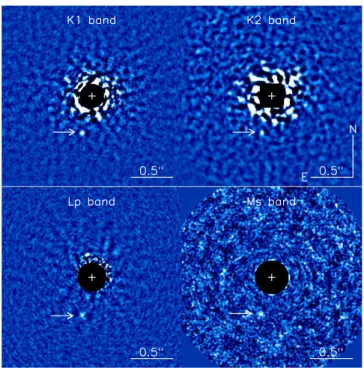
Figure 1.Final PSF-subtracted images of 51Erib. Top: LOCI-reduced GPIES images at the K1 (2016 January 28, left) and K2 bands (2015 December 18, right). Bottom: pyKLIP-reduced NIRC2 images, smoothed with a box of width 2 pixels, at LP(2015 October 27, left), and a combined image of all four

MSdata sets (right). The images are scaled linearly, but are different in each

2.1.1. Spectral Covariances

The estimation of a directly imaged planet’s properties from its measured spectrum is complicated by the fact that spectral covariances are present within the extracted spectra. In the GPI data, these are caused by the residual speckle noise in the final PSF-subtracted image and the oversampling of the individual microspectra during the initial data reduction process. Atmos-phere modeling without properly accounting for these covar-iances can lead to biased results. We present the derivation of the correlation using the parameterization of Greco & Brandt (2016)in theAppendix.

We use the spectral covariance when carrying out a comparison of the planet spectrophotometry against other field and young dwarfs as well as during model fitting. The covariance helps correctly account for the correlation in the spectra while also increasing the importance of the photometry, and thus the use of the covariance tends to move the best fits toward cooler temperatures when compared to using the variance directly.

2.2. Keck LP

We observed the 51Eri system on 2015 October 27 in the LP

filter with the NIRC2 camera (McLean & Sprayberry2003)at the Keck II observatory (Program ID U055N2). The observa-tions were taken in ADI mode, starting ∼1hr prior to meridian crossing to maximize the field-of-view rotation. The target was observed for ∼3hr total, with 100minutes of on-source integration. The observations were acquired using the 400 mas focal plane mask and the circular undersized “in-circle” cold stop. To calibrate the planet brightness, unsaturated observa-tions of the star were taken at the end of the observing sequence. The images were dark and flat-field corrected. We used the KS-band lamp flats to build the flat-field and masked

hot and bad pixels. As these observations were taken after the 2015 April servicing of NIRC2, the geometric distortion was corrected using the solution presented in Service et al. (2016, updating the original Yelda et al. 2010 solution), with an updated plate scale of 9.971±0.004 mas pixel−1 and the offset angle β (0.262 ± 0.020) that is required when calculating the position angle prior to rotating the images to put north up (Yelda et al.2010). Postprocessing of the data was carried out using the Python version of the Karhunen–Loève (KL) Image Projection algorithm (KLIP; Amara & Quanz2012; Soummer et al.2012), pyKLIP (Wang et al.2015). As part of this study, we included an NIRC2 module in the pyKLIP code base that is publicly available for users.36The algorithm accepts aligned images and performs PSF subtraction using KLIP where the image can be divided into sections both radially and azimuthally. Aside from the choice of zones, two main parameters were adjusted, the number of modes used in the KL transform and an exclusion criterion for reference PSFs, similar to Nδ mentioned above, that determine the number of pixels an astrophysical source would move due to the rotation of the reference stack. We carried out a parameter search where the four parameters mentioned were varied to optimize the S/N in the planet signal. The planet photometry was estimated using the method described above for the K1 and K2 filters, using a negative template PSF. The LPmagnitude contrast for the star/

planet is 11.58±0.15 mag, which agrees very well with the

photometry in the original epoch, 11.62±0.17 mag. The weighted mean of both measurements is used in the rest of the analysis.

2.3. Keck MS

Observations of 51Erib were taken in the MS-band filter

over four separate half nights on 2016 January 02 and 21 and 2016 February 04 and 05 with the Keck/NIRC2 Narrow camera. The details of the observations are presented in Table1. Each night the target was observed for a period of ∼6 hr, as part of two separate NASA and UC Keck observing programs (Program IDs N179N2, U117N2). The data were obtained in ADI mode, with the field of view rotating at the sidereal rate. To reduce the effects of persistence and enable accurate thermal background correction, the star was nodded across the detector in four large dithers centered in each quadrant of the detector. Furthermore, to prevent saturation of the detector by the thermal background, the exposures were limited to 0.3 s with 200 coadds, without using an occulting spot. The images were dark and flat-field corrected with twilight sky flats, followed by hot and bad pixel correction. As with the LPdata, the solution provided by Service et al. (2016)

was used to correct the NIRC2 Narrow camera geometric distortion. Finally, all of the images were rotated to put north up.

An additional step required for the MS-band data that is not

as critical for the other data sets is the background subtraction. Since the thermal background at 5 μmis large and highly time variable, rather than median combine or high-pass filter to remove the background, we adopted the least-squares sky-subtraction algorithm proposed in Galicher et al. (2011). For each point in the dither pattern, the algorithm uses the images where the star is in one of the other three positions to construct a reference library. We used a ring centered on the star to estimate the thermal background in each image, with an inner annulus of 24 pixels and an outer annulus of 240 pixels. The final calibration step involved aligning the background-corrected PSFs. Since the core of the PSF is saturated in the data, we aligned the data using two different methods: (1) fitting a 2D Gaussian to the wings of the stellar PSF to estimate the center of the star and then shifting the PSF to a predetermined pixel value to align all the images and (2) using the rotation symmetry of the PSF using the method described in Morzinski et al. (2015). To compare the two methods, we calculated the residuals between images aligned using the methods and compared the noise in the residuals and found them to be similar, so we chose to go with the 2D Gaussian, which is computationally faster.

The procedure used for the PSF subtraction for the MSdata

was similar to that for the LPdata. The planet is not detected in

each of the individual half-night data sets, requiring a combination of all four half nights to increase the S/N to detect the planet flux. To correctly combine the planet flux across the multiple epochs, we adjusted the PA to account for the astrophysical motion of the planet around the star, for which we used the best-fitting orbit presented in De Rosa et al. (2015). In the month between the first and last data sets, the planet rotated ∼0°.48 or ∼0.4pixel, which is a sufficiently large correction that it must be included in the data reduction. Each night’s data were reduced individually to generate 603 PSF-subtracted images. These images were then combined by dividing each image into 13 annuli, which were combined 36_{https://bitbucket.org/pyKLIP/pyklip}

using a weighted mean, where the weights are the inverse variance in each annulus. As seen in Figure 1, we detect the planet signal at ∼2–3σ. To confirm that we are detecting the planet, we rotated the data to match the PA value of the LP

epoch to find that the flux peak in the MS band matches the

location of the planet in LP. We measured a star-to-planet

contrast of 11.5 mag using the same procedure as described for the LP data. We injected 25 fake PSFs that were scaled to

match the contrast measured for the planet and detected the fakes at the same contrast as the planet. The final magnitude of the star-to-planet contrast in the MSis 11.5±0.5 mag.

3. Results

To estimate the stellar parameters of 51EriA, Macintosh

et al. (2015) made use of Two Micron All-Sky Survey

photometry (2MASS; Cutri et al.2003; Skrutskie et al.2006). However, the J- and H-band photometry for the star are flagged as “E,” indicating that the photometry is of the poorest quality and potentially unreliable (as compared to an “A” flag for the the K-band photometry). Further, the study used photometry taken with the Wide-field Infrared Survey Explorer (WISE; Wright et al. 2010) in the W1 filter (l = 3.35μm,eff

1.11

l

D = μm) as an approximation for the LP-band

magni-tude of the primary star. The photometry for 51EriA in W1, from the AllWISE catalog (Cutri et al.2013), has large errors and contributes to more than half the error budget of the final planet photometry. In this study, we thus chose to reobserve the star in the JHKSfilters and fit all the available photometry to

estimate the photometry in filters where no calibrated stellar data exist.

3.1. Revised Stellar Photometry at J, H, and KS

The 2MASS near-IR colors of 51EriA were compared to empirical colors for young F0 stars taken from Kenyon & Hartmann (1995), where an F0IV star should have J−H=0.13 mag and H−K=0.03 mag. The colors of 51EriA estimated using the 2MASS photometry are however discrepant, with

J−H=−0.03±0.08 and H−K=0.23±0.08 mag. The

discrepant near-IR colors combined with poor-quality flags suggest that the published photometry is potentially incorrect.

We observed the star 51EriA using the 6.5m MMT on Mt. Hopkins with the ARIES instrument (McCarthy et al.1998)on 2016 February 28 UT under photometric conditions. We obtained data in the MKO JHKSbroadband filters (Tokunaga

et al. 2002), for a total of 3.4 minutes in each filter. To flux calibrate these observations, we observed a photometric standard star at a similar air mass as 51EriA, HR1552 (Carter1990). The raw images for both targets were processed through a standard near-IR reduction pipeline, performing dark-current subtraction, flat-field calibration, and bad-pixel correction. Aperture photometry was performed on both targets, with the curve of growth used to select an aperture that minimized the error on the measured flux. The measured brightness of 51EriA is presented in Table2.

Converting the MKO KS-band measurement into the 2MASS

system using empirical relations37 _{yields K}

4.551

S,2MASS= 

0.032 mag, which is within 1σ of the published 2MASS

photometry. Furthermore, the J−H and H−K colors estimated from the revised photometry are 0.128±

0.037mag and 0.016±0.039mag, which are consistent with the empirical expectations.

The published 51Erib spectrum in Macintosh et al. (2015) was calibrated using the Pickles stellar models (Pickles1998) to estimate the spectrum of the primary, where each band was scaled using the published 2MASS photometry. In Figure2we present a comparison between the published spectrum and one scaled using the new MKO photometry, using the same stellar models. The revised photometry scales the planet spectrum higher by ∼10% in the J band and ∼15% in the H band, which is significant given the high S/N of the H-band data.

3.2. Fitting the SED of 51EriA

To mitigate the effects of incorrect photometry, rather than scale the spectrum in pieces using the relevant broadband

Table 2 System Properties

Property 51_EriA 51_Erib

Distance (pc) L 29.43±0.29a

Age (Myr) L 26±3b

Spectral Type F0IV T6.5_±1.5

L L log( ) 0.85-+0.070.06c -5.83-+0.120.15to 5.93- -+0.140.19d Teff 7331±30Ke 605–737Kd g log 3.95±0.04e _3.5–4.0d JMKO 4.690±0.020d 19.04±0.40d,f HMKO 4.562±0.031d _{18.99±0.21}d KS MKO, 4.546±0.024d 18.49±0.19d KMKO 4.600±0.024e 18.67±0.19d LP 4.604±0.014e 16.20±0.11d,g MS 4.602±0.014e 16.1±0.5d Notes. a

Hipparcoscatalog (van Leeuwen2007).

b_{Nielsen et al. (2016).} c_{Macintosh et al. (2015}

)using hot-start predictions.

d_{This work.}

e_{Stellar photometry estimated using SED fit.} f_{Distance modulus = 2.34}

±0.02mag.

g_{Weighted mean of the two L}

Pobservations.

Figure 2.Comparison of the JH spectra of 51Erib using the literature 2MASS values against the new photometry measured in this study. The updated photometry increases the planet flux by ∼10% in J and ∼15% in the H band. The updated stellar photometry is used in the remainder of this study. However, the final stellar spectrum used to correct the planet spectrum does not depend on individual filter photometry, as in Macintosh et al. (2015)and shown in this plot, but is generated by modeling the full stellar SED prior to converting the planet spectra from contrast to flux units.

photometry, we decided to fit the full SED of 51EriA using literature photometry and colors, including Geneva U B B, 1, ,

B2,V V G1, , (Rufener & Nicolet 1988), Tycho2 B VT, T/

Hipparcos HP(ESA1997; Høg et al.2000), MKO JHKS(this

work), and WISE W1,W2 (Cutri et al.2013)measurements. We made use of the Geneva color relations as constraints to the full SED fit since the published Geneva V magnitude, which anchors the colors to estimate the remaining photometry, appears to be offset by ∼5% when compared to the Tycho2 photometry. The

WISE W2 photometry was corrected using the Cotten & Song

(2016)relation for bright stars. We combine the photometry with model stellar atmospheres from the BT-NextGen grid38_(Allard et al.2012), and we estimated the stellar spectrum using a five-parameterMarkov chain Monte Carlo (MCMC) grid search. The

best-fit atmosphere was found with Teff=733130 K,

g

log =3.950.04, M H[ ]= -0.120.06, and a stellar radius R =1.450.02 R (assuming a parallax of 33.98 ±

0.34 mas; van Leeuwen 2007). No correction for extinction is performed as the extinction in the direction of 51Eri is negligible (AV =0.00; Guarinos 1992). These values are consistent with previous literature estimates (e.g., Koleva &

Vazdekis 2012). The final SED of 51EriA is shown in

Figure 3, which highlights the significantly discrepant 2MASS

JH-band photometry that was used previously to calibrate the

spectrum of 51Erib. We extracted MKO K and NIRC2 LPand

MS photometry from the SED fit using the filter response

functions presented in Tokunaga et al. (2002); see Table2. 3.2.1. Confirming the Stellar LPPhotometry

51Erib emits a substantial amount of flux in the mid-IR, and LP photometry in Macintosh et al. (2015) was used to

constrain the effective temperature of the planet. There exists no LP flux measurement for the star, so they used the W1

magnitude reported in the AllWISE catalog (W1 =4.543 0.210;Cutri et al.2013)and assumed a color of W1 -LP =0

based on the F0IV spectral type of 51Eri (Abt & Morrell1995). The LPphotometry we estimated via the SED fits for 51Eri is

LP= 4.604±0.014 mag, which is consistent with the value

reported in Macintosh et al. (2015, 4.52 ± 0.21 mag) but with significantly smaller uncertainties.

As a final check for consistency, the 2MASS KSmagnitude

of 51Eri (KS,2MASS=4.5370.024) was used instead as a starting point. The KS-LPcolor for early F-type dwarfs and

subgiants was estimated by folding model stellar spectra (7200Teff K7400, 4.0logg4.5, [M H]=0) from the BT-SETTL model grid through the relative spectral response of the 2MASS KS(Cohen et al.2003)and NIRC2 LP

filters. Over this range of temperatures and surface gravities, the color was calculated as KS-LP= -0.0010.001. In order to realistically assess the uncertainties on this color, the near- to thermal-IR spectra of F-type dwarfs and subgiants within the IRTF library (Rayner et al.2009)were processed in the same fashion, resulting in a KS-LP=0.0140.055. A color of KS -LP= -0.0010.055 was adopted based on the color calculated from the model grid and the uncertainty calculated from the empirical IRTF spectra. This color, combined with the KS,2MASSmagnitude of 51Eri, gives an LP

apparent magnitude of 4.538±0.060. The estimates for the stellar LPmagnitude are within 1σ of each other, so we adopt

the value derived from the SED fit: LP=4.604±0.014 mag.

3.3. 51Erib SED

We present the final SED of the planet 51Erib in Figure4

and use it to analyze the system properties in the following sections. Using the stellar SED estimated earlier, we have updated the J and H spectra that were published in Macintosh et al. (2015). In Table 2, we present the properties of the

system, including updated MKO JHK and NIRC2 L MP S

photometry for both the star and the planet. A future study will refine the orbital solution presented in De Rosa et al. (2015).

4. Analysis

4.1. Comparison against Field Brown Dwarfs

We plot a series of CMDs for ultracool objects in Figure5and compare the photometry of field M, L, and T dwarfs and young

Figure 3.Top panel: photometry of 51EriA from the literature, and from the results presented in this study (solid symbols). One hundred models were randomly selected from the MCMC search and are plotted (translucent black curves). For each model, the synthetic magnitude was calculated for each filter. The median value for each filter is shown as an open square. The 2MASS photometry points are plotted to illustrate the offset relative to the new MKO measurements and are not included in the fit. For the plotted Geneva photometry, we computed the Geneva V-band photometry using the best-fit spectrum and then used the color relations to calculate the photometry in the remaining filters. Bottom panel: the fractional residuals relative to the median model. The data used to create this figure are available.

Figure 4.Final spectral energy distribution of the directly imaged exoplanet 51_{Erib. The new K1 and K2 GPI spectra along with the updated L}Pand new MS

photometry are shown with red squares. The GPI J and H spectra, updated to account for the revised stellar flux, from the discovery paper (Macintosh et al.

2015)_{, are plotted with blue circles. The filter extent is shown with the horizontal} line over each band. To reduce crowding in the spectra, the errors for one out of every two data points are plotted. The data used to create this figure are available.

brown dwarfs and imaged companions to that of 51Erib (red star). The colors of 51Erib seem to match the phase space of the late-T dwarfs. To classify the spectral type of 51Erib, we do a chi-squared comparison of the GPI JHK K1 2 spectrum of 51Erib to a library of brown dwarf spectra compiled from the IRTF (Cushing et al.2005), SpeX (Burgasser2014), and Montreal (e.g., Gagné et al.2015; Robert et al.2016)spectral libraries. Only a small subsample of the brown dwarfs have corresponding

mid-IR photometry, so we choose to restrict our comparison to the near-IR. The spectra within the library were convolved with a Gaussian kernel to match the spectral resolution of GPI.

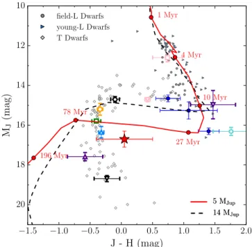
To compute the chi-squared between the spectrum of 51Erib and the objects within the library, we use two different equations. The first method permits each individual filter spectrum to vary freely (unrestricted fit). In the unrest-ricted fit, we compute the_{c statistic for the jth object within}2 Figure 5.The brown dwarf and imaged exoplanet color–magnitude diagram. 51Erib is shown with the red star. The colors of 51Erib place it among late-T dwarfs, where it is redder than most comparable-temperature brown dwarfs, likely indicative of greater cloud opacity in the atmosphere. The photometry for the field M-dwarfs (black circles), young M-dwarfs (blue triangles), field L-dwarfs (dark gray circles), young L-dwarfs (light blue triangles), and T-dwarfs (light gray circles) is taken from the compilation of Dupuy & Liu (2012)and Liu et al. (2016)_{. We used a linear fit to convert WISE W1 photometry to L}P, similar to what was done in

Macintosh et al. (2015). The photometry for the directly imaged planets and young brown dwarfs were taken from Males et al. (2014), Bonnefoy et al. (2014), Bowler et al. (2017), Marois et al. (2010), Chauvin et al. (2005), Rameau et al. (2013), Naud et al. (2014), Leggett et al. (2007), Delorme et al. (2017), Goldman et al. (2010), Janson et al. (2011), and Kuzuhara et al. (2013).

the library as S F C S F _{, 1} j i i i j i j T i i i j i j 2 1 4 , , 1 , ,

å

where Si is the spectrum of the planet, Ci is the covariance

matrix calculated in Section6, and Fi j, is the spectrum of the jth comparison brown dwarf, all for the ith filter. For each

object, the scale factora that minimizesi j, c is found using a2

downhill simplex minimization algorithm. In this method, the scale factor for each object,a , is allowed to vary between thei j,

four filters (JHK K1 2). This is equivalent to allowing the near-IR colors to vary freely up and down in order to better fit the object (e.g., Burningham et al. 2011).

In the second method, the individual filter spectra are still allowed to vary, only within the satellite spot brightness ratio uncertainty (restricted fit), thereby restricting the scale factor for each filter. For the restricted fit, the scale factor is split into two components. The first,a , is independent of the filter andj

accounts for the bulk of the difference in flux between 51Erib and the comparison object due to differing distances and radii. The second, b , is a filter-dependent factor that accounts fori j,

uncertainties in the satellite spot ratios given in Maire et al. (2014). Equation (1)is modified to include an additional cost term restricting the possible values ofb :i j,

S F C S F N 1 2 j i i j i j i j T i i j i j i j i i j i 2 1 4 , , 1 , , , 2

å

spectrum for the ith filter, and s is the uncertainty in thei

satellite spot flux ratio given in Maire et al. (2014)for the same filter. The second term in Equation (2)penalizes values of the scale factor,b , that are very different from the satellite spoti j,

uncertainty and thus increases the chi-squared for objects significantly different from 51Erib.

The spectral type of 51Erib was estimated for both fits from the_{c of the L5–T9 near-IR spectral standards (Burgasser et al.}2

2006; Kirkpatrick et al.2010; Cushing et al.2011). To compute the weighted mean and standard deviation of 51Erib, we converted the spectral type to a numerical value for the standard brown dwarfs, that is, L5=75, T5=85. Each numerical spectral type when compared to 51Erib is weighted according to the ratio of its _{c to the minimum}2 _{c for all}2

standards (e.g., Burgasser et al.2010), and the lowest value was adopted as the spectral type of 51Erib. A systematic uncertainty of one-half subtype was assumed for the standards. We find that the two estimates are consistent with one another, that is, T6.3±1.3 and 6.1±1.4 for unrestricted and restricted fits, respectively; see Figure 6. We adopt a spectral type for 51Erib of T6.5±1.5 from the unrestricted fit, rounded to the nearest half subtype.

The best-fit object for both the unrestricted and restricted fits was G204-39B (SDSS J175805.46+463311.9; c =_n2 1.033 and 1.209), a T6.5 brown dwarf common proper motion companion to the nearby M3 star G204-39A (Faherty et al. 2010). G204-39B has marginally low surface gravity based on photometric (logg »4.5; Knapp et al. 2004) and spectroscopic measurements (logg=4.7–4.9; Burgasser et al.

2006), indicative of it being younger than the field population. While the binary system is not thought to be a member of any known young moving group (Gagné et al. 2014), the stellar primary can be used to provide a constraint on the age of the system. Combining the X-ray and chromospheric activity indicators for the M-dwarf primary and a comparison of the luminosity of the secondary with evolutionary models, Faherty et al. (2010) adopt an age of 0.5–1.5 Gyr for the system. 51Erib is redder than the spectrum of G204-39B (Figure7), especially in terms of the H−K color, which is a photometric diagnostic of low surface gravity among T-dwarfs (e.g., Knapp et al. 2004). This is consistent with the younger age of 51Erib, and the most likely cause for this is that it has lower surface gravity than does G204-39B.

Additional good matches to the 51Erib spectrum include

2MASSJ22282889–4310262 (2M 2228–43, c =_n2 1.07 and

1.26 for the two fits) and 2MASSJ10073369–4555147 (2M 1007–45, c =_n2 1.07 and 1.33). 2M2228–43 is a well-studied T6 brown dwarf that exhibits a spectrophotometric variability in multiple wavelengths that is indicative of patchy

clouds in the photosphere (Buenzli et al. 2012; Yang

et al. 2016). 2M1007–45 is a T5 brown dwarf at a distance of 17±2pc (Smart et al. 2013). It was identified by Looper et al. (2007)as a low surface gravity object based on its H2O

J

- versus K/H spectral ratios defined in Burgasser et al. (2006); comparisons against solar-metallicity models imply an age of between 200 and 400Myr (Looper et al.2007).

The best-fit objects for each spectral type between spectral types T4.5 and T7.5 using the restricted fit are plotted in Figure 7. While the quality of the fits were generally good, none of the objects were able to provide a good match across all of the bands simultaneously, being too luminous in either the J or K bands. Differences in surface gravity, effective temperature, or metallicity could be the cause (e.g., Knapp et al.2004). The poor fit to the color of 51Erib is especially

Figure 6.Comparison of L5 to T9 field (gray circles) and young (yellow stars) brown dwarf JHK spectra to 51_{Erib using the reducedc . The standard}2

brown dwarf for each spectral bin is plotted with a red cross (Burgasser et al.

2006; Kirkpatrick et al.2010; Cushing et al.2011). The dashed and dotted vertical lines give the best-fitting spectral type and corresponding uncertainty. Top: Each spectral band of the comparison was allowed to float to find the lowest chi-squared while fitting the planet spectrum. Bottom: The spectrum was allowed to float up or down in flux, but was penalized by the spot ratio uncertainty in each respective band.

apparent in the CMDs plotted in Figure5, with 51Erib having unusually red near-IR colors relative to similar spectral type objects.

4.2. Comparison against Young Brown Dwarfs

Searches for young companions and moving group objects have resulted in detections of several tens to hundreds of million year old L-type brown dwarf and planetary-mass companions as well as the identification of L-dwarf subclasses based on youth (e.g., Allers & Liu2013; Filippazzo et al.2015; Faherty et al.2016; Liu et al.2016). In comparison, there exist relatively few known (or suspected) young T-dwarf brown dwarfs. In Figure 8, we plot the known young T-dwarfs and compare them in a manner similar to what was done above for field brown dwarfs. The chi-squared for the fits is not much better than what is seen for the field dwarfs, which is likely due to the absence of young T-dwarfs of spectral type similar to 51Erib.

The brown dwarf SDSSJ1110+0116 with a spectral type of T5/T5.5 is the best-fitting young comparison object. It has been identified as a bona fide member of the ABDoradus moving group and is thus young (110–130 Myr) and low in mass (10–12 MJup; Gagné et al.2015). The other young field object that

closely matches the near-IR spectrum of 51Erib is the T7 peculiar brown dwarf, CFBDSIRJ2149−0403 (Delorme et al.

2012). CFBDSIRJ2149−0403 was originally suggested to be a member of the ABDoradus moving group, but Delorme et al. (2017) find that the parallax and kinematics of the free-floating object rule out its membership in any known young moving group. However, despite the lack of proof of youth, medium-resolution spectroscopy examining the equivalent width of the KI doublet at 1.25 μmsuggests that the object has low surface gravity and is most likely a young planetary-mass object (2–13 MJup). An alternative solution is that it is a higher mass, 2–40MJup, brown dwarf with high metallicity. CFBDSIRJ2149 −0403 shows stronger methane absorption features in the red end of the H-band spectrum as compared to 51Erib. However, it is worth pointing out that while both young objects, SDSSJ1110

+0116 and CFBDSIRJ2149−0403, are reasonable matches

across the J and H spectra of 51Erib, they appear to be underluminous in the K band. A likely reason for this is that 51Erib is much younger than both of the comparison companions and thus has the lowest surface gravity among the three objects (Burgasser et al.2006).

4.3. A Very Red T6 or an L–T Transition Planet?

Based on the position of 51Erib in Figure5, it appears that the trend of planetary-mass objects having redder colors compared to the field, seen in young L-type brown dwarfs and planetary-mass companions (Faherty et al.2016; Liu et al.

2016), possibly continues for the T-type companions. Note that the K-LP CMD shows little reddening, which is natural if

clouds are causing the effect. The effect of clouds is negligible in the K and LP bands. Across both the near- and mid-IR

CMDs, 51Erib is one of the reddest T-type objects, and within its spectral classification it has the reddest colors. This trend in the 51Erib colors was originally noted in Macintosh et al. (2015), where they compared the LPversus H-LPcolor

for the planet and noted that it was clearly redder than the field. Rather than simply being redder than the field T-dwarfs because of the presence of clouds, we present a second possible

Figure 7.Comparison of the spectra, using the restricted fit, of the best-fitting T4.5 to T7.5 field brown dwarfs to 51Erib. The spectra shown in this figure are a subset of the data plotted in Figure 6. The brown dwarf spectral fits plotted here use the restricted chi-squared equations presented in Equation (2). The T4.5 and T5.0 spectra are from Looper et al. (2007), the T5.5 is from Burgasser et al. (2008), the T6.0 is from Burgasser et al. (2004), the T6.5 and T7.5 are from Burgasser et al. (2006), and the T7.0 is from Dupuy & Liu (2012).

interpretation for the red colors of 51Erib, of the planet still undergoing the process of transitioning from L-type to T-type. This hypothesis assumes that the evolutionary track followed is gravity dependent, with examples for higher mass objects shown in Figure 9. In this scenario, 51Erib transitions at fainter magnitudes than that seen for field L–T transition brown dwarfs, and it has not yet completed its evolutionary transition to reach the blue colors typical of field mid-T dwarfs.

In Figure 9, we replot the J vs. J−H panel from the series of CMDs shown in Figure 5. In addition to the photometry of 51Erib and the field and young brown dwarfs, we also

overplot two low-mass, 5 and 14 MJup, evolutionary model

tracks (assuming hot-start conditions) from Saumon & Marley (2008)and Marley et al. (2012). If the L–T transition is gravity dependent, as multiple lines of evidence now suggest (Leggett et al.2008; Dupuy et al.2009; Stephens et al.2009), then lower mass objects may turn blue at fainter absolute magnitudes than field objects. In Figure9, we show a simple model in which the L-to-T transition begins at 900 K atlogg= (solid red line)4 instead of 1200 K atlogg=5.3(dashed black line). In the case of a M5 Jup planet, the L-to-T transition begins and ends about

one magnitude fainter in the J band than is observed for the field population. Furthermore, the congruence of the spectrum of SDSSJ1110+0116 with 51Erib (Figure8)is interesting as SDSSJ1110+0116 lies just short of the blue end of the field L-to-T transition, although it does so at an absolute magnitude just slightly fainter than the field transition magnitude. While these simple models explain the fainter absolute magnitudes of the transition, their colors are too blue and appear to miss the younger brown dwarf and free-floating planets. Similarly, the models are too blue to match the T-dwarf sequence. Clearly, more sophisticated modeling of evolution through the L-to-T transition, accounting for inhomogeneous cloud cover and a gravity-dependent transition mechanism as well as a range of initial conditions, is required. Testing this hypothesis is difficult and would require knowledge of the true mass of the companion as well as the formation mechanism. If this hypothesis is true, then the only objects that are brighter on the CMD should be higher mass objects. There should not be any lower mass objects above and to the left of 51Erib on the

Jvs. J−H CMD shown in Figure9. Figure 8. Comparison of the spectra of known young T-dwarfs to that of

51_{Erib. Similar to the field sequence, the fits presented here were computed} using the restricted chi-squared. From top to bottom, the four spectra were sourced from Luhman et al. (2007), Naud et al. (2014), Burgasser et al. (2006), and Delorme et al. (2012).

Figure 9. The J vs. J−H brown dwarf and imaged exoplanet color– magnitude diagram reproduced from Figure5. The photometry for 51Erib is shown with the red star. Also plotted on the CMD are the evolutionary tracks for 5 and 14 MJupobjects (Marley et al.2012), with the solid red line and

dashed black line, respectively. The models assume a simple gravity dependence for the initiation of the transition. A few ages for the 5MJup

track have been overplotted. The L–T transition for the 5 MJupplanet starts at

approximately 900 K and 20 Myr, but for a lower-mass planet such as 51Erib, it will occur at younger ages.

5. Modeling the Atmosphere of 51Erib

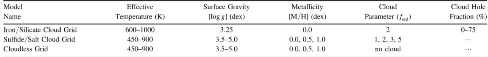
For the purpose of modeling the complete SED of 51Erib, we made use of two updated atmospheric model grids from the same group, focusing on different parameter spaces (see Table 3). The first grid, described in Marley et al. (1996,

2002, 2010), focused on the higher effective temperature atmospheres (L-dwarfs) and includes iron and silicate clouds in the atmosphere. The second grid, described in Morley et al. (2012,2014) and Skemer et al. (2016), is designed for lower effective temperatures (T- and Y-dwarfs) and include salt and sulfide clouds in the atmosphere, which are expected to condense in the atmospheres of mid-to-late-T dwarfs.

The methodology used to fit the models to the data is the same for both model grids. To fit the models to the data, we bin the model spectra to match the spectral resolution of the GPIES spectra across each of the JHK K1 2 filters. For the photometry, we integrated the model flux through the Keck/NIRC2 LPand

MSfilter profiles, respectively. The estimation of the best-fitting

model is done by computing the chi-squared value for each model in the grid compared to the data using Equation (2). We made use of the covariance matrices estimated for the four spectral channels described in theAppendixand also included the variance for each of the two photometric data points to compute the chi-squared statistic. Note that we use the restricted fit equation in the computation of the best-fitting model. This equation permits each of the individual filters to scale within the 1σ error of the satellite spot ratios. We also did the fitting without the scaling factor and found that the results are similar.

As stated in Section2.1.1, the use of the covariance affects the model fitting where the peak of the posterior distribution occurs at slightly cooler effective temperatures, consistent within the errors. Due to the high spectral correlation in the J band (see Figure 19), when using the covariance, the best-fitting models are not models that pass through the data but rather models that have lower flux in the J band than the data. We present the specific modeling details in the following text.

5.1. Iron and Silicate Cloud Models

In Section 4.3, we suggested that 51Erib, rather than having completely evolved to T-type, could be transitioning from L to T. In this scenario, the cloud composition of the planetary atmosphere might still be influenced by the deep iron and silicate condensate grains and patchy cloud atmosphere. Therefore, we compared the planet SED to a grid of models with a fixed low surface gravity and solar metallicity, where the key variable is the cloud hole fraction, and the unique aspect of this grid is the presence of iron or silicate clouds in an atmosphere with clear indications of methane absorption. The clouds are modeled using the prescription presented in Ackerman & Marley (2001), where cloud thickness is parameterized via an efficiency factor ( fsed). Small values of

f_sed indicate atmospheres with thick clouds, whereas large

values of f_sedare for atmospheres with large particles that rain out of the atmosphere, leaving optically thinner clouds. As mentioned earlier, the primary condensate species in this grid are iron, silicate, and corundum clouds, molecules that are expected to dominate clouds in L-dwarfs (Saumon & Marley 2008; Stephens et al. 2009). At the L–T transition, clouds are expected to be patchy, so for each Teff, the models

went from fully cloudy, with f_sed =2 and 0% holes, to an atmosphere with f_sed = and 75% holes (patchy clouds). The2 methodology used to calculate the flux emitted from the patchy cloud atmosphere includes both cloud and cloud-free regions simultaneously in the atmosphere using a single global temperature–pressure profile and is not created via a linear combination of two models, as is sometimes done in the literature (Marley et al.2010). The iron and silicate cloud grid models use solar metallicity (Lodders 2003). The opacity database used for the absorbers are described in Freedman et al. (2008), including updated molecular line lists for ammonia and methane (Yurchenko et al. 2011; Yurchenko & Tenny-son2014). The models span effective temperatures from 600 to 1000 K for solar metallicity ([M/H] = 0.0) and low surface gravity (logg=3.25, 3.50; see Table3).

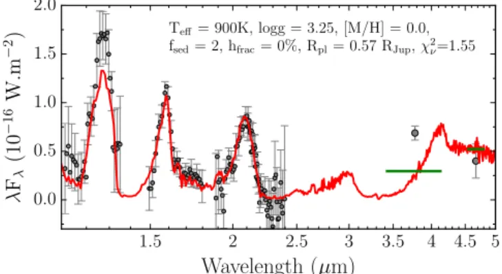
Presented in Figure10is the best-fitting model to the SED of 51Erib. Stated in the figure are the model parameters along with the radius of the planet required to scale the model spectrum to match the planet SED. This scaling factor is required since the model spectra are typically computed to be the emission at the photosphere or at 10 pc from the object. One of the free parameters in most model fitting codes is the term

R2/d2to scale the model flux to match the SED, where R is the radius of the planet and d is the distance to the object. For 51Eri, the distance is known to better than 2% (see Table2), so we only fit the radius term. Shown in Figure 11 is the posterior distribution for the radius, where we find that the best-fitting radii are significantly smaller than that predicted by evolutionary models, for example, 1.33–1.14 RJup for a

2–10MJup hot/cold-start planet at the age of 51Eri (Marley

et al. 2007; Fortney et al. 2008). This discrepancy has been noted previously as well for the HR8799 planets (Marois et al. 2008; Bowler et al. 2010; Barman et al. 2011; Currie

et al. 2011; Marley et al. 2012), βPicb (Morzinski

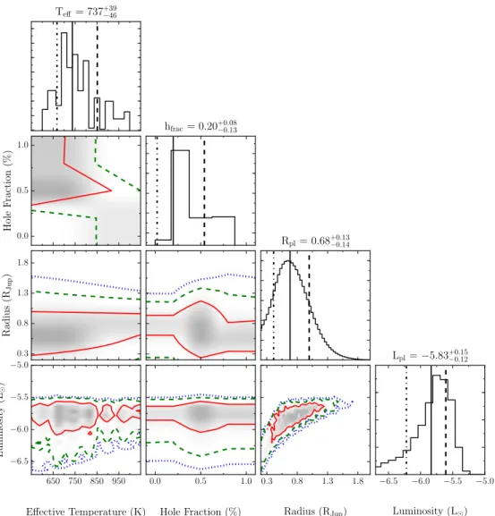
et al. 2015), and for 51Erib itself in the discovery paper (Macintosh et al.2015). In an attempt to circumvent this issue, while modeling the SED we adopted a Bayesian prior probability density function for the radius in the form of a Gaussian centered on the expected radius from evolutionary models (green line in Figure 12), with the width chosen to include the radius of Jupiter. Without the prior (i.e., using a uniform prior), the median radius is 0.68 RJupand Teff ~740K;

with the prior, the median radius value is forced closer to the predictions of evolutionary models (red line in Figure 12) at 0.98 RJupand Teff∼690 K, biasing the luminosity of the planet

Table 3 Model Grid Parameters

Model Effective Surface Gravity Metallicity Cloud Cloud Hole

Name Temperature (K) [log ] (dex)g [M/H] (dex) Parameter ( fsed) Fraction (%)

Iron/Silicate Cloud Grid 600–1000 3.25 0.0 2 0–75

Sulfide/Salt Cloud Grid 450–900 3.5–5.0 0.0, 0.5, 1.0 1, 2, 3, 5 L

to larger values. When fitting the SED, the term that is conserved is the luminosity rather than the effective temper-ature or the radius. Adopting the evolutionary radius and marginalizing over the uncertainty in radius raises the luminosity (logL L) from −5.83 to −5.65. Since

observa-tional constraints on the radius for young planets are unavailable, we chose to use an uninformative prior.

Plotted in Figure 11 are the normalized posterior distribu-tions for each of the model parameters varied in the model fit, along with the covariances to show how each of the parameters are affected. Since the grid only had a few models with

g

log =3.5, with the majority being 3.25, we marginalized over the surface gravity. The irregular shape of the effective temperature posterior is caused by the missing models in the grid. The median effective temperature, 737K, estimated from the grid falls right in between the range of best-fitting temperatures from the models in the Macintosh et al. (2015) paper (700–750 K). However, based on the shape of the posterior and the covariances, the peak of the effective temperature distribution extends to cooler temperatures. Since the L-to-T transition has been suggested to arise from holes or low-opacity patches appearing in an initially more uniform cloud deck (Ackerman & Marley2001; Burgasser et al.2002; Marley et al.2010), our finding here that partly cloudy models best fit the 51 Eri b spectrum is consistent with this interpretation. In general, however, the models struggled to fit the entire planet SED, typically being able to fit either the near- or mid-IR portions of the SED. The inability to fit mid-IR photometry suggests that chemical equilibrium models are not appropriate. Disequilibrium chemistry predicts less CH4in the atmosphere and could explain the higher flux at 1.6 μmand in the LP band. It would also introduce CO, accounting for the

lower flux in the MSband.

5.2. Sulfide and Salt Cloud Models

In Section4.1, we showed that the best-fitting spectral type of 51Erib is a mid-to-late-T dwarf. At the effective temperatures of mid-to-late-T dwarfs, Cr, MnS, Na2S, ZnS, and KCl are expected to condense and form clouds high in the photosphere. The second grid we tested the planet SED against made use of a model grid that includes salt and sulfide clouds to test additional parameters such as the surface gravity and metallicity (which were varied, unlike the iron/silicate grid) and the properties of clouds typically associated with T-dwarfs. The grid was designed specifically for lower temperature objects (450~900K; Morley et al.2012,2014)and has been

used successfully to reproduce the SED of GJ504b (Skemer et al.2016), a cool low-mass companion with a similar spectral type (late-T) that is comparable to 51Erib (Kuzuhara et al. 2013). Note that the use of this cloud grid does not preclude the possibility of the planet transitioning from L to T. Also included as part of this grid are the clear atmosphere models from Saumon & Marley (2008), the ranges for which are presented in Table3. The ranges of parameters varied are presented in Table3, including temperatures, surface gravities, metallicities, and sedimentation factor ( f_sed) ranging from cloudy ( f_sed=1) to cloud-free. The cloud model used in the sulfide/salt grid is the same as the one described above. In addition to the opacity updates mentioned above, opacity effects due to alkali metals (Li, Na, K) have been included using the results from Allard et al. (2005). For effective temperatures between 450 and 775 K, the grid is complete with models available for every step of the varied parameters. For effective temperatures between 800 and 900 K, the temperature steps switch from increments of 25–50 K, and there are no models with f_sedvalues of 1 and 2. This grid does not include the opacity effect that is due to iron and silicate condensates. A future series of papers describing an extended atmosphere model grid will describe the updates, but the present grid extends the models to greater than solar metallicities.

In Figure 13, we present the four best-fitting model

atmospheres for 51Erib. Presented in each panel are the atmosphere with the lowest reduced chi-squared in one of four cases, namely, solar and cloudless (top left), solar and cloudy (top right), nonsolar and cloudless (bottom left), and nonsolar and cloudy (bottom right). Both cloudless model atmospheres are warmer and thus fit the near-IR spectrum of the planet while completely missing the LPphotometry. The cloudy atmosphere

model fits are cooler and do a much better job of fitting the overall SED of 51Erib, and the best-fitting atmospheres for both solar and nonsolar metallicity have very similar reduced chi-squared values.

The normalized posterior distributions for the different parameters varied as part of the model fitting are shown in Figure 14. The best-fitting Teff (605-+6661 K) is much cooler in

comparison to the iron/silicate grid, but the values are within 2σ of each other. We also note that the median might not be the best estimate for the effective temperature PDF in the iron/ silicate grid where the peak extended to cooler temperatures. For the surface gravity and metallicity posterior distributions, we present the median values and error bar assuming a Gaussian distribution, though they may not be Gaussian. The surface gravity PDF suggests that the planet has high surface gravity. However, 51Erib is clearly a low-mass companion, indicating that the data do not constrain the gravity. A prior might help constrain the distribution, but there are currently no physically motivated priors available for the surface gravity of young planets. Similarly, the PDF for the metallicity is also unconstrained, and higher resolution spectra in the K band might help provide greater constraints on the metallicity of 51Erib (Konopacky et al.2013).

A difference between the iron/silicate and salt/sulfide atmosphere grids is in the planet radius, where the best-fit radii for the cloudy models and the median radius of the PDF for the salt/sulfide models are much closer to evolutionary model predictions. A possible explanation for this discrepancy is that fitting the lower effective temperatures while still matching the bolometric luminosity requires a larger radius. If

Figure 10.Spectral energy distribution of 51Erib with the best-fitting iron and silicate cloudy model.

the iron/silicate models extended to lower temperatures, assuming the continued presence of these clouds at these colder temperatures, it is likely that the radius discrepancy would not be as apparent. The sedimentation factor was fixed (at f_sed = ) in the iron/silicate grids but had varying hole2

fractions (hfrac). In the sulfide/salt grid, fsed was varied, and

the median value for the distribution is f_sed =2.48. If we equate the hfracfrom the iron/silicate model with the fsedas the

physics controlling the emission of flux from the photosphere, then for both model grids the best-fitting models tend to favor the presence of clouds over cloud-free atmospheres. Further-more, in both cases, the best-fitting models were not the fully cloudy atmospheres, with the smallest hfrac/ fsed. While the

cloud compositions in both models are different, fitting either grid requires the cloud opacity. This can be achieved in one of two ways: either make the deep iron/silicate clouds be very vertically extended (small f_sed)or introduce a new cloud layer in the form of the sulfide/salt clouds.

The cloudy model atmosphere fits presented in Figure 13

match the H through K spectrum while being slightly underluminous in the J and overluminous MS bands. Given

the large photometric errors in the MS data, the model

photometry lies within 2σ of the data. JWST and other future low-background mid-IR instruments will better constrain the 3–24μmSED, a further test of current models. In Figure15, we show 10 of the best-fitting models assuming cloudy (sulfide/salt clouds) or cloudless atmospheres extended out to 20 μm. It is clear from these models that observations with the

Figure 11.Normalized posterior distributions for the iron and silicate model grid. The PDFs are for the parameters varied in our fit along with the inferred distribution of the luminosity of 51Erib. The lines on the 1D histogram indicate the 16th, 50th, and 84th percentile values, while those on the 2D histogram are the 1σ (solid red), 2σ (dashed green), and 3σ (dotted blue) values of the distribution. The values printed above each histogram are the median value along with the 1σ error on it.

Figure 12. The figure shows the effect of applying a Gaussian radius prior when modeling with the iron/silicate grid. The prior shown by the green line is centered on the radius given by evolutionary models: 1.29 RJup(Marley et al.

2007; Fortney et al.2008). Also plotted are the likelihood (black) and posterior distribution (red).