Approximations for Manufacturing Networks
of Queues with Overtime
Gabriel R Bitran*t
Devanath Tirupati**
WP# 2519 1
was 1919-89
March 1989
*Sloan School of Management, Massachusetts Institute of Technology
**Department of Management, University of Texas at Austin
tThis research has been partially supported by the
Leaders for Manufacturing Program.
Approximations for Manufacturing Networks of Queues with Overtime
Gabriel R. Bitran* and Devanath Tirupati**
Abstract
In this paper we present simple approximations for networks of queues with overtime operation at some stations. This type of network is
commonly encountered in practice in several manufacturing applications. We provide bounds on the performance of the approximations for single
and multiple machine stations. Our results suggest that the methods perform satisfactorily. These approximations can be used in conjunction with the parametric decomposition methods to analyze queueing networks. The computational results indicate that the performance of the
decomposition approach does not deteriorate when combined with the methods proposed in this paper.
* Sloan School of Management, Massachusetts Institute of Technology ** Department of Management, The University of Texas at Austin.
Approximations for Manufacturing Networks of ueues with Overtime
1.0 Introduction:
Queueing network models have been used to model a variety of
systems in computer and communication networks, service facilities, and discrete and flexible manufacturing systems. However, exact results for analysis of such systems is limited to product form networks (see
Jackson 1963; Kelly 1975; Baskett et.al. 1975; and Lemoine 1977). For more general systems, the focus has been on the development of
approximations and simulation methods. In the analysis of manufacturing systems modeled by open networks of queues, the parametric decomposition method has been used with good results, among others, by Shanthikumar and Buzacott (1981), Whitt (1983) and Bitran and Tirupati (1988a). This approach generalizes the notion of independence and product form
solutions of Jackson type networks. In this method, the arrival process at each station is approximated by a renewal process and the squared coefficient of variation (scv) of interarrival times at each station is computed approximately. Performance measures such as the mean number of jobs and queue lengths at each station are estimated based on two moment
approximations. For a detailed description of this approach see Whitt (1983), Bitran and Tirupati (1988a) and references therein. Recently, Bitran and Tirupati (1988b) have extended these methods to certain types of batch operations encountered in manufacturing systems. Segal and Whitt (1988) describe a new version of the queueing network analyzer
that incorporates several features found in manufacturing lines. These include machine breakdowns, changing lot sizes, product testing with partial yields etc.
A feature of manufacturing systems that is not usually considered (at least explicitly) in queueing network models is the use of overtime. It is common to encounter plants where relatively heavily utilized
stations work more hours per day than others. Also, in stations with multiple machines, the number of machines that operate during overtime
is not necessarily the same as that used during regular time. Job releases to the shop, subsequent movement between stations, and departures from the system usually take place during regular hours.
In theory, such situations can be modeled as nonstationary systems. However, the exact analysis is extremely complex, if not impossible. The focus of the research on nonstationary queues has been on describing
the time dependent behavior (for example, see Rothkopf and Oren 1979; Keller 1982; and references therein) and asymptotic behavior of the
system (see Lemoine 1981; Wolff 1982; Heyman and Whitt 1984 and references therein). These results do not provide a mechanism to
estimate performance measures such as the mean number of jobs, and mean waiting times in networks of queues with features described in the previous paragraph.
In this paper our objective is to present simple approximations that can be used in the context of networks of queues to model stations with overtime. In stations with multiple machines, we consider cases in which only some machines work overtime. We provide bounds on the
performance of the approximation for single and multiple machine stations. For multiple machine stations, our results suggest that in most practical situations, the approximation is likely to be robust. These conclusions are supported by computational experiments reported in Section 3. One of these examples is a network with 13 stations and 10
products that is based on a semiconductor facility producing specialty devices. In addition, our computational results suggest that the parametric decomposition methods are fairly robust in the analysis of such systems.
The remainder of the paper is organized as follows. In the next section we present the approximations and the related results. In Section 3 we describe the computational experiments. In Section 4 we conclude with comments on the scope of these approximations.
2.0 Approximations to Model Stations with Overtime 2.1 Approximation for a Single Machine Station:
Consider a single machine station (System A) with the following characteristics:
(i) The machine is available for r hours of regular time every day.
(ii) The machine is available for ov hours of overtime every day, i.e., the total availability is (r+ov) hours per day.
(iii) Jobs arrive at the station at a rate per day with all arrivals taking place during regular time only.
(iv) Jobs that are completed during regular time leave the station immediately upon completion.
(v) Jobs that are completed during overtime leave the station at the beginning of the following day.
(vi) First come, first serve discipline (FCFS) is observed at the station.
III
ai (dai, tai): arrival time of the it h job; dai represents the day and tai the hour of arrival of the ith job.
bi: service time of job i (in hours). Let b denote the mean service
time.
di (ddi, tdi): departure time of the ith job; ddi and tdi
represent respectively the day and hour of the departure epoch for the ith job.
p: utilization = Ab/(r +ov)
We propose an approximate analysis of system A by analyzing a related single machine system Al with the following characteristics:
(i) The machine is available for r regular hours per day. (ii) The pattern of job arrivals is identical to that of system
A, i.e., ai' = ai for all i, where ai' represents the
arrival epoch of the ith job in system Al.
(iii) The service time of the ith job, bi', is scaled as follows bi = kbi, where k = r/(r+ov), i = 1, 2, ...
(iv) All jobs leave the system immediately upon completion of service.
(v) The priority discipline is FCFS.
Let ai ' = (dai', tai'), di' = (ddi', tdi'), bi' and p' denote the
corresponding variables in system A1.
di - x, di' - x: denote a time x hours before the departure of job i in system A and A respectively.
di + x, di' + x: denote a time x hours after the departure of job i in system A and Al respectively. Idi - di'l < x indicates that the departure times of job i in A and Al are within x hours.
The primary motivation for the approximation above follows from -the fact that the service or processing rate measured as the number of jobs per day is the same in both systems A and Al. Hence, as long as the systems are busy, the amount of work completed in the two systems during an integral number of days are equivalent. The method has other
advantages as well. First, the utilizations in the two systems A and A1 are the same, i.e., p' = p. This is important since, in most queueing systems, utilization is a major determinant of the performance measures. Second, the approximation is easy to apply in a network of queues. By applying this procedure at all stations, we obtain a related network in which all stations work the same hours. This system can be analyzed by conventional methods using either exact or approximate methods or
simulation. Proposition 1 below suggests that the approximation is likely to be robust, particularly when the utilization is high.
Definition: A sample path is defined as a sequence of job arrivals with associated service times.
Proposition 1: In every sample path, the departure instances of
corresponding jobs in systems A and Al do not differ by more than k ov. Specifically, this implies the following:
(i) If job i is completed during regular time, i.e.,
0 < tdi r, then di'e d*, d**), where d* and d** are defined as follows:
d* : (ddi-l, r-k ov+tdi) if tdi<k ov (ddi, tdi-k ov) otherwise. d**: (ddi, tdi+k ov) if tdi<r-k ov
(ii) If the ith job is completed during overtime in system A then either ddi = ddi' and tdi 0, and tdi' < k ov;
or ddi ddi' + 1 and tdi D 0, and r - k ov < tdi'~ r.
We denote the above result as di - di'I < k ov. (The proof of the proposition above is in Appendix 1.)
When both systems A and Al are busy, equivalent amount of work is completed (in the two systems) over any interval spanning an integral number of days. Proposition 1 describes one consequence of this fact which suggests that the performance measures in system A may be
estimated from the corresponding measures in Al. For example, the error in estimating mean waiting time is not greater than k ov hours. (If the waiting time is measured in days, the error is not greater than k ov/r days.) The application of Little's law provides a corresponding error bound on the mean number of jobs. As a result, if the utilization is high and the average waiting times are large, the relative error in measuring the mean waiting time and the mean number of jobs is likely to be small.
Corollary 1: In a system where the interarrival times are independent and identically distributed (iid), service times are iid and utilization p < 1, so that we have steady state, the relative error in estimating the mean number of jobs tends to zero as p 1.
This is an encouraging result. As we observed earlier in Section 1, we expect stations with relatively high utilization to work overtime. Corollary 1 suggests that in those cases the approximation is good. When the utilizations are low and the waiting times are small, we expect that the absolute error in the estimates of the mean number of jobs will
not be significant. This fact was also observed in computational experiments not reported in this paper for brevity.
2.2 Multiple Machine Station:
Consider a m machine work station (system B) with the following characteristics:
(i) The station operates with m machines on regular time for r hours each day.
(ii) The station operates ov hours of overtime each day with m2 m machines.
(iii) A FCFS discipline is observed.
(iv) Jobs completed during overtime depart from the system the following day, while those that are completed during regular
time leave immediately upon completion of service.
As an approximation to system B, we propose a m machine station (system B1) with the following characteristics:
(i) The station operates with m machines during regular time of r hours each day.
(ii) The service times are scaled as bi ' klbi
where k = mlr/(mlr + m2ov)
(iii) The priority scheme is FCFS and jobs leave the system immediately upon completion.
Observe that the service rate (measured with days as the unit of time) is (r + ov)/b jobs per day for the m2 machines that work over
time, while it is r/b for the remaining machines that only work regular hours. In system B all machines have a processing rate of r/(klb) so that the aggregate processing rate in the two systems is the same. The motivation for the approximation follows from the fact that if all the
machines are busy, i.e., the number of jobs is not less then ml, an equivalent amount of work is completed in the two systems over any interval that spans an integral number of days. The approximation has other advantages similar to those for the single machine case. Both systems B and B1 have the same utilization, and the use of B permits analysis of networks using conventional methods. When all machines work over time, i.e., m2 - ml, the results of proposition 1 hold for this approximation as well.
Proposition 2: Suppose that m2 = m and all machines work overtime in system B. Then in every sample path, the departure instances of
corresponding jobs in systems B and B do not differ by more than k ov, i.e., Idi - di'I k ov.
The proof of this proposition is in Appendix 1.
Observe that, in general when m2 < ml, B1 involves approximations in two dimensions -- in the number of machines and the hours worked. Hence, we expect that the approximation will be weaker than that for the single machine station. The following example suggests that in any sample path it is possible for individual jobs to have corresponding departure times (in systems B and B) arbitrarily apart.
Example: Consider a job that arrives at the station (in system B) when the system is empty. Let the process time for the job be b hours. This represents a processing requirement of b/(r + ov) days. In system Bl the corresponding process time is b' = klb hours, which in turn
corresponds to {ml/(mlr + m2ov) } b days of work.
Note that (ml/(mlr + m2ov)) b = {ml(r+ov)/(mlr + m2ov)) [b/(r+ov)]
> b/(r+ov), if m2 < ml and ov > 0.
Even if the waiting time for the job is zero in system B (same as in B), the difference in departure epochs (measured in days) in systems B and B1 can be made arbitrarily large by choosing a correspondingly large b. This difference will increase further if the job has to wait in B1.
The example suggests that system B may not be a good approximation for specific jobs. However, we note that when the number of jobs in the system is not less than m at any point in time, the work content in the two systems would be close. Also in that case the work completion rate on a daily basis will be the same in both systems.
Lemma 1: Consider a multimachine station with m2 < ml. Assume that the job arrivals and service times are such that the number of jobs in
systems B and B are at least ml at any point in time. Then in every sample path,
wk(t) - (mlr + m2ov) wk'(t) m2ov
mlr
where wk(t), and wk'(t) respectively represent the unfinished work
content in systems B and B. The unfinished work content is measured as the hours of processing required to complete the jobs in process and those in queue in the respective systems.
Furthermore, if t is integral in number of days, k wk(t) = wk'(t). Lemma 1 provides an error bound on the estimates of the work
content wk(t). However, we note that it is not easy to obtain similar bounds for the number of jobs. With m2 < ml, the processing rates
(measured as number of jobs per day) is not identical for all machines in system B, and can result in the assignment of jobs to different machines in the two systems. While the amount of work completed in B
and B1 are nearly equivalent, the number of jobs processed depends on sequencing and priority rules used during overtime operation. In Remark 1 below, we provide a parametric bound on the difference in the number of jobs in relatively heavily utilized systems. This bound depends on the ratio of maximum and minimum process times, and in some sense, represents a worst case error bound on the performance of the approximation.
Remark 1: Consider a multimachine station with m2 < ml. Assume that
the job arrivals and service times are such that the number of jobs is at least m in both systems B and B at any point in time. Also assume
that at time t = 0, the processing of first job is initiated in both systems B and B. Let b* = bmax/bminJ, where bmax and bmin
respectively denote maximum and minimum process times. Consider systems B and B at the start of any day, i.e., at any point in time T, where T
is integral in number of days. The number of jobs in the two systems do not differ by more than (ml - 1) (b* + 1) - 1. (See Appendix 1 for proof of this assertion.)
These results are encouraging. Since in most manufacturing systems overtime is used only when there are waiting jobs, we expect that in most practical cases at stations that work overtime, the mean number of jobs will not be small and the approximation should be adequate. The
results of the computational experiments described in the next section support this conjecture.
3.0 Computational Results:
We examined the quality of the approximations proposed in this paper by comparing estimates of the mean number of jobs (at each
station) in a series of five experiments. In the first four experiments
we considered single product systems and tandem queues with two and three stations. In two cases we had stations with single machine and in the other two we tested problems with multiple machines. In the last experiment we considered a network derived from a semiconductor facility producing specialty devices. It consists of 13 single machine stations and 10 product classes. A secondary objective of the computations was to evaluate the robustness of the parametric decomposition approach
(together with the approximations of this paper) in estimating the mean number of jobs in systems with overtime at some stations. These
approximations are based on Shanthikumar and Buzacott (1981), Whitt (1983, 1985), and Bitran and Tirupati (1988a) and are summarized in Appendix 2. Since exact solutions are not available for most of the
test problems, we used simulation as a benchmark. This is a common practice in evaluating queueing approximations. (For example, see Albin
1984, Whitt 1985, and Bitran and Tirupati 1988a.) In the design of the test problems the squared coefficient of variation (scv) of interarrival and service times were chosen not greater than one. This choice was motivated by our experience in manufacturing systems in which the corresponding scvs are typically smaller than one.
3.1 Experiments in Networks with One-machine Stations: In the first experiment we considered a single product, two station tandem queue shown in figure 3.1. The work schedules at the two stations were
different. While station 2 operated a regular time of 8 hours each day, station 1 was available for additional (overtime) operation each day. The objective of this experiment was two fold. First, we examined the quality of approximations of section 2 in estimating the mean number of jobs at station 1. Second, we examined the impact of overtime operation
III
on the estimates at station 2. We expect that the impact on stations further downstream would be even less significant. In the design of the test problems we considered the following factors:
(i) Overtime operation at station 1: We considered three levels of overtime -- 0, 1 and 2 hours each day. The availability varied from 8 to 10 hours per day. These systems are
denoted as (8,8), (9,8) and (10,8) respectively.
(ii) The arrival rate was set at 1 job per day (mean interarrival time 8 hours). Experiments in which the arrival rates are larger than one are described in Section 3.3. Job arrivals take place during regular time hours only. The interarrival times were assumed to have independent and identical
distributions (iid). We considered two distributions --exponential and second order Erlang for interarrival times. (iii) Service times at each station were assumed to be iid. We
considered two distributions for service times
--exponential and second order Erlang. In these problems, the service time distribution was the same at both stations. (iv) The utilization at station 2 was set at 0.8. At station 1
we considered two levels of utilization; 0.75 and 0.85. Note that station utilization together with the number of hours of operation and choice of distribution (Erlang or exponential) completely specifies the service time
distribution at each station.
The number of test problems in this experiment was 24. The simulation estimates of the mean number of jobs is presented in Table 3.1. The table also presents the corresponding estimates by the
decomposition approach using the approximations of this paper. These results are very encouraging. First, note that the variation in the mean number of jobs with overtime level is not significant. Case (a) in Table 3.1 represents the proposed approximation for systems (b) and (c). The estimates of (a) compare very well with those of (b) and (c) which
suggests that the approximation adjusting for overtime operation should be adequate in most practical situations. Also note that the impact of overtime on the mean number of jobs at station 2 is also insignificant. The approximations for estimating the number of jobs seem to be very
effective. The table also provides, for each problem, the maximum of the absolute relative errors in estimating the mean number of jobs in systems (a), (b) and (c) using the decomposition methods. These errors range between .88% and 7.06% and are typical of the decomposition
approach. These results suggest that the performance of the decomposition method does not deteriorate when combined with the approximation of Section 2.1.
The simulation estimates reported in the table are based on six batch runs of 100,000 jobs each and represent the average of 600,000 jobs. We felt that these runs were sufficiently long to provide
representative estimates. To illustrate the accuracy of the simulation estimates we present, for two of the test problems, the standard
deviation of the six batch estimates for the mean number of jobs. The two examples correspond to the following cases:
Example 1: System (10,8); Pi = 0.85; Erlang distribution for interarrival and service times.
Example 2: system (9,8); P1 = 0.75, Exponential distribution for
Ill
The standard deviations of the mean number of jobs for the first example were .0512 and .0293 at stations 1 and 2 respectively. The corresponding figures for the second example were .0429 and .0766.
These figures are representative of the results obtained. Note that the differences in the mean number of jobs with varying overtime is of the
same order as the standard deviation of the simulation estimates. This again suggests that these variations are insignificant.
In the second experiment we considered a three station network shown in figure 3.2. The objective in this test was to examine the quality of the proposed approximation with a wider variation in the operating schedules. We simulated the test problems with the following schedules:
(a) All 3 stations working 8 hours per day (no overtime). This is denoted by (8,8,8).
(b) The first and the third stations work 8 hours each day while the second works 10 hours; (8,10,8).
(c) First station works 6 hours, second 10 hours and the third 8 hours per day; (6,10,8).
(d) The three stations work 8, 10 and 6 hours respectively; (8,10,6).
These cases represent a wide variation in operating hours that accommodate many manufacturing applications. (Note that the ratio of maximum to minimum working hours is 1.67.) Observe that system (a) above is the proposed approximation for systems (b), (c) and (d). For each of these systems we simulated 4 test problems with the following parameters.
(i) The arrival rate was 1 job per day. (Experiments in which the arrival rates are larger than one are described in section 3.3). The interarrival times were assumed to be
iid. We considered two alternative distributions --exponential and second order Erlang.
(ii) Service times at each station were assumed to be iid. We considered two distributions for service time -- exponential and second order Erlang. Again in each problem, the scv of service time was the same at all stations.
(iii) The utilization at stations 1 and 3 was set at 0.8, while at station 2 it was set at 0.85.
The computational results for the 16 cases are presented in table 3.2. It is clear from these results that (a) is indeed a very good approximation for (b), (c) and (d). The variation in the simulation estimates is small. (It is of the same order as the standard deviation of the batch results.) The performance of the approximation is also encouraging. The table presents the maximum absolute relative error in
estimating the mean number of jobs in systems (a), (b), (c) and (d) using the decomposition method. These errors range between 1.25% and
8.27%. Again, the simulation estimates are based on six batch runs of 100,000 jobs in each run and the accuracy is similar to those in the first experiment.
3.2 Experiments in Tandem Networks with Multiple-Machine Stations: In this section we report the results of tests in networks with multiple machine centers. The network for the first experiment was the two station system of figure 3.1. The number of machines at stations 1 and 2 was 3 and 2 respectively. Station 2 operated on regular time schedule
III
of 8 hours per day and we considered three levels of overtime at station 1. During overtime operation only 2 machines were available at this station. Thus, we had the following three systems defined by the overtime levels.
(a) No overtime and both stations work 8 hours per day. This is denoted by (8,8).
(b) Overtime of one hour per day at station 1, i.e., system (9,8). (c) System (10,8) with two hours of overtime at station 1.
For each system we simulated four problems by varying the distribution of interarrival and service times. The alternative distributions considered were similar to the test problems in Section 3.1 and consisted of exponential and second order Erlang distributions. In all test problems the utilization at station 1 was 0.85 and 0.8 at station 2. Observe that system (a) represents our proposed
approximation for systems (b) and (c). In these experiments, we implemented the FCFS discipline in the following manner. When the number of jobs in the systems was not greater than m all the jobs are processed during overtime. When the number of jobs was greater than ml, the machines that were processing the first m2 jobs (jobs with the
highest priority) work overtime.
The results presented in Table 3.3 support conclusions similar to those observed in the single machine experiments of Section 3.1. The mean number of jobs at each station in systems (a), (b) and (c) are very close and well within the accuracy of the simulation estimates. This suggests that the proposed approximation is very reasonable. Table 3.3 presents for each problem, the maximum percentage error of the absolute deviation of the approximation from the simulation results. These
errors range from 1.36% to 6.69% which is acceptable in most applications.
The simulation estimates in this experiment are based on twelve batch runs with 50,000 jobs in each run. We felt a total of 600,000 jobs was sufficient to provide good estimates. To illustrate the accuracy of these results, we provide the standard deviation of the batch estimates for the following two cases:
Example 1: System (c); distribution of interarrival and service times are Erlang.
Example 2: System (b); interarrival and service time distributions are Erlang and exponential respectively.
In the first example, the standard deviation of the mean number of jobs was .0716 and .0991 at stations 1 and 2 respectively. The
corresponding figures for the second case are .1291 and .0676. The three station system of Figure 3.2 was the network for the second experiment. The number of machines was 2 at stations 1 and 3, and 3 at station 2. The design of the test problems was similar to the previous experiments. Station 2 had overtime operation while the other two worked during regular time hours only. Also, during overtime only two machines were used. We defined three systems with varying overtime levels. These are (a) (8,8,8) -- No overtime. All stations work 8 hours; (b) (8,9,8) -- overtime of 1 hour at station 2; and (c) (8,10,8) -- overtime of 2 hours at station 2. As in the previous experiments, for each of these systems we tested four problems by varying the
distribution of interarrival and service times. The utilizations were set at 0.8, 0.85 and 0.8 at stations 1, 2 and 3 respectively.
Ill
The results presented in table 3.4 support the conclusions of the previous experiments. Observe that estimates from system (a) would be a very good approximation for systems (b) and (c). The differences in the simulation figures are not significant. The approximations continue to perform well. The range of the maximum percentage absolute error
(relative to the simulation values) was 0.69% to 8.00%. These errors are typical of the parametric decomposition approach in the analysis of general networks. It is interesting to note that differences between estimates in column (d) and columns (a), (b), (c) are comparable. Hence it appears that the performance of the decomposition approach when
combined with the approximations proposed in Section 2.2 does not deteriorate.
3.3 A Network Example: In this section we describe an experiment with a network that models the manufacturing facility of a semiconductor company producing specialty semiconductor devices. The facility consisted of 13 single machine stations and processed jobs classified into 10 product families. The routing for jobs in each class was deterministic and described in Table A3.1 of Appendix 3. Observe that the number of operations for each job is between 7 and 13 and a job returns to the photolithography department (station 2) several times. The arrival rate of jobs in each family was 1 per day and the
distribution of interarrival times are presented in Table A3.1. The resulting net arrival rates at the stations in the network range from 3 to 25 jobs/day. The station data consisting of operating schedule, utilization and process time distribution is described in Table A3.2. Note that the service time distribution is completely specified by this data together with the net arrival rate computed from product data.
Table A3.2 also specifies an averar- dollar value (vj) for each job at station j. The work-in-process (wip) at station j is measured as the product of vj and the mean number of jobs (Lj). The total wip in the system is obtained by adding the station wips. Observe that the work schedules of the stations in the network vary considerably. For
example, stations 1, 4 and 6 work only regular time hours while 8 and 12 operate more than 10 hours. These variations are typical of many
manufacturing systems. We refer to this as system (a).
In Table 3.5 we present three estimates for the mean number of jobs at each station and total system wip. Estimates (a) in the table are based on simulation of the network described by Tables A3.1 and A3.2. Estimates (b) are obtained by simulating the network derived by applying the approximations presented in Section 2. In this network all stations work the same schedule. The station utilizations match those in system
(a). The third estimate is obtained by using the parametric decomposition method to analyze the network of system (b). The
surprisingly close match between the three estimates suggests that the approximations are quite effective. For example the error in estimating the total number of jobs is 2.93%. The error in estimating the total wip is even lower at 1.68%. This limited computational evidence
suggests that the performance of the decomposition approach does not deteriorate when combined with the approximations introduced in Section 2.
4.0 Conclusions:
We have considered queueing networks where stations operate on different work schedules resulting in nonstationary product flows. This problem is not usually considered in the traditional approaches to the
III
analysis of queueing networks. In this paper we suggest a mechanism by which we construct a related network where all stations work the same schedule. We also present bounds on the performance of the
approximation. We propose that performance measures in the original network can be estimated by analyzing the derived network, either by simulation or by exact or approximate methods. The experimental results of this paper are very encouraging and suggest that the approximation scheme is robust. Also the test problems provide additional evidence regarding the effectiveness of the decomposition methods of Shantikumar and Buzacott (1981), Whitt (1983, 1985), and Bitran and Tirupati (1988a) in estimating network performance.
Acknowledgements:
The authors are grateful to Professors Sriram Dasu and Hirofumi Matsuo for their comments on an earlier version of the paper and to Mr. Wen-Hsien Chen for his help in the computations.
References:
Albin, S. L., "Approximating a Point Process by a Renewal Process, II: Superposition Arrival Processes to Queues," Operations Research,
32, 5, 1984, 1133-1162.
Baskett, F., K. M. Chandy, R. R. Muntz and F. G. Palacios, "Open, Closed and Mixed Networks of Queues with Different Classes of Customers," J. Assoc. Comput. Mach., 22, 2, 1975, 248-260.
Bitran, G. R. and D. Tirupati, "Multiproduct Queueing Networks with Deterministic Routing: Decomposition Approach and the Notion of Interference," Management Science, 34, 1, 1988a, 75-100.
Bitran, G. R. and D. Tirupati, "Approximations for Product Departures from a Single-Server Station with B tch Processing in Multi-Product Queues," working paper #87-12-1, IC Institute, The University of Texas at Austin, 1988b, forthcoming in Management Science.
Heyman, D. P. and W. Whitt, "The Asymptotic Behavior of Queues with Time Varying Arrival Rates," J. Appl. Probl., 21, 1984, 143-156.
Jackson, J. R., "Jobshop like Queueing Systems," Management Science, 10, 1, 1963, 131-142.
Keller, J. B., "Time Dependent Queues," SIAM Rev., 24, 1982, 401-412. Kelly, F. P., "Networks of Queues with Customers of Different Types,"
Journ. Appl. Prob., 12, 1975, 542-554.
Lemoine, A. J., "Networks of Queues - A Survey of Equilibrium Analysis," Management Science, 24, 4, 1977, 464-481.
Lemoine, A. J., "On Queues with Periodic Poisson Input," J. Appl. Prob., 18, 1981, 889-900.
Lemoine, A. J., "On Random Walks and Stable GI/G/1 Queues," Math. Operat. Res., 1976, 159-164.
Rothkopf, M. H. and S. S. Oren, "A Closure Approximation for the
Nonstationary M/M/s Queue," Management Science, 25, 1979, 522-534. Segal, M. and W. Whitt, "A Queueing Network Analyzer for Manufacturing,"
Proc. 12th Int. Teletraffic Congress, Torino, Italy, June 1988. Shanthikumar, J. G. and J. A. Buzacott, "Open Queueing Network Models of
Job Shops," Int. J. Prod. Res., 19, 3, 1981, 255-266.
Wolff, R. W., "Poisson Arrivals see Time Averages," Operations Research, 30, 1982, 223-231.
Whitt, W., "The Queueing Network Analyzer," Bell System Technical Journal, 62, 9, 1983, 2779-2815.
Whitt, W., "Approximations for the GI/G/m Queue," Dec. 1985, forthcoming in Adv. Appl. Prob.
llI Figure 3.1 Figure 3.2 Station 2 Station Station 2 Static 1 3 Station 3 -_ -r2 "'
Table 3.1 Estimates of the Mean Number of Jobs Utilization at Station 1 SCV of interarrival times SCV of Service times Station 1 Station 2 (a) (b) (c) (d) (e) (a) (b) (c) (d) (e) 1 1 0.5 2.98 3.04 3.00 3.00* 1.32 3.99 3.94 3.95 4.00* 1.52 2.45 2.47 2.45 2.44* 1.21 2.81 2.83 2.79 2.73 3.53 0.75 0.5 1 0.5 2.33 2.31 2.36 2.37 2.60 3.40 3.44 3.42 3.64 7.06 1.80 1.77 1.82 1.81 2.26 2.30 2.32 2.31 2.33 1.30
Note: 1. (a), (b), (c) represent respectively simulation estimates for the mean number of jobs with overtime levels of 0, 1 and 2 hours per day at station 1, i.e, availability of 8, 9, and 10 hours/day.
2. (d) is the estimate of the mean number of jobs based on the decomposition approach (formulae in Appendix 2) using the approximations of Section 2.1.
3. (e) is the maximum % absolute deviation of estimate d from the estimates (a), (b) and (c).
0.85 1 1 0.5 0.5 1 0.5 5.68 5.64 5.72 5.67* 0.88 3.96 4.01 4.02 4.00* 1.01 4.50 4.45 4.40 4.46* 1.36 2.63 2.61 2.55 2.59 1.54 4.36 4.24 4.40 4.39 3.54 3.64 3.56 3.70 3.77 5.90 3.16 3.09 3.15 3.19 3.24 2.30 2.30 2.30 2.33 1.30
III Table 3.2 ca = 1 Cs = 1 ca = 1 cs = 0.5 ca = 0.5 cs = 1 ca = 0.5 cs = 0.5 STATION 1 2 3 1 2 3 1 2 3 1 2 3
Estimates of the Mean Number of Jobs
a 3.99 5.70 3.97' 3.21 3.89 2.54 3.10 4.93 3.71 2.28 3.13 2.29 b 3.94 5.67 3.95 3.26 3.89 2.55 3.02 4.95 3.78 2.32 3.20 2.30 c 3.97 5.86 4.02 3.20 3.99 2.60 3.11 5.01 3.80 2.28 3.29 2.36 d 3.93 5.62 4.00 3.24 3.89 2.57 3.13 5.00 3.76 2.31 3.23 2.31 app. 4.00 5.67 4.00 3.20 3.66 2.43 3.13 5.22 3.92 2.33 3.19 2.33 e 1.50 3.24 1.25 1.84 8.27 6.54 3.64 5.88 5.66 2.19 3.04 1.27
Note: 1. a, b, c, and d represent simulation estimates with the following work schedules at stations 1, 2, and 3. a - (8,8,8), b - (8,10,8), c- (6,10,8), d - (8,10,6)
2. app. column represents the estimates based on the parametric decomposition approach with the approximations of this paper. 3. e is the maximum % absolute error of the approximation
relative to the a, b, c and d estimates.
4. ca is the scv of interarrival times and cs is the scv of service time.
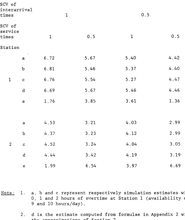
Table 3.3 Estimates of the Mean Number of Jobs SCV of interarrival times SCV of service times 1 0.5 1 0.5 0.5 1 Station a b 1 c d e a b 2 Note: c d e 1. 6.72 6.81 6.76 6.69 1.76 4.53 4.37 4.52 4.44 1.99 5.67 5.46 5.54 5.67 3.85 3.21 3.23 3.24 3.42 6.54 5.40 5.37 5.27 5.46 3.61 4.03 4.12 4.04 4.19 3.97 4.42 4.40 4.47 4.46 1.36 2.99 2.99 3.05 3.19 6.69
a, b and c represent respectively simulation estimates with 0, 1 and 2 hours of overtime at Station 1 (availability of 8, 9 and 10 hours/day).
2. d is the estimate computed from formulae in Appendix 2 with the approximations of Section 2.
3. e is the maximum % absolute error of d relative to estimates a, b, and c.
Table_ 3.4 Esiae of th ____ en ubr fJb ca cs STATION 1 1 1 2 3 1 1 0.5 2 3 1 0.5 1 2 3 1 0.5 0.5 2 3 Note: 1. a 4.55 6.83 4.48 3.67 5.18 3.17 3.50 5.81 4.14 2.89 4.54 3.04 b 4.41 6.65 4.40 3.73 5.15 3.18 3.55 5.91 4.14 2.91 4.56 3.02 c 4.37 6.73 4.46 3.76 5.23 3.19 3.61 5.82 4.11 2.88 4.43 3.00 d 4.44 6.69 4.44 3.74 5.17 3.32 3.58 6.23 4.35 2.89 4.74 3.24 e 2.42 2.05 0.91 1.91 1.15 4.73 2.29 7.23 5.84 0.69 7.00 8.00
ca and cs are the scv of the interarrival and service times respectively.
2. a, b and c are simulation estimates with availability of 8, 9 and 10 hours respectively at Station 2. At Stations 1 and 3 the availability is 8 hours.
3. d is the estimate computed from formulae in Appendix 2 with the approximation of Section 2.
4. e is the maximum % absolute error of d relative to estimates a, b and c.
III
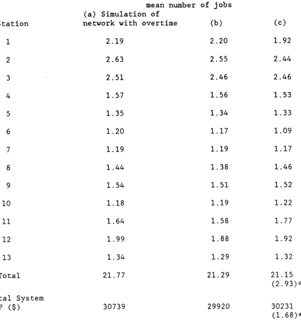
Table 3.5 Results of Tests with 10 Product. 13 Station Network
mean number (a) Simulation of
network with overtime 2.19 2.63 2.51 1.57 1.35 1.20 1.19 1.44 1.54 1.18 1.64 1.99 1.34 21.77 Total System WIP ($) 30739 of jobs (b) 2.20 2.55 2.46 1.56 1.34 1.17 1.19 1.38 1.51 1.19 1.58 1.88 1.29 21.29 29920 (c) 1.92 2.44 2.46 1.53 1.33 1.09 1.17 1.46 1.52 1.22 1.77 1.92 1.32 21.15 (2.93)* 30231 (1.68)**
Note: 1. a is the simulation estimate with the network data as specified in Appendix 3.
2. b is the simulation estimates with the network derived from approximations of Section 2.
3. c is the computed value for the network in b, with parametric decomposition approach (formulae in Appendix 2).
4. *maximum % error of approximation (c) relative to simulation values (a) and (b).
5. ** maximum % error in WIP value of (c) relative to simulation Station 1 2 3 4 5 6 7 8 9 10 11 12 13 Total
Appendix 1
Proof of Proposition 1:
First, we show that the proposition is true for job 1 and then, by induction, we show that it holds for any job i, i > 2. Recall that by notation (di -x, di + x) denotes an interval of length 2x hours, x
hours before and after departure of job i in System A. Note that, both A and Al are empty when job 1 arrives and the corresponding waiting times are zero. Also note that al:(dal, tal) al':(dal', tal'). We make the following observations about departure times d and dl':
(i) If the service time b is an integral number of days, i.e.,
bl = nl(r+ov) for some positive integer nl, then the corresponding
service time in Al is also equivalent to n days of work, i.e., bl' = nlr, and the departure instants d and d' are the same.
(ii) Let the service time for job 1 in A be equivalent to n days and n2 hours, i.e., b = nl(r+ov) + n2, where n is a non-negative
integer and 0 < n2 < (r+ov). Then the difference in the departure
times d and d' is entirely due to n2.
Let y = dal + L(bl + tal)/(r+ov)J,
1 (r - tal)/k, and z2 = tal + k(r - tal),
where LxJ denotes the largest integer not greater than x, Lx] denotes the smallest integer not smaller than x, and k is the scaling factor for process times as defined in Section 2.1. Observe that, depending on the value of n2, the completion of service for job 1 and its departure occur
either on day y or y+l in Systems A and Al.
We consider the following four mutually exclusive and collectively exhaustive cases to compare the departure times d and dl'. The reader
may find figure Al.1, which illustrates these cases, useful in understanding the arguments presented below.
Case (1): 0 < n2 (r - tal). Service is completed during regular time of day y in both A and Al. In this case,
ddl y, td1 tal + n2; ddl' - y and tdl' - tal + kn2.
Since td - td1' = (l-k)n2 n2 ov/(r+ov) r ov/(r+ov) k ov, we have Idl - dl'l k ov.
Case (2): r - ta1 < n2 z.1 In this case the service for job 1 is completed during overtime of day y (departure at the beginning of day y+l) in System A and during regular time of day y in Al.
ddl = y + 1, td1 0; ddl' y and td1' tal + kn2 By definition of zl and z2, z2 tdl' r.
Since r - z2 = (l-k) (r-tal) (l-k)r = ov r/(r+ov) = k ov, we have Idl - dl'l k ov.
Case (3): z1 < n2 (r + ov - tal). In this case service for job 1 is
completed during overtime of day y (and departure at the start of day y + 1) in A and during day (y+l) in Al.
dd1 = y + 1, td1 = 0; dd1 ' = y + 1 and td1' k(n2 - Zl)
The bounds on n2 imply that 0 td1' k ov and Idl - dl'j < k ov. Case (4): (r + ov - tal) < n2 < (r+ov). In this case the job is
completed during regular time of day y + 1 in both systems A and Al. ddl = y + 1, td1 = n2 - (r + ov- tal); ddl' = y + 1
and td1' = k(n2 - zl).
Note that tdl' - td1 = k(n2 - z1) n2 + (r + ov - tal) = ov[l - n2/(r + ov)].
Since n2 < (r + ov) , tdl' - td1 > 0, and
III
Hence dl - dl'J k ov and the proposition follows for job 1.
To prove the proposition for the general case, say job i, i 2, assume that the result is true for jobs 1, 2, ...i-l. To prove the proposition we consider four mutually exclusive and collectively exhaustive cases. Case (1): At time ai, the arrival epoch of job i, both A and Al are empty. This case is identical to that of job 1 and the result follows. Case (2): At time ai, A is busy and Al is idle.
Let j, j < i denote the last job before i which sees an idle server in System A upon arrival. (Clearly such a job exists.) Let sj and s'j denote the start time (day and hour) of service for job j in systems A and Al. Let si and s'i be the corresponding times for job i. We make
the following observations on the operation of A and Al. 1. sj = aj and s'j sj
2. The machine in A is busy from aj till the completion of service job i.
3. s'i = ai and si > s'i.
To derive the bounds on Idi - di'l, consider the following alternatives: (a) delay the start of service for job i in Al such that the start time is the same in both systems, i.e., it is si in both A and Al. Denote the departure time for job i in system Al so
modified as dl'
Clearly dl' > di'. By an analysis similar to that of job 1,
we obtain, di - k ov dl' di + k ov
which implies that di + k ov > di' (1)
(b) Consider a system Al in which the processing of job j starts at the same time as in A, i.e., s'j = sj and jobs j, j+l,... i are processed without any intervening idle time. Let d2'
denote the departure time of job i in system Al. It is clear that d2' < di'.
By treating jobs j through i as a single job with process time bj + bj+l + ... + bi, and an analysis similar to job 1, we obtain di - k ov d2'< di + k ov which implies that
di - k ov < di (2)
From (1) and (2), we have di - k ov < di' < di + k ov, and the
proposition follows.
Case (3): At time ai, A is idle and Al is busy.
This case can be analyzed in a manner similar to case (2). Let j denote the last job before i which sees an idle machine in Al upon arrival. Let sj and s'j (si and s'i) respectively denote the start of service for
job j (job i) in systems A and Al. Note that: 1. sj' = aj and sj > s'j
2. si = ai and s'i > i
3. System Al is busy from aj till the completion of service of job
i.
Consider the following alternatives:
(a) Delay the start of service for job i in A such that si = s'i.
Let dl denote the departure time of job i in A. Then dl > di, and di' - k ov < dl d'i + k ov which implies
di < di' + k ov (1)
(b) Consider a system A in which j starts at time aj and jobs j, j+l, ... i are processed without any intervening idle time.
Let d2 denote the departure time of job i. Then d2 < di, and di ' - k ov d2 < di' + k ov which implies that
From (1) and (2) di' - k ov < di < di ' + k ov and the proposition follows.
Case (4): At time ai both A and Al are busy.
In this case note that jobs i-1 and i are processed in sequence without any interruption. The completion of service for job i is determined by the time taken to process (bi1 + bi) in System A and k(bil.1 + bhi) in
system Al from the start of service for job i-1 in both systems.
Note that, by assumption Idi.1 - di-l'l k ov and this is independent of process time bi_1.
Replacing the process time of job i-l by (bi + bhi) and repeating the analysis for job i-1, we obtain di - d'il < k ov.
Proof of Proposition 2
Without any loss of generality we assume that
(i) If more than one machine is available, a job is assigned to the machine which became free first, and
(ii) The machines are numbered such that the first m jobs are respectively assigned to machines 1, 2, ...m1.
Lemma Al: Consider a system B in which all m machines work overtime, i.e., m2 ml1. suppose ml jobs with process times bl, b2, ... bm
are assigned to the m machines and begin service at the same time (say t = 0). Assume that in B also the jobs begin service at time t - 0. Then the order in which the m jobs complete service is the same in B and B1. And the sequence in which the machines become free is also identical in B and B1.
Lemma A2: In any given sample path defined by a sequence of job arrivals and associated service times, let
Jj(Jj') be the set of jobs assigned to the machine j, j - 1, 2, ...ml in system B(B1).
Then Jj - Jj' , j 1, 2, ... mi.
Outline of Proof of Proposition 2:
Observe that for any given sample path, B can be decomposed into ml single machine subsystems Aj for each machine j, j 1, 2, ...ml. Jobs in Jj represent the sequence of arrivals and associated service times for Aj.
Let Alj represent the approximation of section 2.1 for system Aj, and let d'j i represent departure times of job i in Alj, i e Jj, j
= 1, 2, ... ml.
From proposition 1, we have Idi - d'j i| < k ov, i c Jj, j = 1, 2,
... ml. (a)
Also observe that B can likewise be decomposed into m subsystems
Blj, j 1, 2, ... ml.
Furthermore, from Lemma A2 it follows that Blj and Alj are identical, i.e., both systems have same machine schedules, with identical job arrivals and service times.
Hence di' = d'j i, i Jj, j = 1, 2, ...ml (b) From (a) and (b), we obtain di - di' < k ov and the proposition
follows. Remark 1
Consider a multimachine system with m2 < ml. Assume that the job arrivals and service times are such that the number of jobs is at least ml in both systems B and B1 at any point in time. Also assume that at time t=O, the processing of first job is initiated in both systems B and B1. Let b* = Lbmax/bmin] where bmax and bmin
respectively denote maximum and minimum process times. Consider systems B and B1 at the start of any day, i.e., at any point in time T, where T is integral in number of days. Then, the number of jobs in the two systems do not differ by more than (ml - 1) (b* +
1) - 1.
Outline of Proof:
Since the number of jobs is at least ml in both B and B, the amount of work completed during the interval [O,T] are equivalent,
i.e., WP(T) = (mlr + m2ov)T, WP' (T) - mlrT, and WP' (T) = klWP(T), where WP(T) and WP' (T) respectively represent the amount of work processed in B and B during the interval O,T] and k is as defined in Section 2.2.
Let N(N') denote the set of jobs processed either completely or
partially in B(B1) during [O,T]. Let NC(NC') denoted the set of completed jobs in B(B1) and NP(NP') the set of in-process jobs. Let INCI = n and INC' = n'. Note that INPI IJNP' ml.
Let xj (xj'), j = 1, 2, ... ml be the amount of work completed on job in process on machine j in B(B1).
We make the following observations: ml1 (i) WP(T) = Z bi + Z xj iENC j-1 ml (ii) WP' (T) = Z bi' + Z xj' = kWP(T) iE NC' j=l
(iii) Since the priority discipline is FCFS, the start of service of job i implies that the number of completed jobs is i - m + 1.
CLAIM 1: n' > n - (ml - 1) (b* + 1) + 1
Case (b):
processed either partially or completely, only in B. A FCFS discipline implies that i > n + ml, and from observation (iii) above, it follows that n' i - ml + 1 > n + 1 > n
-(b* + )(m1 - 1) + 1.
N' N: Consider the schedule for processing jobs in the set N in system B with the following process times:
bl'i = klbi if i NC
= klxj if i NP and is being processed on machine j. Note that Z bl'i - WP'(T).
iEN
A job is considered in process, if it is assigned a machine and the service is not yet complete at the end of day T. We note that:
(i) At most m - 1 jobs are in-process.
(ii) At least one of the in-process jobs in B is also in-process in B. This is clearly true for job (n + ml) which is the last job to enter service.
(iii) At most m - 1 jobs in the set NP can be scheduled to start prior to those in NC.
(iv) If all jobs in the set NP start service only after the jobs in NC, then the number of completed jobs in B is at least n - ml + 1. (v) For each job j in NP that is scheduled to start before some jobs
in NC it is possible that amount of processing is greater than klxj. In that case, each such job can delay completion of at most
b* jobs.
(vi) (iii) and (iv) together imply that n' n - ml - b*(ml - 1) = n + 1 - (ml - )(b* + 1).
CLAIM 2: n > n' + 1 - (ml - l)(b* + 1). The arguments are similar to those in Claim 1. Claim 1 and 2 together imply that n - n'I <
(m1 - )(b* + 1) - 1.
Since job arrivals are identical in B and B, the above results implies that the number of jobs in the two systems do not differ by more than (ml - l)(b* + 1) - 1.
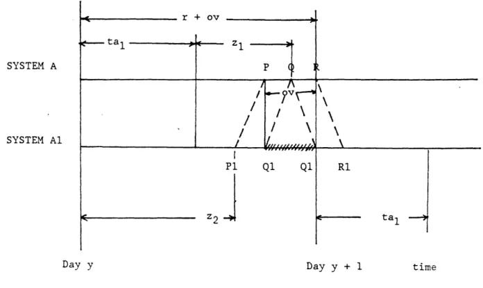
r + ov I - z1 P
/- ,
/1,
A
P1 Q1 Q1I---
Z2 J R1 tca l1Day y Day y + 1 time
denotes machine not available in Al (no overtime).
P and R represent start and completion of overtime in A.
P1 and R1 represent points in time in Al that correspond to P and R in A. (Corresponding points imply equivalent amount of work completion in
the two systems.)
Q1 is the corresponding point for Q in A and represents the start of day y+l and the end of day y.
FIGURE A.1 SYSTEM A
SYSTEM Al
e-
ta, --- :0Appendix 2
In this appendix, we present a summary of approximations based on the parametric decomposition approach for estimating mean number of jobs in open queueing networks with multiple products and deterministic routing. For details of these results, the reader is referred to Shanthikumar and Buzacott (1981), Whitt (1983, 1985) and Bitran and Tirupati (1988a). The approximations involve two steps: (a) determination of the mean and squared coefficient of variation (scv) of product flows in the network, and (b) estimation of the mean number of jobs in a GIIGIm queue.
Estimation of the mean and scv of product flows in the network:
Let m = number of products
J = number of stations
ai = arrival rate of product i
ui = number of operations required for product i ui,k = station visited by product i at step k
cdi,k = scv of product stream i after processing at step k (cdi,0 is the scv of product arrivals to the network.)
Aj = net arrival rate at station j
yj = service rate of each machine at station j caj = scv of arrivals at station j
cdj = scv of departures from station j csj = scv of service time at station j mj = number of machines at station j pj = utilization at station j = j/(mjpj)
m Ui
Aj = Z ailu i, r )' j 12, 2 J; (A2.1) i=1 r=l
cdj 1 + (1 - pj2) (caj - 1) + pj2(c pj + - 1) (A2.2)
m ui
ijca a icdir-lltUi r =
J)
j 1, 2, ...J (A2.3)i-l r=l
cdi,k Picdj + cni, k = 1, 2, .. .ui; i 1, 2, ...m (A2.4) where j = Ui,k, and Pi ai/Aj in (A2.4).
For the case where the arrival distribution of the aggregate product, i.e., the composition of all products arriving at station j except i, can be approximated by a Poisson distribution, (A2.4) reduces to
cdi,k Picdj + (l-pi){Pi+(l-Pi)cdik-l), k = 1, 2, ...ui (A2.4') i = 1, 2 ...m;
Other approximations for cni are discussed in Bitran and Tirupati
(1988a).
Estimation of mean number of jobs in a GIIGIm queue (see Whitt, 1985 for details)
Additional Notation:
Lqj = mean number of jobs in queue at station j Lj = mean number of jobs at station j
Lqj* = mean number of jobs in an MMIm queue with utilization pj.
Then Lj = Lqj + mjpj, (A2.5)
III
Case (1): m = 1:
Lqj = pj 2/(1-p) (caj + csj)/2 g(pj, caj, csj) (A2.6) 2
where g(p, ca, cs) = exp [-2(1-p)(1-ca) 2/(3p(ca + cs))], ca 1 = exp [-(l-p)(ca-l)/((l+p)(ca + 10cs2))], ca > 1 Case 2: m > 1:
Lqj = ,(pj, caj, sj, mj) caj + csj L(A2.7) 2
Where (p, ca, cs, m)
= 4 (ca - cs) 41 (m,p) + cs e ((ca + cs)/2,m,p), ca > cs
4 ca-3cs 4ca-3cs
= (cs-ca)/(2(ca+cs))3(m,p) + (cs+3ca)/(2(ca+cs))e((ca+cs)/2,m,p), cacs e(a,m,p) = 1 , a > 1 = (24(m,p)) 2 (1-a) o < < 1 6(m,p) = min (0.24, (l-p) (m-l) [ (4+5m)0 5 - 2]/(16mp)) 0l(m,p) = 1 + 6 (m,p) 02(m,p) = 1 - 4 6(m,p) 03(m,p) = 2(m,p) exp (-2(1-p)/(3p)) 04(m,p) = min (1, (l(m,p) + 3 (m,p) )/2 )
Appendix 3. Data for the Network Example (Section 3.3) Table A3.1: Product Data
Distribution of
Product interarrival Routing Sequence
times 1 Erlang, order 2 1,2,4,2,9,10,11 2 Erlang, order 2 1,2,5,2,8,9,10,11 3 Erlang, order 3 1,2,6,4,2,9,12,11 4 Erlang, order 3 1,2,7,4,2,9,10,11 5 Uniform 1,2,4,12,2,9,2,13 6 Erlang, order 3 1,2,5,12,2,9,7,13 7 Erlang, order 4 1,2,6,12,2,8,2,13 8 Exponential 1,2,3,7,4,12,2,8,6,9,2,13 9 Exponential 1,2,3,5,4,6,12,2,8,2,10,6,13 10 Erlang, order 3 1,2,3,6,2,4,12,7,2,9,11,5,13
Table A3.2: Station Data
Work
Service Time Schedule Utilization
Station Distribution vj hours/day (p-)
1 Erlang order 2 100 8.00 0.7692 2 Erlang order 4 1612 8.72 0.8284 3 Uniform 733 9.52 0.7979 4 Erlang order 2 1052 8.00 0.7000 5 Uniform 912 8.29 0.6861 6 Erlang order 4 1683 8.00 0.6501 7 Exponential 1662 9.20 0.5797 8 Erlang order 3 1812 10.13 0.7018 9 Erlang order 3 1730 8.96 0.7143 10 Erlang order 3 1600 8.56 0.6547 11 Uniform 1882 9.91 0.7418 12 Erlang order 2 1486 10.05 0.7495 13 Erlang order 2 3250 9.81 0.6522
Note: 1. The distribution of interarrival times for jobs in each product family is completely specified by data in Table A3.1
and the fact that the arrival rate is 1.0 per day.
2. The service time distribution at each station is completely specified by the data in Table A3.2 together with the net arrival rate computed from routing data (using formulae in Appendix 2) in Table A3.1.
M.I.T.Sloan School of Management Working Paper Series
Papers by Gabriel R. Bitran
Nippon Telegraph and Telephone Professor of Management Science
Paper # Date TitlelAuthor(s)
3115 1/90 "Analysis of Phi / PH / 1 Queues," Bitran, G.R., and Dasu, S. 3111 1/90 "Distribution-Free, Uniformly-Tighter Linear Approximations for
Chance-Constrained Programming," Bitran, G., and Leong, T. 3108 12/89 "Hotel Sales and Reservations Planning," Bitran, G., and Leong, T. 3097 11/89 "Co-Production of Substitutable Products," Bitran, G., and Leong,
T.Y.
3090 11/89 "Ordering Policies in an Environment of Stochastic Yields and Substitutable Demands," Bitran, G., Dasu, S.
3071 8/89 "Deterministic Approximations to Co-Production Problems with Service Constraints" Bitran, G., and Leong, T.
3054 "Sequencing Production on Parallel Machines with Two Magnitudes of Sequence Dependent Setup Costs," Bitran, G., and Gilbert, S. 3019 "Ordering Policies in an Environmnent of Stochastic Yields and
Substitutable Demands," Bitran, G., and Dasu, S.
3017 "Hierarchical Production Planning," Bitran, G., and Tirupati, D. 2519 3/89 "Approximation for Manufacturing Networks of Queues and
Overtime," Bitran, G., and Tirupati, D.
1744 2/86 "Planning and Scheduling for Epitaxial Wafer Production Facilities," Bitran, G., and Tirupati, D.
1764 3/86 "Multiproduct Queueing Networks with Deterministic Routing: Decomposition Approach and the Notion of Interference," Bitran, G., and Tirupati, D.
1635 3/85 "An Optimization Approach to the Kanban System," Bitran, G., and Chang, L.
1486 10/83 "Introduction to Multi-Plant MRP," Bitran, G., Marieni, D., and Noonan, J.
1402 2/83 "A Simulation Model for Job Shop Scheduling," Bitran, G., Dada, M., and Sison, L.
1391 1/83 "Productivity Measurement at the Micro Level," Bitran, G., and Chang, L.
Ill
Paper # Date Title/Author(s)
1282 2/82 "Analysis of the Uncapacitated Dynamic Lot Size Problem," Bitran, G.R., Magnanti, T.L., and Yanasse, H.H.
1271 11/81 "Computational Complexity of the Capacitated Lot Size Problem," Bitran, G.R., and Yanasse, H.H.
1272 10/81 "Diagnostic Analysis of Inventory Systems: A Statistical Approach," Bitran, G.R., Hax, A.C., and Valor-Sabatier, J.