Experimental study of underexpanded round jets : nozzle lip thickness effects and screech closure mechanisms investigation

Pour l'obtention du grade de

DOCTEUR DE L'UNIVERSITÉ DE POITIERS École nationale supérieure d'ingénieurs (Poitiers)

Pôle poitevin de recherche pour l'ingénieur en mécanique, matériaux et énergétique - PPRIMME (Poitiers) (Diplôme National - Arrêté du 25 mai 2016)

École doctorale : Sciences et ingénierie en matériaux, mécanique, énergétique et aéronautique -SIMMEA (Poitiers)

Secteur de recherche : Mécanique des milieux fluides et acoustique

Présentée par :

Thiago Lima De Assuncao

Experimental study of underexpanded round jets :

nozzle lip thickness effects and screech closure

mechanisms investigation

Directeur(s) de Thèse : Yves Gervais, Stève Girard

Soutenue le 20 décembre 2018 devant le jury

Jury :

Président Eric Goncalves Professeur, ISAE, ENSMA, Poitiers

Rapporteur Stéphane Barre Directeur de recherche, LEGI, CNRS, Grenoble Rapporteur Estelle Piot Ingénieure de recherche, ONERA, Toulouse Membre Yves Gervais Professeur, PPRIME, Université de Poitiers

Membre Peter Jordan Chargé de recherche, PPRIME, ENSIP, Université de Poitiers Membre Christophe Schram Professeur, Institut Von Karman, Bruxelles, Belgique

Membre Daniel Edgington-Mitchell Professor, Monash University, Melbourne, Australia Membre Vincent Jaunet Maître de conférences, ISAE, ENSMA, Poitiers

Pour citer cette thèse :

Thiago Lima De Assuncao. Experimental study of underexpanded round jets : nozzle lip thickness effects and

screech closure mechanisms investigation [En ligne]. Thèse Mécanique des milieux fluides et acoustique. Poitiers :

_____________________________________________________________________________

THÈSE

Pour l’obtention du Grade de

DOCTEUR DE L’UNIVERSITÉ DE POITIERS

&

FACULTÉ DES SCIENCES FONDAMENTALES ET APPLIQUÉES

(Diplôme National - Arrêté du 7 août 2006)

École Doctorale

: Sciences et Ingénierie en Matériaux, Mécanique, Energétique et

Aéronautique.

Spécialité :

MÉCANIQUE DES MILIEUX FLUIDES ET ACOUSTIQUE

Présentée par

Thiago Lima de Assunção

Experimental Study of Underexpanded Round Jets: Nozzle Lip

Thickness Effects and Screech Closure Mechanisms Investigation

Directeur de thèse : Yves Gervais

Co-direction : Vincent Jaunet & Stève Girard

Soutenue le 20 12 2018

Devant la Commission d’Examen

JURY

Estelle PIOT

Ingénieure de Recherche, ONERA, France

Rapporteur

Stéphane BARRE

Directeur de Recherche, CNRS, France

Rapporteur

Christophe SCHRAM

Professeur, VKI, Belgium

Examinateur

Daniel

EDGINGTON-MITCHELL

Professeur, Monash University, Australia

Examinateur

Éric GONCALVES

Professeur, ISAE-ENSMA, France

Examinateur

Peter JORDAN

Chargé de Recherche, CNRS, France

Examinateur

Yves GERVAIS

Professeur, Université de Poitiers, France

Examinateur

Vincent JAUNET

Maitre de Conférence, ENSMA, France

Examinateur

ACKNOWLEDGEMENTS

I would like to express my eternal gratitude to my advisor, Prof. Yves Gervais and co-advisors, Dr. Stève Girard and Dr. Vincent Jaunet. Prof. Yves always encouraged me in this very important task, giving me academic support to reach my research objectives. I am also extremely grateful to Dr. Stève for his meaningful help with the laboratory facilities and attention spent from the time of my arrival in Poitiers, providing me with the necessary serenity to carry out my work. I thank Dr. Vincent Jaunet for his crucial contribution in this work, providing enthusiastic discussions and meaningful advice about the Screech phenomenon research.

Special thanks to Dr. Matteo Mancinelli for his meaningful discussion on the VS model and Dr. Guillaume Lehnasch and Dr. Anton Lebedev for their constructive criticism of the work. I would also like to express thanks to the jury members: Dr.

Estelle Piot,

I extend my sincere gratitue to my dear colleagues from the “salle des doctorants” (Igor, Selène, Marc, Tamon, Oghuzan, Maxime, Filipe, Eduardo and Ugur) for creating an awesome atmosphere of work and comradery.

I could not forget to express my thanks to all of the staff at the Prime Institut (Alex, Thomas, Romain T., Romain B., Damien, Redouane, Patrick B., Patrick L., Dominique and Nicolas) for their technical contribution in this work. Moreover, special thanks to Mme. Nadia Maamar for her important administrative support throughout the whole of my stay in France.

Thanks to the Brazilian National Council for Scientific and Technological Development (CNPq) for their support with tuition fees and the Brazilian Air Force (FAB) for the opportunity and financial resources.

Finally, I would like to express my infinite gratitude to my parents (Severino and Mônica) for their endless love. To end, I am immeasurably grateful to my beloved wife, Cintia, for her unconditional love and support, which has given me two blessed children: Matheus and Marina.

RESUME

Cette thèse est une contribution expérimentale à l’étude des résonances aéroacoustiques des jets sous-détendus : le Screech. Diverses méthodes expérimentales sont utilisées à cette fin, telles que la mesure de pression acoustique, la strioscopie et la Vélocimétrie par Image de Particules, et associées à des techniques classiques de post-traitement comme les décompositions en mode de Fourier et aux valeurs propres. Ces Techniques permettent d’évaluer les effets d’épaisseur de la lèvre de la buse sur l’écoulement, et fournissent des informations sur les différences de comportement d’un même jet montrant des modes oscillatoires différents. Enfin, on entreprend d’étudier la présence de divers mécanismes de fermeture de la boucle de résonance pour divers modes de Screech. La présence d’ondes intrinsèques au jet, se propageant vers l’aval pour les modes axisymétrique (A2) et hélicoïdal (C) suggèrent que ces ondes puissent jouer un rôle dans la résonance. La signature de ces ondes n’est en revanche pas attestée pour les modes battants (B). Ces résultats semblent donc indiquer que plusieurs mécanismes de rétroaction différents puissent être à l’oeuvre dans la résonance du jet sous-détendu.

ABSTRACT

This work provides an experimental contribution to the study of the Screech phenomenon. Various experimental techniques such as microphones array, Schlieren and Particle Image Velocimetry (PIV) together with advanced post-processing techniques like azimuthal Fourier decomposition and Proper Orthogonal Decomposition (POD) are employed. These techniques enable the evaluation of the lip thickness effects on the jets generated by two different round nozzles. The differences on the flow aerodynamics and acoustics are discussed. Then, we carry out experiments to analyse the effects of the different dominant Screech modes (B and C) on the flow characteristics. No noticeable differences are found in the mean fields. However, the fluctuation fields shows the contrary: B mode has larger fluctuation. In the last part, we investigate the Screech closure mechanism. The signature of upstream jet waves is revealed in the axisymmetric (A2) and helical (C) mode. However, the mode B does not present evidence of this instability in the flow, indicating that its closure mechanism may be bonded to another kind of waves. The conclusion from these results is that the Screech phenomenon seems be driven by different closure mechanisms.

TABLE OF CONTENTS

ACKNOWLEDGEMENTS ... ii

RESUME ... iii

ABSTRACT ...iv

LIST OF FIGURES ... viii

INTRODUCTION ... 1 1 PHENOMENOLOGY ... 3 1.1 Underexpanded Jets ... 3 1.1.1 Compressibility Effects ... 5 1.1.2 Turbulence ... 7 1.1.3 Shock-Cell Structure ... 9 1.1.3.1 Shock Leakage ... 11 1.1.3.2 Shock Oscillations ... 12 1.2 Screech ... 14

1.2.1 Underexpanded Jet Noise in Convergent Nozzle ... 14

1.2.2 Screech Modes and Staging ... 15

1.2.3 Mechanism ... 17

1.2.4 Sources and Directionality ... 20

1.2.5 Jet Temperature Influence ... 21

1.2.6 Nozzle Lip Thickness Influence ... 22

1.2.7 Cessation ... 23

1.2.8 Frequency Estimation ... 23

1.2.9 Screech Influence on Jet Topology ... 28

1.3 Conclusion ... 28

2 EXPERIMENTAL TECHNIQUES AND FACILITIES ... 29

2.1 Supersonic Flow Facility ... 29

2.2 Acoustic Measurements ... 30

2.3 Schlieren Experiments ... 31

2.4 PIV Experiments ... 32

2.5 POD analysis ... 36

3 NOZZLE LIP THICKNESS EFFECTS ... 39

3.1.1 Far-Field Screech Noise ... 39

3.1.2 Relation Between Screech and Azimuthal Fourier Modes ... 41

3.1.3 Conclusion ... 43

3.2 Flow Topology ... 44

3.2.1 Average Flow Topology and Shock-Cell Spacing ... 44

3.2.2 Standing Wavelength ... 45

3.2.3 Mean Velocity Fields ... 47

3.2.4 Velocity Fluctuation Fields ... 50

3.2.4.1 Turbulence Intensity ... 52 3.2.4.2 Reynolds Stress ... 55 3.2.4.3 Compressibility Effects ... 56 3.2.5 Conclusion ... 59 3.3 Flow Structures ... 60 3.3.1 Hydrodynamic wavelength (Lh) ... 60 3.3.2 Structures Dynamics... 61 3.3.3 Conclusion ... 66

4 SCREECH MODES EFFECTS ... 67

4.1 Flow Topology ... 67

4.1.1 Average Flow Topology and Shock-Cell Spacing ... 67

4.1.2 Standing Wavelength ... 67

4.1.3 Mean Velocity Fields ... 68

4.1.4 Velocity Fluctuations Fields ... 70

4.1.4.1 Turbulence Intensity ... 71

4.1.4.2 Reynolds Stress and Anisotropy ... 72

4.1.5 Conclusion ... 73

4.2 Flow Structures ... 74

4.2.1 Hydrodynamic wavelength (Lh) ... 74

4.2.2 Structures Dynamics... 74

4.2.3 Conclusion ... 76

5 CLOSURE MECHANISMS INVESTIGATION ... 79

5.1 Upstream Neutral Waves Theory ... 79

5.2 Upstream Neutral Jet Waves and Screech Modes ... 84

5.3 Signature of Upstream Neutral Waves in the Flow... 86

5.3.2 Axisymmetric Screech Mode (A2) ... 87

5.3.3 Helical Screech Mode (C) ... 92

5.3.4 Flapping Screech Mode (B) ... 96

5.4 Screech Staging ... 100

5.5 Conclusion ... 101

6 CONCLUDING REMARKS AND PERSPECTIVES ... 102

LIST OF FIGURES

Figure I. 1: a) skin and b) stringer cracks. Hay & Rose (1970). ... 2

Figure 1. 1: three kinds of jet topology as a function of exit conditions. Overexpanded on the top, perfectly expanded in the middle and underexpanded at the bottom. Anderson Jr (1991). 4 Figure 1. 2: global jet structure. Lehnasch (2005). ... 4

Figure 1. 3: sketch of the jet mixing layer. U1 and U2 are the fast and slow flow velocities in each side of the mixing layer, and Uc is the velocity of instabilities. ... 5

Figure 1. 4: experimental data of compressible mixing layer growth rate, normalized by incompressible value. Papamoschou & Roshko (1988). ... 7

Figure 1. 5: Kelvin-Helmholtz instabilities. Brown & Roshko (1974). ... 7

Figure 1. 6: shock-cell structure scheme. Savarese (2014). ... 9

Figure 1. 7: Schlieren visualisation of shock-cell structure of the underexanded jet at Mj=1.50. ... 10

Figure 1. 8: Schlieren visualisation of a jet at Mj=1.61 with a marked Mach disk. ... 10

Figure 1. 9: instantaneous snapshots of shock leakage dynamic. Daviller et al. (2013). ... 12

Figure 1. 10: phase-average PMT data obtained at nine radial positions, on third shock in Mj=1.42 and at the different phases of Screech cycle (τ/Ts). Panda (1998). ... 13

Figure 1. 11: PSD (Power Spectral Density) of near-field microphone signal (gray) and PSDx105 of the signal of containing the axial location at the first shock tip at NPR 2.27 (black). André et al. (2011). ... 14

Figure 1. 12: noise intensity for nozzles undergoing different operating conditions. Tam & Tanna (1982). ... 14

Figure 1. 13: typical jet noise spectrum of underexpanded nozzle in far field at Mj=1.35. The black line represents mixing noise, red line the broadband noise, blue line the screech noise and green line is the combination between mixing and broadband noise. André (2012). ... 15

Figure 1. 14: screech modes for a circular convergent nozzle. Panda et al. (1997). ... 15

Figure 1. 15: fundamental Screech frequency versus Mj for 37.6 mm circular convergent nozzle. Clem et al. (2012) ... 16

Figure 1. 16: screech frequency versus NPR. Frequencies of dominant modes (circles) and secondary modes (crosses). Powell et al. (1992). ... 17

Figure 1. 17: diagram of screech loop (solid lines) and associated phenomena (dashed lines). Raman (1999). ... 18

Figure 1. 18: Schlieren image of rectangular nozzle operating in screech loop. Mj = 1.5. Raman (1997). ... 18

Figure 1. 19: sketch of the first Screech closure mechanism (classical model). ... 19

Figure 1. 20: sketch of the second Screech closure mechanism (jet modes). ... 19

Figure 1. 21: Screech intensity directionality. Powell (1953a). ... 21

Figure 1. 22: dependence of the Screech modes with temperature for several Mj conditions, a) unheated jets and b) temperature ratio (Tr) 2.78. Massey & Ahuja (1997). ... 21

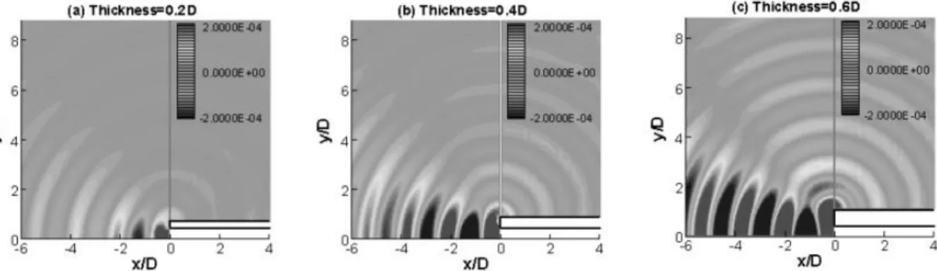
Figure 1. 23: comparison of instantaneous scattered pressure fields. Nozzle lip thickness: a) 0.2D, b) 0.4 D and c) 0.6D. Kim & Lee (2007). ... 22

Figure 1. 24: shifting of rectangular jet Screech cessation versus Mj for various lip thickness.

Raman (1997). ... 23

Figure 1. 25: a) amplitudes of the pressure fluctuations in the near field and b) steamwise velocity of screeching jets at Mj= 1.30. The vertical arrows in the figures represent shock locations. Gao & Li (2009). ... 26

Figure 1. 26: average shock-cell and standing wave spacing versus Mj for 3 nozzle geometries: a) circular, b) rectangular and c) elliptical. Panda et al. (1997). ... 27

Figure 2. 1: evaluated nozzles. Thin lip (left) and thick lip (right). ... 29

Figure 2. 2: coordinates system centered at the nozzle exit (top) and layout of supersonic flow facility (bottom)... 30

Figure 2. 3: microphone array employed for azimuthal Fourier decomposition. ... 30

Figure 2. 4: Toepler Z-type Schlieren layout. Settles & Hargather (2017), modified. ... 32

Figure 2. 5: PIV system ... 33

Figure 2. 6: statistic convergence of the PIV data. Mj=1.5 thick lip B mode. ... 34

Figure 2. 7: ratio between number of the spurious vectors and total sample size. Mj=1.5, thick lip dominant flapping mode B. ... 35

Figure 2. 8: longitudinal mean velocity (U) normalized by Ue for Mj=1.13. GPU (left) and CPU processing (right)... 36

Figure 2. 9: particle effect in the noise spectrum for Mj=1.13, thin (left) and thick (right) lip nozzle. ... 36

Figure 3. 1: cartography of the PSD of far-field noise of the screeching jets generated by thin (top) and thick (botton) lip nozzle. ... 40

Figure 3. 2: comparison between far-field pressure spectrum generated by two different nozzles: thick lip (magenta) and thin one (green). ... 41

Figure 3. 3: cartography of the PSD of the first azimuthal mode (m=0) of the near-field pressure as a function of St number and Mj. Effect of the nozzle lip on A1/A2 Screech modes: thin (top) and thick lip (bottom). ... 42

Figure 3. 4: cartography of the PSD of the first azimuthal mode (m=1) of the near-field pressure as a function of St number and Mj. Effect of the nozzle lip on B/C/D Screech modes: thin (top) and thick lip (bottom). ... 43

Figure 3. 5: mean density gradient fields for Mj= 1.5, thin (left) and thick lip (right). Shock-cell length represented in axial coordinate. ... 44

Figure 3. 6: average shock-cell spacing. Comparison between theory and experimental data . 45 Figure 3. 7: rms of grey level fluctuations of the jet at Mj=1.33. Thin (left) and thick lip (right) nozzles. ... 46

Figure 3. 8: longitudinal rms velocity fluctuation (u’rms) normalized by Ue and standing waves (SW) identification. Jet at Mj = 1.33 generated by the thick lip nozzle. ... 46

Figure 3. 9: comparison of the standing wavelength for the thin and thick nozzle ... 47

Figure 3. 10: longitudinal mean velocity (U) normalized by Ue for Mj=1.33. Thin (left) and thick (right) lip nozzles. ... 48

Figure 3. 11: longitudinal mean velocity (U) normalized by Ue for Mj = 1.5. Thin (left) and thick (right) lip nozzles. ... 48

Figure 3. 12: longitudinal mean velocity (U) normalized by Ue for Mj = 1.61. Thin (left) and thick

(right) lip nozzles. ... 48

Figure 3. 13: mean axial velocity profile normalized by Ue for Mj=1.33. ... 49

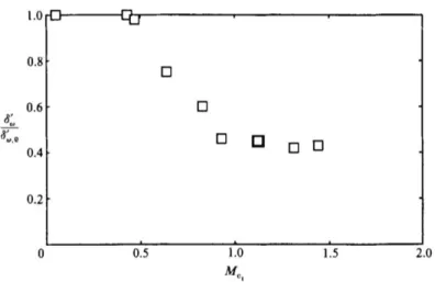
Figure 3. 14: mixing layer vorticity thickness evolution Mj = 1.33, thin and thick lip nozzle. ... 49

Figure 3. 15: spreading rate for all Mj conditions considered. ... 50

Figure 3. 16: longitudinal rms velocity fluctuation (u’rms) normalized by Ue for Mj=1.33. Thin (left) and thick (right) lip nozzles. ... 51

Figure 3. 17: longitudinal rms velocity fluctuation (u’rms) normalized by Ue for Mj = 1.5. Thin (left) and thick (right) lip nozzles. ... 51

Figure 3. 18: longitudinal rms velocity fluctuation (u’rms) normalized by Ue for Mj=1.61. Thin (left) and thick (right) lip nozzles. ... 51

Figure 3. 19: transversal rms velocity fluctuation (v’rms) normalized by Ue for Mj = 1.33. Thin (left) and thick (right) lip nozzles. ... 52

Figure 3. 20: transversal rms velocity fluctuation (v’rms) normalized by Ue for Mj =1.5. Thin (left) and thick (right) lip nozzles. ... 52

Figure 3. 21: transversal rms velocity fluctuation (v’rms) normalized by Ue for Mj=1.61. Thin (left) and thick (right) lip nozzles. ... 52

Figure 3. 22: maximum longitudinal turbulence intensity for Mj=1.13. ... 53

Figure 3. 23: maximum longitudinal turbulence intensity for Mj=1.33. ... 53

Figure 3. 24: maximum longitudinal turbulence intensity for Mj=1.5. ... 53

Figure 3. 25: maximum transversal turbulence intensity for Mj = 1.13 ... 54

Figure 3. 26: maximum transversal turbulence intensity for Mj=1.33. ... 55

Figure 3. 27: maximum transversal turbulence intensity for Mj=1.5. ... 55

Figure 3. 28: maximum Reynolds stress in the mixing layer for Mj =1.13 ... 56

Figure 3. 29: maximum Reynolds stress in the mixing layer for Mj=1.33. ... 56

Figure 3. 30: maximum Reynolds stress in the mixing layer for Mj=1.5. ... 56

Figure 3. 31: maximum longitudinal turbulence vs shock-cell length for all Mj analysed conditions. Thick lip nozzle. ... 57

Figure 3. 32: maximum longitudinal turbulence vs shock cell length for all Mj analysed conditions. Thin lip nozzle. ... 57

Figure 3. 33: maximum transversal turbulence vs shock cell length for all Mj analysed conditions. Thick lip nozzle. ... 58

Figure 3. 34: maximum transversal turbulence vs shock cell length for all Mj analysed conditions. Thin lip nozzle. ... 58

Figure 3. 35: maximum Reynolds stress vs shock cell length for all Mj analysed conditions. Thick lip nozzle. ... 59

Figure 3. 36: maximum Reynolds stress vs shock cell length for all Mj analysed conditions. Thin lip nozzle. ... 59

Figure 3. 37: correlation coefficient (R) for the jet at Mj=1.5 generated by thick lip nozzle. The reference points are represented by intersecting dashed lines: shock line (left) and standing wave (right). ... 60

Figure 3. 38: correlation coefficient (R) for the jet at Mj=1.33. The reference point is located inside the standing waves and is represented by the intersecting dashed lines. Thin (left) and thick (right) lip nozzle. ... 61

Figure 3. 39: correlation coefficient (R) for the jet at Mj=1.5. The reference point is located inside the standing waves and is represented by the intersecting dashed lines. Thin (left) and

thick (right) lip nozzle. ... 61

Figure 3. 40: transverse spatial (φ1 and φ2) POD modes for Mj =1.13, thin lip nozzle. ... 62

Figure 3. 41: transverse spatial (φ1 and φ2) POD modes for Mj=1.13, thick lip nozzle. ... 63

Figure 3. 42: streamwise spatial (φ1 and φ2) POD modes for Mj =1.5, thin lip nozzle. ... 63

Figure 3. 43: streamwise spatial (φ1 and φ2) POD modes for Mj =1.5, thick lip nozzle. ... 63

Figure 3. 44: phase portrait of the temporal coefficients a1 and a2 (left). Relative POD modes energy (right) for Mj =1.13, thick lip nozzle. ... 64

Figure 3. 45: phase portrait of the temporal coefficients a1 and a2 (left). Relative POD modes energy (right) for Mj=1.13, thin lip nozzle. ... 65

Figure 3. 46: phase portrait of the temporal coefficients a1 and a2 (left). Relative POD modes energy (right) for Mj=1.5, thick lip nozzle. ... 65

Figure 3. 47: phase portrait of the temporal coefficients a1 and a2 (left). Relative POD modes energy (right) for Mj= 1.5, thin lip nozzle... 66

Figure 4. 1: mean density gradient for Mj = 1.5. Flapping (left) and helical (right) Screech modes. Shock-cell spacing represented in axial coordinate. ... 67

Figure 4. 2: rms intensity of grey level fluctuations. B flapping (left) and C helical modes (right). ... 68

Figure 4. 3: longitudinal mean velocity (U) normalized by Ue. Flapping (left) and helical (right) Screech modes. ... 68

Figure 4. 4: transversal mean velocity (V) normalized by Ue. Flapping (left) and helical (right) Screech modes. ... 69

Figure 4. 5: mean axial velocity profile, normalized by Ue, for the jet at Mj=1.5. ... 69

Figure 4. 6: mixing layer velocity profiles. ... 70

Figure 4. 7: mixing layer thickness evolution. Flapping (red) and helical Screech mode (blue). 70 Figure 4. 8: longitudinal rms velocity fluctuation (u’rms) normalized by Ue. Flapping (left) and helical (right) Screech mode... 71

Figure 4. 9: transversal rms velocity fluctuation (v’rms) normalized by Ue. Flapping (left) and helical (right) Screech mode... 71

Figure 4. 10: maximum longitudinal turbulence intensity. Flapping (red) and helical Screech mode (blue). The shock positions are represented by dashed lines from Prandt-Pack’s theory. ... 72

Figure 4. 11: maximum transversal turbulence intensity. Flapping (red) and helical Screech mode (blue). The shock positions are represented by dashed lines from Prandt-Pack’s theory. ... 72

Figure 4. 12: maximum Reynolds stress in the mixing layer. Flapping (red) and helical (blue) modes. Shock positions represented by dashed lines from Prandt-Pack’s theory. ... 73

Figure 4. 13: maximum Anisotropy in the mixing layer. Flapping (red) and helical (blue) modes. Shock positions represented by dashed lines from Prandt-Pack’s theory. ... 73

Figure 4. 14: correlation coefficient (R). The reference point is placed in the standing waves and represented by intersecting dashed lines. Jet under dominant flapping B (left) and helical C (right) Screech mode. ... 74

Figure 4. 16: streamwise spatial (φ1 and φ 2) POD modes for C mode. ... 75

Figure 4. 17: phase portrait of the temporal coefficients a1 and a2 (left). Relative POD modes energy (right) for the flapping B Screech mode. ... 76 Figure 4. 18: phase portrait of the temporal coefficients a1 and a2 (left). Relative POD modes energy (right) for the helical C Screech mode. ... 76

Figure 5. 1: pressure eigenfunction of upstream subsonic waves. Cold jets, Mach number 1.5. a) (0,1) mode, κRj=0.7, b) (0,3) mode, κRj=3.0, and c) (0,5) mode, κRj=5.5. Tam & Hu (1989). 80 Figure 5. 2: sketch of cylindrical vortex-sheet. Tam & Hu (1989) modified. ... 80 Figure 5. 3: Left: dispersion relations of axisymmetric jet neutral modes for Mj =1.5 and

Temperature ratio (T) equals to 1. Dashed line represents the sonic condition (κ=-ω/a0), S and

B represent the saddle and branch points, respectively. Right: allowable frequencies of upstream neutral waves (m,n=0,2). Green dashed line represents the upper frequency limit (saddle point) and black dashed line represents the bottom frequency limit (branch point). Taken from Mancinelli (2018), internal report. ... 83 Figure 5. 4: sketch of Kelvin-Helmholtz (KH) and upstream travelling neutral waves (κ-). ... 84 Figure 5. 5: allowable frequency ranges for axisymetric (m=0,n=2) upstream-travelling jet neutral waves overlaped on the PSD of the acoustic pressure cartography of the axisymmetric azimuthal Fourier mode. Thick (left) and thin (right) lip nozzle. Solid and dashed lines

represent saddle and branch points, respectively. ... 85 Figure 5. 6: allowable frequency ranges for helical (m=1,n=1) upstream-travelling jet neutral waves overlaped on the PSD of the acoustic pressure cartography of the azimuthal Fourier mode 1. Thick (left) and thin (right) lip nozzle. Solid and dashed lines represent saddle and branch points, respectively. ... 85 Figure 5. 7: spatial POD functions (Φ) of the modes 1 and 2, for the streamwise (top) and transverse (bottom) velocity components. Each mode is individually normalized by its

respective maximum value of Φ . ... 88 Figure 5. 8: temporal coefficients a1a2 (left) and relative modes energy (right) for Mj=1.13, A2

mode, thick lip nozzle. ... 88 Figure 5. 9: wavenumber spectrum of the coherent streamwise velocity (𝑢𝑘𝑐). Vertical dashed lines represent the wavenumbers associated to the speed of sound at the Screech frequency in the upstream (negative values) and downstream (positive values) directions. ... 89 Figure 5. 10: amplitude of the downstream travelling waves normalized by the maximum value. ... 89 Figure 5. 11: amplitude of the upstream-travelling waves component associated to the

negative wavenumbers (kDj=-5.45 and -7.25), normalized by the overall maximum value. ... 90

Figure 5. 12: amplitude of the upstream-travelling waves component associated to the negative wavenumbers (k-), normalized by the maximum value of 𝑢𝑑𝑐. Mj =1.09 left and 1.14

right. Edgington-Mitchell et al. (2018). ... 90 Figure 5. 13: solutions of the cylindrical vortex-sheet dispersion relation. Chosen point (green) in the family of waves (m=0,n=2). ... 91 Figure 5. 14: Comparison between the amplitude of the velocity at the axial position x/D=1.0 of the experimental upstream-travelling waves and the theoretical vortex-sheet eigenfunction for (m=0, n=2). Mj=1.13, the velocities are normalized by their value at the jet axis (r/D=0). .. 91

Figure 5. 15: spatial POD functions (Φ) of the modes 1 and 2, for the streamwise (top) and transverse (bottom) velocity components. Each mode is individually normalized by the

respective maximum value of Φ . ... 92 Figure 5. 16: temporal coefficients a1a2 (left) and relative modes energy (right) for Mj=1.5, C

mode, thick lip nozzle. ... 93 Figure 5. 17: wavenumber spectrum of the coherent streamwise velocity (𝑢𝑘𝑐). Vertical

dashed lines represent the wavenumbers associated to the speed of sound at the Screech frequency in the upstream (negative values) and downstream (positive values) directions. .... 93 Figure 5. 18: amplitude of the downstream travelling waves normalized by the maximum value. ... 94 Figure 5. 19: amplitude of the upstream-travelling waves component associated to the

negative wavenumbers (kDj=-2.92 and -4.1), normalized by the overall maximum value... 94

Figure 5. 20: solutions of the cylindrical vortex-sheet dispersion relation. Chosen point (green) in the family of waves of κ (m=1,n=1). ... 95 Figure 5. 21: Comparison between the amplitude of the velocity at the axial position x/D=5.0 of the experimental upstream-travelling waves and the theoretical vortex-sheet eigenfunction for

k(m=1,n=1), Mj=1.5. The velocities are normalized by the maximum value inside of the jet. ... 95

Figure 5. 22: spatial POD functions (Φ) of the modes 1 and 2, for the streamwise (top) and transverse (bottom) velocity components. Each mode is individually normalized by the

respective maximum value of Φ . ... 96 Figure 5. 23: temporal coefficients a1a2 (left) and relative modes energy (right) for Mj=1.5, B

mode, thick lip nozzle. ... 97 Figure 5. 24: wavenumber spectrum of the coherent streamwise velocity (𝑢𝑘𝑐). Vertical

dashed lines represent the wavenumbers associated to the speed of sound at the Screech frequency in the upstream (negative values) and downstream (positive values) directions. .... 97 Figure 5. 25: amplitude of the downstream travelling waves normalized by the maximum value. ... 98 Figure 5. 26: amplitude of the upstream-travelling waves component associated to the

negative wavenumbers (kDj=-3.4 and -5.1), normalized by the maximum value. ... 98

Figure 5. 27: solutions of the cylindrical vortex-sheet dispersion relation. Chosen points: green at the region of κ (m=1,n=1) and blue at the region of κ (m=1,n=2). ... 99 Figure 5. 28: Comparison between the amplitude of the velocity at the axial position x/D=3.0 of the experimental upstream-travelling waves and theorical vortex-sheet eigenfunction for

k(m=1,n=1). Mj=1.5, flapping mode (B), the velocities are normalized by the maximum value

inside of the jet. ... 99 Figure 5. 29: sketch of the Screech phenomenon. ... 100

INTRODUCTION

The aircraft noise at take off and landing is a well remarked social problem due to the settlements surrounding airports as well as the increase in air traffic. Hence, the society has demanded solutions to improve acoustic comfort either by political petition or by mobilization of public opinion. One recent example of this protest could be observed in the discussion about the airport project in the region of Notre-Dame-des-Landes, France. Aware of the importance of the subject, the stakeholders of the air transport have attempted to decrease the levels of the aircraft noise. For instance, in France, it is possible to mention the IROQUA (Initiative de Recherche pour l’Optimisation Acoustique Aeronautique) that was created in 2005 and established a collaborative network composed by research institutes (CNRS and ONERA) and enterprises (Safran, Airbus and Dassault Aviation) with the purpose of developing research that aims to decrease the noise generated by aircrafts, including the jet noise which is composed by mixing noise, BBSAN and Screech. Similar initiative has been developed in Brazil, in the scope of the Projeto Silence, with participation of UFSC (Universidade Federal de Santa Catarina) and Embraer.

The expansion process of underexpanded sonic jets in quiescent atmosphere leads to the formation of a train of shock-cell structures within the potential core, interacting with the jet turbulence inside of the mixing layer and producing “shock-associated noise”. Under special self-resonance conditions these imperfectly expanded jets emit very intense pure tones, known as Screech, which was first pointed out by Powell (1953 a,b). Screech, as well as broadband shock-associated noise (BBSAN), are part of the shock noise.

Since the early works of Powell (1950’s), screeching jets have been widely studied (see Raman (1999) for a review), but mostly from the acoustic point of view. The principle of its generation is commonly described by a global looping process in four steps: perturbations growing within the mixing layer, shock/turbulence interaction, backward propagation of acoustic wave (possibly through a so-called shock-leakage mechanism), and mixing layer selective re-excitation. The detailed physical mechanisms, involved at each step of this looping process, however remain unidentifiable. Therefore, the evaluation of the unsteady features of such jets is of paramount importance in order to understand the phenomena in its globality.

In addition to acoustic comfort issues, the Screech knowledge is also of paramount importance in safety issues due to its primarily upstream directivity. The phenomenon is able to cause structural damage and fatigue failure of aircraft components (Hay & Rose, 1970 and Seiner, Manning & Ponton 1987). The former authors pointed out that in the 1960's shock-cell noise was identified as a full scale phenomenon occurring under flight conditions leading to the appearance of some minor cracking of the tailplane structure of a VC 10 aircraft (fig. I.1). These cracks, at the first moment, were thought to be due to metal fatigue caused either by aerodynamic buffeting during reverse thrust engine operation or by jet noise. Afterwards, it was found out that the shock-cells, formed in the cruise flight, have emmited Screech tones that aggravated the fatigue failures in the structure components.

Figure I. 1: a) skin and b) stringer cracks. Hay & Rose (1970).

Therefore, the present manuscript aims to analyse the complex spatio-temporal organization of screeching jets, generated by two different convergent circular nozzles, and its link with their dominant sound emission. The detailed objectives of this manuscript are presented below:

1) _{Evaluate the lip thickness influence on the flow aerodynamics and acoustics: it is} known that the nozzle lip thickness causes effects on the Screech phenomenon, thus we aim to analyse the differences in the flow aerodynamics caused by two different nozzles and its link with Screech generation;

2) _{Analyse the link between Screech modes and flow aerodynamics: we have the} purpose of evaluate how the different dominant Screech modes influence the jet structures.

3) _{Investigate the Screech closure mechanism for different dominant modes: we carry} out an investigation of the signature of the upstream-travelling intrinsic jet waves and their link with the Screech.

Thus, in order to reach these objectives the work is organized into five chapters. The chapter 1 presents the physics of underexpanded screeching jets via a literature review. The chapter 2 provides a description of the facilities together with the techniques employed for data analysis. In the chapter 3, we present information on how the acoustic, the topology and the flow structures are influenced by the nozzle lip thickness. The chapter 4 focuses on how the topology and the flow structures are influenced by two different dominant Screech modes B and

C. A investigation about Screech closure mechanism by upstream-travelling waves inside of the jet is carried out in the chapter 5. Finally, all main results are summarized in the conclusion with suggestions and remarks for future works.

1

PHENOMENOLOGY

In this chapter we present the main aspects about the physics of underexpanded screeching jets. In the first part of this section the flow topology and the physical phenomena involved in nonideally supersonic jets such as the compressibility effects inside of the mixing layer, the shock-cell structure in the potential core, the shock leakage and the shock oscillations phenomena are presented as well as some principles of turbulence. In the last part, an overview of the Screech phenomenon is provided. The main aspects of this shock noise component are presented such as generation mechanism, modes, staging, sources, directionality, temperature and thickness influence as well as Screech influence on the jet topology.

1.1

Underexpanded Jets

A jet can be described as an outward flow, generated by a nozzle, in a generally resting environment. There are three important parameters for the jet flow: the nozzle’s diameter (D), the Nozzle Pressure Ratio (NPR) and the Reynolds number (Re). The hypothetical fully expanded jet diameter, named Dj (see eq. 1.1), is often used:

_{𝐷𝑗= 𝐷[}1+ 𝑀𝑗2(𝛾−1) 2 1+(𝛾−1)₂ ] 𝛾+1 4(𝛾−1)₍1 𝑀𝑗) 1 2 eq. 1.1 where γ is the ratio between the specific heats (respectively at constant pressure and volume) and Mj the Mach number of the fully expanded jet under adiabatic and reversible conditions

(isentropic). An analytical expression for Mjis given by:

𝑀𝑗 = √_𝛾−12 (𝑁𝑃𝑅 𝛾−1

𝛾 − 1) _{eq. 1.2}

where the NPR is the ratio between the total pressure (stagnation pressure Po) inside of the

plenum chamber of the tunnel and the ambiance exit pressure, Pa (𝑁𝑃𝑅 = 𝑃₀/𝑃_𝑎). This is an

important parameter that defines the jet topology and it is important to notice that a convergent nozzle only provides a sonic flow if the NPR reaches a critical value of 1.89 (in the case of air flow). Within the context of a Screech study it is important to give the velocity of the hypothetical perfectly expanded jets (Uj), whose analytical expression is:

_{𝑈𝑗= 𝑀𝑗√𝛾𝑅𝑇𝑠} eq. 1.3

where Ts is the static temperature of the ideally expanded jet:

𝑇𝑠 = 𝑇0(1 +𝛾−1₂ 𝑀𝑗2) −1

eq. 1.4 According to Anderson Jr. (1991), supersonic jets are classified as a function of the nozzle exit pressure conditions (fig.1.1) and it is possible to establish three flow conditions: 1) if the isentropic pressure at the nozzle exit (pe6 in fig. 1.1) is smaller than the ambient pressure Pa

(pbin fig.1. 1) the jet is overexpanded and the shock waves formation allows the recovery of the

ambient pressure; 2) if the isentropic pressure is equal to the ambient one, the jet is perfectly expanded; in this case no shock-cell formation is expected; 3) finally, if the isentropic pressure at the nozzle exit is larger than the ambient one, this mismatch induces the apparition of a

complex quasi-periodic shock-cell structure where the flow periodically expands and compresses, attempting to match the ambient pressure. The jet is said to be underexpanded in this case. In other words, the nozzle is too “short” for the flow to fully expanded.

Figure 1. 1: three kinds of jet topology as a function of exit conditions. Overexpanded on the top, perfectly expanded in the middle and underexpanded at the bottom. Anderson Jr (1991).

Free jets are constituted by several regions (see figure 1.2): 1) the potential zone (Zp)

which is the zone where the jet flow is confined from the environment by the mixing layer and whose length is Lp (potential core length). For round jets this region is formed by a potential

cone (Cp) at the end of which the eddy structures of the flow have a maximum size (Lehnasch,

2005); 2) a transition zone which is the region where the eddy structure sizes are reduced, becoming smaller and the flow getting a strong 3D behaviour (Crow & Champagne ,1971); 3) the developed turbulence zone, consisting in a region that developed turbulence exists, where the flow dynamics are not influenced by the viscosity (Lesieur, 1997) and where the velocity and temperature profiles are in similarity.

Lau et al. (1979) presents an analytical estimation of the potential core length (eq.1.5), based on the Mach number at the nozzle exit up to 2.5:

𝐿𝑝

𝐷𝑗= 4.2 + 1.1𝑀𝑗

2 _{eq. 1.5}

Tam et al. (1985) included in this estimation the temperature ratio between exit (T) and ambient (Ta) temperatures: 𝐿𝑝 𝐷𝑗= 4.2 + 1.1𝑀𝑗 2_{+ 𝛥(}𝑇 𝑇𝑎) eq. 1.6 and: 𝛥(𝑇 𝑇𝑎) = { 1.1 (1 −_𝑇𝑇 𝑎) 𝑓𝑜𝑟 𝑇 𝑇𝑎≤ 1 exp [−3.2 (_𝑇𝑇 𝑎− 1)] − 1 𝑓𝑜𝑟 𝑇 𝑇𝑎≥ 1

1.1.1 Compressibility Effects

In the case of supersonic jets, the effect of increasing Mach number on the flow is not only represented by an increase in the jet velocity but also other physical modifications in the jet topology and the mixing layer turbulence. Panda (2006) pointed out that “an increase in the jet Mach number causes a progressive reduction in the growth rate of the lip shear layer which manifests in a lengthening of the potential core…” This effect on the mixing layer is known as

compressibility effects and a brief description of this physical phenomenon is provided in the following.

The mixing layer is a result of the interaction of two parallel flows at different velocities, leading, as consequence in the case of jets, to a shear-layer between the potential core and the ambient (fig. 1.3).

Figure 1. 3: sketch of the jet mixing layer. U1 and U2 are the fast and slow flow velocities in

each side of the mixing layer, and Uc is the velocity of instabilities.

The shear-layer growth of supersonic jets is conditioned by the convective Mach number Mc that may be built as a function of the difference between the outer flow velocity and

the velocity of instabilities (large vortices), Uc (Bogdanoff, 1983), where these large eddies are

the most amplified instabilities of the flow (Ho & Huerre, 1984). Mc is also important as it

Papamoschou & Bunyajitradulya (1997), in their work about large eddies evolution in the compressible shear layer, provide expressions for Uc and Mc:

𝑈𝑐 = (𝑈1𝑐2+ 𝑈2𝑐1)/(𝑐1+ 𝑐2) eq. 1.7

𝑀𝑐1= (𝑈1− 𝑈𝑐)/𝑎1 eq. 1.8

𝑀𝑐2= (𝑈𝑐− 𝑈2)/𝑎2 eq. 1.9

If we consider the stagnation region between the vortices as isentropic, then:

𝑀𝑐1≈ 𝑀𝑐2≈ 𝑀𝑐 =_𝑎𝑈1₁−𝑈_+𝑎2₂ eq. 1.10

In the above equations, the index “1” and “2” refer to fast and slow flow velocities on each side of the mixing layer, respectively, and the parameter a is the local sound velocity. The mixing layer spreading rate is defined as the ratio between the vorticity thickness variation (dδω) and the shear-layer length (dx). Dimotakis (1991) presented an equation for the spreading rate calculation, considering an incompressible flow:

(

)

= 𝐶

[1 −

]

ρ2 and ρ1, and 𝐶_𝛿 is the spreading/growth constant. For compressible jets, as already mentioned,

Mc is the parameter used to measure the compressibility effects on the growth of the mixing

layer. Papamoschou & Roshko (1988) showed a relation between the spreading rate and Mc,

based on the compressibility factor φ:

𝛿𝜔′ = (𝑑𝛿_𝑑𝑥𝜔)_𝑖 𝜙(𝑀𝑐) eq. 1.12

Dimotakis (1991) presented an expression of this compressibility factor as a function of

Mc:

𝜙(𝑀𝑐) = 0.2 + 0.8 exp (−3𝑀𝑐2) eq. 1.13

Papamoschou & Roshko highlighted that the mixing layer growth rate decreases as Mc

increases (see fig. 1.4) accompanied with similar reductions in the turbulent fluctuating velocities and shear stresses. Indeed, analysing the fig. 1.4, we can notice that the spreading rate falls abruptly from Mc0.5 and reaches a plateau for Mc0.9. Samimy and Elliott (1990) found that for Mc=0.54 the vorticity thickness growth rates were over 20% higher than for Mc=0.64.

Figure 1. 4: experimental data of compressible mixing layer growth rate, normalized by incompressible value. Papamoschou & Roshko (1988).

To summarize, as Mc increases the spreading rate of compressible mixing layers

decreases with a strong change in the slope of the mixing layer growth rate for Mc≈ 0.5. This

effect is of course associated to the elongation of the potential core of supersonic jets. Other considerations regarding compressibility effects will be shown in the next section devoted to turbulence aspects.

1.1.2 Turbulence

Turbulent flows are unstable, with time and space dependent fluctuations. They have large diffusivity, are rotational, 3D and present dissipative features. Moreover, they present difficulty in behaviour prevision (the effects are a set of events not connected to each other from which the phenomenon may become non-linear).

Turbulent large scale structures play an important role in the Screech phenomenon. For compressible shear-layer, their scales have, according to Papamoschou and Roshko (1988), a size of the local mixing layer thickness. Moreover, for underexpanded jets, the large scales are formed by the large vortices (Kelvin-Helmholtz instabilities) in the mixing layer (Brown and Roshko, 1974) as can be seen in fig. 1.5. The latter authors and Papamoschou & Bunyajitradulya (1997) pointed out the importance of large coherent structures for jet entrainment.

Figure 1. 5: Kelvin-Helmholtz instabilities. Brown & Roshko (1974).

The concept of coherent structures in turbulence may be defined as those that can be found downstream of the flow with the same initial upstream shape. This concept was

introduced in the 80’s (Cantwell, 1981 and Hussain, 1983) and is very important because it gives an idea of how the turbulence may be treated as more than a random and chaotic movement in the flow. In the Screech analysis, large coherent structures have a major role in the noise generation dynamic, thus it is important when analysing turbulence to separate the random fluctuations from the organized ones (Alkislar et al., 2003, Edgington-Mitchell et al., 2014b and Tan et al., 2016).

In the case of the jet, the organized coherent structures have an elliptical shape as pointed out by Mahadevan & Loth (1994), Fleury et al. (2008) and André et al. (2014). It needs to be stressed that large turbulent scales have low frequency and large turbulent energy due to energy transport propriety, contrary to small ones that have a high frequency and low turbulence energy due to dissipation behaviour (Kerhervé et al., 2004 and Talbot et al., 2013).

Kastner et al. (2006) pointed out that mixing noise is formed by the large coherent structure breakdown, regardless of the Reynolds number studied. Mollo-Christensen (1967) was the first to suggest the importance of these structures as noise source, followed by Crow & Champagne (1971), Bishop et al. (1971), Tam (1972) and Morrison & McLaughlin (1979). Crighton (1975) cited that to understand the role of the large coherent structures in noise generation it is necessary to analyse their dynamic in unsteady flow conditions, in other words, a real-time flow field data analysis is required.

André et al. (2014) pointed out that for slightly underexpanded non screeching jet (Mj =

1.1), the sonic line and the centre line of the mixing layer are almost not modulated by the shocks, contrary to strongly underexpanded jet (Mj =1.5). Concerning the turbulence levels, the

results of André et al. (2014) agree with Seiner & Norum’s results (1980) where it was observed that, for slightly underexpanded conditions, the turbulence level is almost unaffected by the shocks. However, for strong underexpansion this is no more valid and it is possible to observe a large modulation in turbulence levels. The same modulation due to shocks in the mixing layer was found by Panda & Seasholtz (1999) by density fluctuations measurements. Nevertheless, contrary to André et al. (2014), Tan et al. (2017) found out that even at low pressure ratio, the coherent structures are modulated by shocks. From the results of these authors, it is known that the shock system acts as a turbulence level suppressor.

The turbulence time scales provide information about how much time the structure remains coherent. André et al. (2014) pointed out that this scale decreases as Mj increases,

although this trend is not very clear in the work of Panda (2006). Thus, this coherence falling may be explained by dissipative scales acting in the transition of the large scales into small ones when Mj increases. This behaviour may support Pao and Seiner’s (1983) suggestion that the

noise mechanism could be different for the low and high Mj.

Concerning integral length scales of turbulence (eddy size), Panda (2006) observed that it decreases with increasing frequency, thus small eddies have higher frequencies. In this work it was also noted that small eddies have a larger convective Mach number than large ones. Kerhervé et al. (2004) showed that jet energy is most efficiently used for large turbulent scales production with the small scales being quickly dissipated.

With reference to the convective Mach number, when it increases the turbulence becomes less organizated (Clemens & Mugal 1992 and Papamoschou & Bunyajitradulya, 1997). Normand (1990), from DNS simulation, has shown that for Mc >0.6 there is an inhibition

to decrease the fluctuation levels as Mcincreases. Similar results were found by Pantano &

Sarkar (2002) and Fu & Li (2006) and may be understood as the compressibility effects on the turbulence.

As already mentioned, the Screech phenomenon is result of the interaction between shock and coherent structures propagating inside of the mixing layer. Therefore, the velocity of these instabilities, known as convective velocity (Uc), is an important parameter to be evaluated.

The value of 0.7Uj is adopted for round jets and 0.55Uj for rectangular ones (Walker & Thomas,

1997) regardless of the Mj conditions. However, in Screech analysis these values for all Mj

conditions does not explain the jet mode shifting (staging). For rectangular jets is not a large problem due to non-staging tendencies, meanwhile for underexpanded round jets these values are of paramount importance, due to fact that the changes in the flow dominant instability (staging) are related to changes in the convective velocity (phase velocity). Raman (1997) pointed out that convective velocity increases as Mj increases and quoted that this behaviour

was also observed in Morrison & McLaughlin’s works (1980) for round jets. Mercier et al. (2015) carried out a Schlieren analysis of high frequency samples and showed that the convective velocity changes with the downstream position where it increases until a certain distance of jet exit, making the concept of constant convective velocity questionable.

1.1.3 Shock-Cell Structure

Following Pack (1948), shocks are the result of a mechanism of internal reflection of expansion waves into compression ones at the jet boundary. The subsequent coalescence of the latter leads to a thin region through which the flow properties change abruptly, thus shocks are flow discontinuity. Love et al. (1959) and Johannesen (1957) showed through Schlieren images that shock waves are formed in underexpanded jets. Indeed, for underexpanded jets, the flow needs to equalize the over pressure at the nozzle exit with the ambient pressure. Hence, the expansion waves reflect as compression ones while compression waves (shock) reflect as expansion ones (see fig.1.6). However, in the jet centre line the reflection occurs in the same manner, in other words, compression waves reflecting into compression ones.

This natural attempt to equalize the jet pressure with the ambient one leads to a shock-cell structure formation with a diamond pattern, as can be seen in fig. 1.7. In underexpanded jets, depending on the expansion level, the first shock-cell could present a marked Mach disk that consists of normal shock formation due to shock reflection at the jet centre line. Subsequently, there is a formation of a subsonic zone behind it (fig. 1.8).

Figure 1. 7: Schlieren visualisation of shock-cell structure of the underexanded jet at Mj=1.50.

Figure 1. 8: Schlieren visualisation of a jet at Mj=1.61 with a marked Mach disk.

A mathematical model for the shock-cell structure was first proposed by Prandtl (1904) and reworked by Pack (1950). It is known as Prandtl-Pack model. This theory takes into account a shock-cell structure model according to the following assumptions: 1) slightly imperfectly expanded jets; 2) small-amplitude pressure disturbances and 3) uniform jet base flow with vortex-sheet layer model. Following the mathematical model of Prandt-Pack’s theory presented by Tam & Tanna (1982), the ratio between the shock-cell static pressure perturbation (_𝑝′_{) and ambient pressure P}a, at first order solution and in cylindrical coordinates (r,x,θ), can

be expressed as: 𝑝′ 𝑃𝑎= ∑ 𝐴𝑛∅𝑛(𝑟) cos(𝑘𝑛𝑥) ∞ 𝑛=1 eq. 1.14 where: 𝐴𝑛=_µ2𝛥𝑃_𝑛𝑃𝑎 eq. 1.15

and the wavenumber of the nth _{mode is given by:}

𝑘𝑛=2µ_𝐷𝑗𝛽𝑛 eq. 1.16

∅𝑛(𝑟) is the set of orthonormalized eigenfunction J0(2µ_𝛽𝑛𝑟)/J1(µ_𝑛), where J0 and J1 are the zero

and first order Bessel’s function of the first kind. The term µ𝑛 is the nth root of J0(µ_𝑛)=0 and

∆𝑃 = 𝑃𝑒− 𝑃𝑎 , where the subscripts “e” and “a” refer to conditions at the nozzle exit and

ambiance, respectively. Considering the first term in equation 1.14 and that the shock-cell wavelength is 2π/𝑘₁ it is possible to obtain the following expression for the shock-cell length:

𝐿𝑠 =2𝜋_𝑘1=𝜋𝐷_𝜇1𝑗𝛽 eq. 1.18

as _𝜇1=2.40483, it comes:

𝐿𝑠 ≈ 1.306𝛽𝐷𝑗 eq. 1.19

As already mentioned, the Prandt-Pack theory considers a vortex sheet model. It still remains valid close to the lip, where the shear layer is thin but loses accuracy further downstream. Tam et al. (1985) present a model that takes into account the enlargement of the mixing layer. However, the Prandt-Pack model already remains a good estimation of Ls, widely

used in jets studies although it over predicts the shock-cell length (Gao & Li, 2009, Munday et

al., 2011 and Heeb et al., 2014b).

1.1.3.1 Shock Leakage

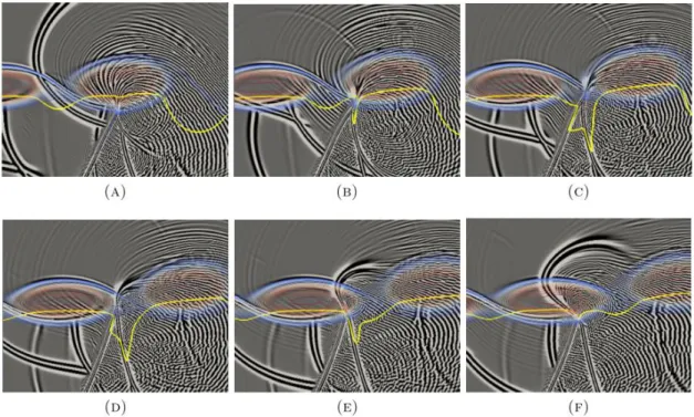
As Screech is due to interaction between coherent structures in the mixing layer and the shock waves. It is important to understand one of the results of this interaction known as shock leakage. Under certain situations, compression waves do not stay confined inside the jet potential core and a part of their energy is released as pressure waves, producing noise. This “escape” is known as shock leakage. Suzuki & Lele (2003), in their numerical and 2D work, have pointed out that the “shock leakage” is an interaction between shock and turbulence processes, where the shocks pass through a vortex-laden mixing layer, as can be seen in fig. 1.9 (Daviller et al., 2013). The saddle point between two eddies allows for pressure waves to escape while the vortices are passing. In the frames “D-F” of the fig. 1.9, it is possible to observe that the pressure waves propagate in the upstream direction of the flow and possibly feed the Screech feedback mechanism. Thus, it appears that shock leakage occurs when the local vorticity weakens (Edgington-Mitchell et al., 2014b).

Figure 1. 9: instantaneous snapshots of shock leakage dynamic. Daviller et al. (2013). Suzuki & Lele (2003) also noted that as the jet temperature increases it is easier for the shocks to penetrate the mixing layer, improving the shock leakage dynamics. Moreover, when the large coherent structure is broken down into the smaller structures the saddle points does not seem to be formed and the shock waves are scattered by the turbulence (Lee et al., 1993). Thus broadband shock noise is generated. Finally, Savarese (2014) pointed out that shock leakage phenomena has never been observed experimentally, only numerical studies were able to provide this behaviour and, up to 2017, shock leakage has still not been experimentally visualised. If found to the contrary, the author is not aware of this.

1.1.3.2 Shock Oscillations

Shock wave oscillations at screech frequencies were cited by Lassiter & Hubbard (1954) through a shadowgraph technique. With the same idea the shock-noise theory of Harper-Bourne & Fisher (1973) was based on the experimental observation that shock behaviours are correlated with the broadband shock noise component (BBSAN). Sherman et al. (1976), using a Schlieren analysis for shock distortion, noticed a relation between shock oscillations and Screech frequencies.

Later, Panda (1998) showed those shock oscillations in his work by laser light scattering acquired by Photo-Multiplier Tube, for two jet conditions (Mj =1.19 and 1.42), involving

axisymmetric and helical Screech modes, respectively. He noticed that the motion of the shocks is more important in the jet core than close to the shear layer. However, this behaviour does not agree to what is expected, as the shock/vortices interaction at shear layer yields more flow unsteadiness. This may be explained by “damping” caused by the shock leakage phenomenon, for example. In his work, Panda showed that the first shock-cell does not have a large oscillation, contrary to the other ones. Another important result is that the mode fashion (fig. 1.10) and frequency of oscillations are the same of the Screech tone. The fig. 1.10 shows nine radial shock positions, on the third cell, for Mj=1.42 and at the different phases of Screech cycle

(τ/Ts). Considering the jet under helical mode, it is possible to see that there is a phase

difference of about 180° in the shock oscillation (the lower half disappears at τ/Ts =0.17 and

appears at 0.83). This behaviour is important because it shows that the shock/turbulence interaction has an important role in the Screech mechanism.

Figure 1. 10: phase-average PMT data obtained at nine radial positions, on third shock in Mj=1.42 and at the different phases of Screech cycle (τ/Ts). Panda (1998).

Panda also observed that the interaction between shock and large organized vortices causes shock splitting into two weaker ones, corroborated by Westley & Wooley (1968, 1970) who observed, by Schlieren film visualisations, that the interaction leads to a generation of a new shock. A possible explanation of the shock splitting is that when a vortical structure spills over the shock, the associated pressure fluctuations due to the passage of these structures are generated as well as a distortion of the super/subsonic interface. Hence, this oscillation may yield important information about large coherent structure turbulence, responsible for the Screech mechanism.

Finally, shock oscillations were also studied by André et al. (2011, 2012), in round convergent jets. In the former work, the authors apply an algorithm to high-speed Schlieren images for shock tips detection at the first and second cells and observed that the shock oscillation occurs at almost the same frequency than the Screech, as can be seen in fig. 1.11. In this image one can notice that the PSD (Power Spectral Density) of the near-field pressure and the shock location signal shows almost the same peak Screech frequency. Hence, we remark that the shock motion in the jet is linked to the Screech mechanism.

Figure 1. 11: PSD (Power Spectral Density) of near-field microphone signal (gray) and PSDx105 of the signal of containing the axial location at the first shock tip at NPR 2.27 (black).

André et al. (2011).

1.2

Screech

The present section provides a review about Screech noise where the main aspects concerning the phenomenon are presented.

1.2.1 Underexpanded Jet Noise in Convergent Nozzle

According to Tam & Tanna (1982), the difference between convergent-divergent and convergent nozzles, concerning the operating conditions, is that the latter always underexpands while the former may be operated at under, over or design conditions. In their work, the authors showed that the minimum noise generation occurs when the nozzle operates at fully expanded condition (fig. 1.12), as in this case, the shock associated noise component is not present.

Figure 1. 12: noise intensity for nozzles undergoing different operating conditions. Tam & Tanna (1982).

The supersonic jet noise in imperfectly expanded flows, as already cited, is formed by turbulent mixing noise, broadband shock-associated noise (BBSAN) and Screech tones, where the two latter are linked to shock-cell structures and known as shock associated noise. André (2012) showed a typical far-field noise spectrum for the convergent nozzles with these three components identified (see fig. 1.13).

Figure 1. 13: typical jet noise spectrum of underexpanded nozzle in far field at Mj=1.35. The black line represents mixing noise, red line the broadband noise, blue line the screech noise and

green line is the combination between mixing and broadband noise. André (2012).

1.2.2 Screech Modes and Staging

As Mj increases the Screech phenomena presents a curious behaviour for round and

elliptical jets: frequencies jumps and structures shifts. These “stages”, visualized as “jumps” in the Screech frequency curve, are called Screech modes and are classified according to jet mode instability. Powell (1953a) identified, for round jets, 4 screech modes that he named A, B, C and D. We report in fig. 1.14 the Screech frequency as a function of Mj from Panda et al. (1997), where the different modes are represented.

Figure 1. 14: screech modes for a circular convergent nozzle. Panda et al. (1997). Powell (1953a) also showed that there is a hysteresis phenomenon between modes C and D, and that the transition from modes A to B is very large with respect to the shift in the frequency. Merle (1956) found that the mode A is constituted of two sub parts, A1 and A2. Panda et al. (1997) found the existence of another mode that they called E. Clem et al. (2012) highlighted new screech modes B’ and F, as can be seen in fig. 1.15. For the rectangular and

elliptical nozzle geometry, Panda et al. (1997) found that for the former the staging behaviour depends on the aspect ratio and the latter presents staging modes called E1, E2 and E3.

Figure 1. 15: fundamental Screech frequency versus Mj for 37.6 mm circular convergent nozzle. Clem et al. (2012)

Powell et al. (1992) employed a Schlieren system for visualisation and microphones to determine the mode organization: A1 and A2 are axisymmetric (or varicose mode), B is flapping (or sinuous), C is helical and D is flapping (or sinuous) too, which confirms previous Powell’s observation. Similar results also were observed by Davies & Oldfield (1962). Nowadays, the mode D is considered to be a mode B extension (Edgington-Mitchell et al., 2015). It means that extrapolating mode B, in the Strouhal x Mj curve, the frequencies for B and D modes match

together. Moreover, mode B is the result of the superposition of two helical modes with opposite signs (Zaman, 1999, Edgington-Mitchell et al., 2015 and Clem et al., 2016).

Powell et al. (1992) also observed the existence of primary (dominant) and secondary Screech frequencies, as shown in fig. 1.16. It is possible to notice that the jet can simultaneously present two frequencies (dominant and secondary). Moreover, Powell et al. showed that there is a hysteresis phenomenon during the transition between modes C and D, as already cited. In this work the authors showed the mode u which they suspected to be the continuation of the mode

A2. However, due to weak tone and a lack of convincing evidence of continuity, this mode was marked as unidentifiable.

Figure 1. 16: screech frequency versus NPR. Frequencies of dominant modes (circles) and secondary modes (crosses). Powell et al. (1992).

Shen & Tam (2002) explained, using different mechanisms of feedback, that it is possible for two modes to coexist, refuting the earlier idea that Screech staging results in a continuous shifting from one mode to another. It is necessary to emphasize that the Screech staging phenomenon is still not completely clear: the physical mechanisms that rule this behaviour still need further study.

1.2.3 Mechanism

As already mentioned, the mechanism of Screech generation is cyclic. It consists of a looping behaviour with 4 phases: 1) perturbations (instabilities waves) increasing within the mixing layer and propagating downstream. They constitute the energy source of the Screech feedback loop (Tam, 1995); 2) shock/turbulence interaction; 3) backward propagation of acoustic waves, and; 4) instabilities re-excitation close to jet exit, restarting the loop (see fig. 1.17), where at this location the thin layer makes instabilities more susceptible to excitation (Kandula, 2008). The first description of the Screech feedback loop was provided by Powell (1953a). Raman (1997) presented Schlieren images of these phases (fig. 1.18) in his work about Screech suppression.

Figure 1. 17: diagram of screech loop (solid lines) and associated phenomena (dashed lines). Raman (1999).

Figure 1. 18: Schlieren image of rectangular nozzle operating in screech loop. Mj = 1.5. Raman (1997).

Shen & Tam (2002) proposed that the feedback phenomenon may be closed by two kinds of disturbances propagating upstream, suggesting that 2 different closure mechanisms may exist. The first mechanism is depicted in fig. 1.19 and it was proposed by Tam et al. (1986). The weakest link feedback loop model, consists of interactions between the shock cell and amplified disturbances that generate acoustic perturbations propagating upstream, outside

of the jet shear layer, reflecting on the nozzle lip and exciting new instabilities. For this model

of feedback, Shen & Tam found a good agreement for the modes A1 (axisymmetric) and B (flapping), meanwhile the results for the modes A2 (axisymmetric) and C (helical) are poorly predicted. It is the classical or standard model of the Screech closure mechanism, also proposed by Powell (1953a).

Figure 1. 19: sketch of the first Screech closure mechanism (classical model).

The second mechanism (fig. 1.20) is based on the presence of another kind of upstream instability waves, with spatial support inside and outside of the jet, identified by Tam & Hu (1989). Employing this model, Shen & Tam could predict the frequency of modes A2 (axisymmetric) and C (helical). Recently, Edgington-Mitchell et al. (2018) showed the signature of this kind of instabilities for both axisymmetric modes A1 and A2, indicating that these upstream-travelling disturbances may close the Screech feedback mechanism of all axisymmetric Screech tones.

Figure 1. 20: sketch of the second Screech closure mechanism (jet modes).

According to Shen & Tam (2002), the presence of these two feedback models explains the coexistence of two Screech tones simultaneously. Later, Chatterjee et al. (2009) found that two feedback mechanisms are associated to two different length scales. The first one (classical) is linked to shock cell spacing and the second one (waveguide model) is bonded to the standing wavelength. Moreover, Edgington-Mitchell et al. (2015) pointed out that the jump in Screech frequency, for elliptical nozzles, may be associated to the transition between different acoustic feedback mechanisms.

To resume, the closure mechanism is still a debated question. No work in the literature has identified the signature of the second Screech closure in the modes B and D. Furthermore, Gojon et al. (2018) observed these waves in a numerical simulation but, no experimental observation is available for the mode C. If found to the contrary, the author is not aware of this.