HAL Id: hal-01957280
https://hal.archives-ouvertes.fr/hal-01957280
Submitted on 17 Dec 2018
HAL is a multi-disciplinary open access
archive for the deposit and dissemination of sci-entific research documents, whether they are pub-lished or not. The documents may come from teaching and research institutions in France or abroad, or from public or private research centers.
L’archive ouverte pluridisciplinaire HAL, est destinée au dépôt et à la diffusion de documents scientifiques de niveau recherche, publiés ou non, émanant des établissements d’enseignement et de recherche français ou étrangers, des laboratoires publics ou privés.
Modelling, Evaluation and Biomechanical Consequences
of Growth Stress Profiles Inside Tree Stems
Tancrède Alméras, Delphine Jullien, Joseph Gril
To cite this version:
Tancrède Alméras, Delphine Jullien, Joseph Gril. Modelling, Evaluation and Biomechanical Conse-quences of Growth Stress Profiles Inside Tree Stems. Anja Geitmann, Joseph Gril. Plant Biomechan-ics. From Structure to Function at Multiple Scales, Springer International Publishing, pp.21-48, 2018, 978-3-319-79098-5. �10.1007/978-3-319-79099-2_2�. �hal-01957280�
Modelling,
Evaluation and Biomechanical
Consequences
of Growth Stress Profiles Inside
Tree
Stems
Tancrède Alméras, Delphine Jullien and Joseph Gril
Abstract The diameter growth of trees occurs by the progressive deposition of
new wood layers at the stem periphery. These wood layers are submitted to at least two kinds of mechanical loads: maturation stress induced in wood during its forma-tion, and the effect of the increasing self-weight. Interaction between growth and these loads causes mechanical stress with a particular distribution within the stem, called growth stresses. Growth stresses have technical consequences, such as cracks and deformations of lumber occurring during sawing, and biological consequences through their effect on stem strength. The first model for computing the field of stress inside a growing stem was set long ago by Kübler. Here, we extend these analytical formulations to cases with heterogeneous wood properties, eccentricity and bending stresses. Simulated profiles show reasonable agreement with measured profiles of released strains in logs. The particular shape of these profiles has consequences on stem bending strength. During bending in response to transient loads such as wind, most of the load is supported by outer parts of a stem cross section. The tensile maturation stress at this level increases the bending strength of the stem by delaying compression failure. Compressive stress in reaction to this tension does not reduce the bending strength because it is located near the centre of the stem and thus not loaded during bending, except if growth is strongly eccentric. Permanent bending stresses are concentrated at the mid-radius of the section, so that they do not cumulate with above-mentioned sources of stress. This smart distribution of stresses makes it possible that the stem is stronger than the wood it is made of, and that a growing stem can bend considerably more than its non-growing beam equivalent without breaking.
T. Alméras (
B
)· D. JullienLMGC, CNRS, Université of Montpellier, Montpellier, France e-mail: tancrede.almeras@umontpellier.fr
J. Gril
CNRS, Université Clermont Auvergne, SIGMA Clermont, Institut Pascal, Clermont-Ferrand, France
J. Gril
Introduction
Like most plants, tree growth occurs by the progressive accumulation of new elements, either the formation of new stem and root portions (primary growth) or their thickening by deposition of new layers of wood or bark (secondary growth). Tree growth stress refers to the distribution of mechanical stress present in the wood of tree stems and branches, as a result of their growth (hereafter we will always refer to stems, but all considerations exposed here apply to both stems and branches). It is caused by the combined effect of permanent weight accumulation and dimensional changes induced by the maturation process during wood formation in the cambial zone (Archer 1986). The mechanisms involved during the maturation process, at the cellular and molecular levels, will be ignored in this chapter; a discussion on that subject is available, for instance in Alméras and Clair (2016). The viewpoint will be essentially that of stem portions, considered as slender structures subjected to normal or bending loads at all stages of development. At the macroscopic level that will be considered here, wood can be considered as a continuous solid medium, characterized by a high degree of anisotropy with an extreme dominance of the fibre direction in terms of rigidity and strength (the fibre directions will be assumed aligned with the stem axis). As a result, the stress distribution within a cross section of the stem can be analysed in this direction only.
The existence of tree growth stress has been initially recognized through its tech-nological consequences, such as checks at log ends after crosscutting, or lumber distortion after sawing (Jacobs 1945). The strain release resulting from any cutting operation, combined with information on wood constitutive equations, is also the usual way to estimate the growth stress. Later biomechanical functions of matura-tion stress have been identified, and can be classified as ‘skeletal’ and ‘motor’ by analogy with animals (Moulia et al. 2006). The motor function refers to the control of tree posture, (i.e. the shape and orientation of its axes), enabled by an asymmetric dis-tribution of maturation stress around the stem circumference. The skeletal function refers to its effect on stem strength (Bonser and Ennos 1998), as will be illustrated in the present paper.
Kübler (1959a,b) was the first to propose a mechanical model of growth stress distribution, which was very useful to analyse either technological or biomechanical aspects. Although the general mechanical framework of stress generation in a grow-ing stem has been well/extensively described in later works (Archer 1986; Fournier et al. 1991a,b), including general numerical formulations (Fourcaud and Lac 2003; Ormarsson et al. 2010). There is a need to return to analytical formulations extending from the initial one by Kübler as they allow straightforward links with parameters describing the growth conditions. The aim of this work is to summarize a number of available models corresponding to typical growth histories, such as radial variations of maturation stress or elastic modulus, eccentric growth with tangential variations of maturation stress (as due to reaction wood formation), bending stresses induced in an inclined stem by passive bending under the self-weight or active uprighting.
Stress profiles computed for these different situations will be shown and compared to measured profiles, and their implication on stem strength will be discussed.
Model:
Computing the Stress Profile Inside Growing Stems
In this section, we state hypotheses on which the calculations are based, derive related equations, and show case studies of application to different situations. The first section (“General Principles of the Mechanics of Growing Stems”) is dedicated to general assumptions underlying the mechanics of a growing structure. Hypotheses formulated in this section will be kept in all case stud-ies. Next sections present case studies of a vertical axisymmetric stem loaded either by its self-weight (section “Case of a Straight and Vertical Axisymmetric Stem Loaded by Its Self-weight”) or by maturation (section “Case of a Straight and Vertical Axisymmetric Stem Loaded by Wood Maturation”), with different patterns of radial distribution of wood properties. Next, the condition of axisymmetry will be released by considering the effect of axial maturation load for an eccentrically growing stem with circumferential variations in wood properties (section “Case of an Actively Reacting Stem with Stationary Orientation”). Finally, the case of a stem bending under the self-weight will be considered (section “Case of a Stem Passively Bending Under Its Self-weight”), as well as the case where the stem both bends and reacts (section “Case of a Stem Bending While Reacting”).
General
Principles of the Mechanics of Growing Stems
The radial growth of a stem is achieved by the cambium. Cambial cells divide and enlarge, increasing the volume of the stem. The cambium is located at the outermost surface of the wood and its thickness is generally very small compared to the section’s diameter. From a macroscopic perspective, the growth of the stem can be viewed as the deposition of new wood layers on the existing wood. The increase in stem volume is thus not described as occurring through deformations of the existing material, but through the accretion of new material at its surface. As a consequence, large strains of existing material are not necessary to achieve large volume changes. The problem will be set in the framework of small strains and linear elasticity.
Modelling Additive Growth with Pre-stresses (H1) The material is loaded only since it was created.
The mechanical stress σ at position x and time t is equal to the sum of an internal stress developing in response to the formation process (the maturation stress σ0) and
external stress increments that have occurred since its formation
σ (x, t )! σ0(x, t ) + t ! tx ∂σ (x, τ ) ∂τ dτ (1)
where tx is the time when the material point located at x was created. (H2) The material has a linear elastic behaviour.
In an elastic context, this pre-stress can be accounted for by using Hooke’s law with prescribed strain
σ ! E(ε − α0)! Eε + σ0 (2)
where σ is the elastic stress, α0is the prescribed strain, ε is the deformation relative to
the configuration of the material at its creation, i.e. before maturation and subsequent loading occur, (ε− α0) is the elastic strain, σ0 ! −Eα0 is the initial stress and E is
the material stiffness (or elastic modulus for 1D formulations).
After a material point is formed (i.e. a new elementary volume is added at the stem surface), it undergoes a phase of maturation during which its density, stiffness and state of stress change and reach a final value. This phase is relatively fast (between a few of weeks and a couple of month) compared with the characteristic time of growth, implying that the ring of immature wood at the stem surface has a negligible thickness compared to the diameter of the stem and its increase during growth. As a consequence, we assume that
(H3) The induction of pre-stress is instantaneous.
σ0(x, t )! σ0(x, tx)! σ0(x) (3) Equation (1) becomes σ (x, t )! σ0(x) + t ! tx ∂σ (x, τ ) ∂τ dτ (4)
The differential form of Eq. (2) is ∂σ (x, t ) ∂t ! E(x) ∂ε(x, t ) ∂t + ∂σ0(x, t ) ∂t ! E(x) ∂ε(x, t ) ∂t (5)
(H4) Size can replace time to describe growth in a monotonously growing structure.
Because the volume always increases during growth, any volume of the structure is associated to a unique time (when the structure reached this volume). As time by itself is not involved in the constitutive Eq. (2), the volume can be used to monitor the succession of events, i.e. the progressive changes in stress
t ! tx ∂σ (x, τ ) ∂τ dτ ! V ! Vx ∂σ (x, u) ∂u du (6)
Equation (4) then becomes
σ (x, V )! σ0(x) + V ! Vx ∂σ (x, u) ∂u du (7)
where Vxis the volume of structure when the material point located at x was created.
Assumptions for a Growing Stem: Beam Theory
(H5) As the stem is a slender structure, beam theory will be used to derive the model.
We are here concerned only by the distribution of longitudinal stress, so that a 1D formulation will be used, where mechanical parameters mentioned above (ε, σ, α0, σ0,E) are scalar. In the context of beam theory, the field of stress is
com-puted for a cross section far enough from the stem ends. The location of a point within the section is (x, y). The increment in strain field within the section is plane. Here, we assume that the change in curvature involves a rotation around the Y axis. The strain increment δε in response to the addition of a new layer of material between t and t + δt is
δε(x, y, t )! δεO(t )− (x − xO)δC(t ) (8) where δεO is the strain at a reference point of the section (typically the pith or the geometrical centre) located at abscissa xO and δC is the change in curvature.
Case
of a Straight and Vertical Axisymmetric Stem Loaded by
Its
Self-weight
Here we assume that the tree is submitted only to the effect of self-weight, neglecting maturation stress. This situation is virtual since wood maturation always occurs
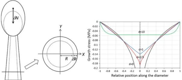
Fig. 1 Case of a vertical and straight stem with circular and homogeneous cross section, loaded by its own weight. In this case, wood maturation stress is neglected. Calculations are made for a stem growing allometrically, exponents d representing the relation between stem radius and length (Eq.18) related to self-weight (Eq. 19). The case d ! 0 represents a stem growing only in diameter, yielding a log profile with asymptotic behaviour at the centre. The infinite value at this level is an artefact of the model, as commented in section “Case of a Straight and Vertical Axisymmetric Stem Loaded by Wood Maturation”. The case d ! 2/3 represents the allometry for elastic stability (Greenhill1881), and the case d ! 1 isometric growth. In these two cases, the profile has a V shape. Large values of the exponent (here d ! 10) represent the case where extension growth is much faster than radial growth. In this case, the profile is uniform in most of the section, tending to the uniform profile expected for a beam without radial growth. The computation has been made for a given stem dimension and weight, but the magnitude of the profile (not its shape) is actually depending on stem size. The mean stress in the section depends on its height (Eq. 25). This mean stress has very low magnitude (for reference, the strength of wood is several tens of MPa)
during tree growth, but it will enable the comparison between these two sources of stress. The tree is assumed straight and vertical and therefore submitted to purely axial loads, with circular and homogeneous cross section (Fig. 1). The first two subsections state hypotheses suitable for this case, but also for some cases presented in sections “Case of a Straight and Vertical Axisymmetric Stem Loaded by Wood Maturation” and “Case of an Actively Reacting Stem with Stationary Orientation”.
Assumptions for a Stationary Stem: Pure Axial Loading
We define as “stationary” a stem whose shape (curvature) does not change during growth. This is the case, for example of a vertical stem that remains vertical. It is also the case of a leaning stem for which lean and shape remain constant, because the effect of weight increment is compensated by the active reaction (asymmetry of maturation stress within the section), or, for example because bending is prevented by a stalk.
Let us assume that the stem is submitted to a normal force increment δN (t), as due, for example to weight or maturation load. As we assume that only axial contraction occurs (δC ! 0), the strain increment is uniform over the section
δε(x, y, t )! δεO(t ) (9)
The strain increment due to the normal force increment is
δεO(t )! δN(t)/" ¯E(t ) A(t )# (10) where A(t) is the section area and ¯E(t) is the homogenized modulus of elasticity
given by
¯E(t) ! !
δS
E(x, y)dxdy$A(t) (11) Considering the incremental form of the constitutive Eq. (2), δσ ! Eδε, together with Eq. (10), the stress increment in response to the load increment is
δσ (x, y, t )! δN (t)
A(t) E(t)
¯E(t) (12)
Formulation for a Circular Homogeneous Cross Section
For a circular cross section, the section geometry can be characterized by its outer radius R and this variable can be used to monitor time. Because the loading is purely axial, the problem is axisymmetric, and the position of a point is characterized by its radial position r. Therefore, coordinates (x, y, t) become (r, R), where R is the radius of the stem at time t. Neglecting maturation stress, Eq. (1) becomes
σ (r, R)! R ! r ∂σ (r, u) ∂u du (13)
As the elastic modulus is homogeneous, we have ¯E ! E, so that Eq. (12) becomes δσ (r, R) ! δN (R)
A(R) (14)
For a circular cross section, we have A(R)! π R2, so that Eq. (14) becomes
δσ (r, R) ! δN (R)
πR2 (15)
∂σ (r, R) ∂R ! 1 πR2 d N (R) d R (16)
Finally, the relation between growth stresses and the evolution of axial loading is
σ (r, R)! 1 π R ! r d N (u) du u−2du (17)
Application to Stem Allometric Growth
Let us assume that the tree grows in radius R and length L following an allometric law given by
L ! cRd (18)
The normal force induced by self-weight N is assumed proportional to the volume of the stem and expressed as
N ! −kπ R2L ! −kπcRd+2 (19)
where k ! N/"πR2L#is a constant linking stem weight to stem dimensions, account-ing for the effect of taper, branch distribution and density.
Deriving with respect to R, we obtain
d N (R)
d R ! −kπc(d + 2)R
d+1 (20)
Substituting into (17), we obtain the field of stress within the section
σ (r, R)! −kc(d + 2) R ! r ud−1du (21) Which integrates as σ (r, R)! −kc(d + 2) d " Rd − rd# for d ̸! 0 (22) σ (r, R)! 2kcln(r/R) for d ! 0 (23)
We define the relative radius ρ
ρ ! r/R (24)
¯σ ! N (R)A(R) ! −kcπ Rd
+2
πR2 ! −kcR d
! −kL (25)
Equations (22) and (23) can be rearranged as σ (r, R)! ¯σd + 2
d
"
1− ρd# for d ̸! 0 (26)
σ (r, R)! −2 ¯σlnρ for d ! 0 (27)
Results are shown and commented on Fig.1.
Case of a Straight and Vertical Axisymmetric Stem Loaded by
Wood Maturation
Here we compute the field of growth stress of a straight and vertical tree with circular cross section submitted to maturation stress, neglecting the self-load (Fig. 2). The problem is axisymmetric and equations derived in section “Assumptions for a Sta-tionary Stem: Pure Axial Loading” still apply. First (Section “Kübler’s Model”) we will derive Kübler’s model assuming uniform properties (maturation stress and elas-tic modulus) within the section. Next, the assumption of uniformity will be released, by considering radial variations in either maturation stress (Section “Case of Poly-nomial Radial Variations of Maturation Stress”) or elastic modulus (Section “Case of Linear Radial Variations of Elastic Modulus”). As only radial variations are con-sidered, the problem is axisymmetric and coordinates (r, R) will be used to refer to radial position r when the stem has radius R.
Kübler’s Model
Because the problem is axisymmetric and maturation stress is uniform Eq. (4) becomes σ (r, R)! σ0+ R ! r ∂σ (r, u) ∂u du (28)
The normal force resulting from maturation stress in the section increment between R and R + δ R is δN (R)! − ! δS σ0du ! −σ0 ! δS du ! −2π RδRσ0 (29)
Fig. 2 Case of a straight and vertical stem with circular and homogeneous cross section, loaded
by wood maturation (Kübler’ model). Here, the stem self-weight is neglected. The figure shows the growth stress profile, for different values of maturation stress: 5 MPa (continuous line), 10 MPa (dashed line) and 15 MPa (dotted line). Profiles have a typical log shape, with the value of maturation stress in the periphery (tension), a null stress located at 0.6 times the radius, and strong compression in the core. Profiles are self-similar (i.e. the pattern does not depend on stem size), and balanced (i.e. the integral over the whole section is null). The magnitude of stress is several orders of magnitude larger than that of self-weight (Fig.1), providing an a posteriori verification of the assumption that self-weight has a negligible effect. The infinite value at the centre of the section is an artefact due to the mathematical formulation of the model, because the profile is integrated since R! 0, whereas the stem has finite size at the very beginning of radial growth, with tissues other than wood having a dominant contribution to stem stiffness
d N (R)
d R ! −2π Rσ0 (30)
Using Eq. (16), we obtain ∂σ (r, R) ∂R ! 1 πR2 d N (R) d R ! −2 σ0 R (31)
Substituting in Eq. (28) and defining ρ ! r/R, we obtain
σ (r, R)! σ0 − R ! r 2σ0 u du ! σ0(1 + 2 ln(ρ)) (32)
Results are shown and commented on Fig.2.
Case of Polynomial Radial Variations of Maturation Stress
Here, we still consider the axisymmetric problem of a vertical and straight tree with circular cross section (Fig. 2), but account for possible radial variations in
maturation stress. This problem may represent the case of a tree with ontogenic or environmental changes inducing variable level of maturation stress during growth.
We assume that the radial change in maturation stress during growth has polyno-mial form σ0(r )! N % 0 anrn (33)
This can describe any pattern of variation.
For a non-uniform pattern of maturation stress in axisymmetric case, Eq. (4) becomes σ (r, R)! σ0(r ) + R ! r ∂σ (r, u) ∂u du (34)
Substituting Eqs. (33), (31) becomes ∂σ (r, R) ∂R ! −2 N % 0 anRn−1 (35)
The growth stress profile is obtained by combining Eqs. (33), (34) and (35)
σ (r, R)! N % 0 anrn − 2 N % 0 an R ! r un−1du (36) Which integrates as σ (r, R)! N % 1 & 1 + 2 n ' anrn − 2 N % 1 an n R n + a 0 ( 1 + 2 ln( r R )) (37) Defining the relative radius ρ ! r/R, this can be rearranged as
σ (r, R)! a0(1 + 2 ln ρ) + N % 1 anRn && 1 + 2 n ' ρn − 2 n ' (38) Results are shown and commented on Fig.3.
Fig. 3 Results for the same situation as Fig.2, but with non-homogeneous patterns of radial vari-ations in maturation stress (a monotonous varivari-ations; c non-monotonous varivari-ations). The matura-tion stress patterns represent possible scenario of response to ontogenic or environmental changes (Jullien et al.2013; Dassot et al.2015). Simulations (b, d) show that the shape of growth stress profiles can differ substantially from Kübler’s model. The shape generally presents asymptotic infi-nite negative value on the middle of the section, which is a mathematical artefact of the model. The case where maturation stress is small in early stages (a, dotted lines) don’t show this asymptotic behaviour and is convex with a U shape. For non-monotonous variations in maturation stress growth stress profiles show a variety of shape, either convexo-concave or even non-monotonous along a radius
Case of Linear Radial Variations of Elastic Modulus
Here, we still consider the axisymmetric problem of a vertical and straight tree with circular cross section (Fig. 2), but account for possible radial variations in elastic modulus. This problem may represent the case of a vertical and straight tree with ontogenic variations of the modulus of elasticity, as typically happens for conifers in juvenile stages.
We assume that the change in elastic modulus during growth has linear form
E(r)! ar + b (39)
The maturation strain is assumed uniform. The maturation stress is then non-uniform and is
For nonuniform elastic modulus, Eq. (11) becomes ¯E(R) ! 2π ! 0 R ! 0 u E(u)dudθ/ 2π ! 0 R ! 0 ududθ ! 2 3a R+ b (41)
Applying the same principle as (H1) to the growth strain profile, and reminding that ε is the strain since initial configuration (i.e. the initial strain is 0 by definition of ε) Eq. (1) is replaced by ε(r, R)! R ! r ∂ε(r, u) ∂u du (42) Equation (10) becomes δε(r, R) ! δN (R) ¯E(R)A(R) ! 2π Rα0E(R)δ R πR2 ¯E(R) ! 2α0 a R+ b 2 3a R2 + bR δR (43) Therefore, ∂ε(r, R) ∂R ! 2α0 a R+ b 2 3a R2 + bR (44) The strain profile is obtained by combining Eqs. (42) and (44)
ε(r, R)! 2α0 R ! r au+ b (2/3)au2+ budu (45) Which integrates as ε(r, R)! −α0 & 2 ln(r/R) + ln & (2/3)ar + b (2/3)a R + b '' (46) Combined with Eqs. (2) and (39), the stress profile can be deduced
σ (r, R)! −α0(ar + b) & 1 + 2 ln(r/R) + ln & (2/3)ar + b (2/3)a R + b '' (47) Results are shown and commented on Fig.4.
Fig. 4 Results for the same situation as Fig.2, but with non-homogeneous patterns of radial vari-ations in modulus of elasticity (a) representing, for example the case of a conifer in juvenile stage. The stress profile (b, solid red line) is close to linear along a radius. However, because the MOE is heterogeneous, the shape of the released strain profile (b, green dashed line) is different and closer to Kübler’s model
Case of an Actively Reacting Stem with Stationary Orientation
Here, we consider a non-axisymmetric problem where tangential variations of mat-uration stress and growth increments occur (Fig.5). Particular cases (only tangential variations in maturation stress or only eccentric growth) are encompassed by this formulation. This problem is no more axisymmetric. The stem is assumed station-ary, i.e. not submitted to changes in curvature during growth, and thus loaded only axially. This corresponds to a tilted stem that remains tilted at constant angle, and, therefore, undergoes no bending. This situation typically happens for a staked stem or for branches where the reaction exactly compensates for the effect of increasing weight.
Let us consider a circular cross section growing by addition of eccentric layers, but remaining circular during growth. We also assume homogeneous elastic properties within the cross section. Here the position of the pith is not at the centre of the section. Let xO be position of the centre of the section relative to pith at a given time. During growth, this position moves relatively to the pith. The pith is taken as a reference because the position of a material point is fixed in this reference. Let δxO be the displacement of the centre during the addition of a growth ring increasing the section’s diameter by δ D. Let δ R be the half of diameter increment. The eccentric growth is characterized by parameter kO such that
kO ! δxO/δR (48) Assuming that the section grows with constant eccentricity since the beginning of growth, the position of the geometric centre can be obtained by integration
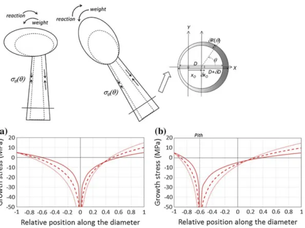
Fig. 5 Case of a “stationary” stem (i.e. a stem keeping constant shape) reacting to eccentric growth
and the production of tangential variations in maturation stress. The stem can be vertical or tilted, provided the load caused by the self-weight is exactly compensated by the load caused by the reaction. Cases with no eccentricity and various levels of maturation stress on the tension wood side are shown on chart (a). Profiles have a log shape, with possible shift between the two sides, due to the asymmetry in maturation stress. Cases with eccentricity are shown on chart (b). Profiles still have a log shape, but with marked asymmetry between the two sides. Note that the maximal compressive stress is located at the pith, not at the geometric centre of the section
The tangential distribution of the radius increment is approximated as
δR(θ) ! δR(1 + kOcos θ) (50)
The tangential distribution of the maturation strain and stress is given as αO(θ )! ¯α + 1 2*αcos θ (51) σO(θ ) ! ¯σ + 1 2*σ cos θ (52)
With ¯σ ! −E ¯α and *σ ! −E*α. Here, the modulus E is assumed uniform.
Let us consider a point of the section located in (x, y) in a reference attached to the pith. Equation (7) becomes
σ (x, y, R)! σ0(x, y) + R ! rx y ∂σ ∂udu (53)
where rx y is the mean radius of the section when the point located in (x, y) was created. Equation (14) becomes δσ (x, y, R)! −δN (R) A(R) (54) Equation (29) becomes δN (R)! δR 2π ! 0 σ0(θ )(1 + kOcos θ)Rdθ (55)
Substituting Eq. (52), we obtain
δN (R)! RδR 2π ! 0 & ¯σ + 12*σcos θ ' (1 + kOcos θ)dθ (56) Which integrates as δN (R)! RδR ( 2π¯σ + π 2kO*σ ) (57) Reminding that A(R)! π R2 and combining with (54), Eq. (31) becomes
∂σ (x, y, R)
∂R !
2¯σ + 12kO*σ
R (58)
Let us compute the stress profile at the level of the axis of symmetry (y ! 0). For x > 0, y ! 0, the maturation stress is
σ0(θ ) ! ¯σ + 1
2*σ (59)
From Eq. (48), it can be deduced that
rx y ! x/(kO + 1) (60)
σ (x, 0, R)! ¯σ + 1 2*σ + R ! x/(kO+1) 2¯σ + 1 2kO*σ u du (61) Which integrates as σ (x, 0, R)! ¯σ + 1 2*σ + & 2¯σ + 1 2kO*σ ' ln & x R kO + 1 ' (62) For x < 0, y ! 0, the maturation stress is
σ0(θ ) ! ¯σ −
1
2*σ (63)
From Eq. (48), it can be deduced that
rx y ! x/(kO − 1) (64)
Substituting Eqs. (58), (63) and (64) into (53)
σ (x, 0, R)! ¯σ − 1 2*σ + R ! x/(kO−1) 2¯σ + 1 2kO*σ u du (65) Which integrates as σ (x, 0, R)! ¯σ − 1 2*σ + & 2¯σ + 1 2kO*σ ' ln & x R kO − 1 ' (66) Results are shown and commented on Fig.5.
Case
of a Stem Passively Bending Under Its Self-weight
Here, we consider a stem that grows at the same time it bends. In this section, maturation stress is neglected on purpose (Fig. 6). The general problem of a stem submitted to both bending and maturation will be studied in next section. As will be shown, the stress profile only depends on the changes in curvature, not on their cause. The model is therefore valid whether this change in curvature occurs in response to sagging under the self-weight, to uprighting due to maturation stress asymmetry or to any external forcing. The first section is dedicated to general assumptions for a stem changing in curvature. Then, two cases will be studied. First, an axisymmetric section will be considered. This corresponds to the situation where a stem does not react during growth, so that it bends under its self-weight. Note that even if the
Fig. 6 Case of a tilted stem bending under its own weight. The section is circular with homogeneous modulus of elasticity, and possibly eccentric growth. Here only bending stresses are computed, and maturation stresses are neglected on purpose. The calculation was made for different allometric laws of the stem, defined by an allometric exponent between radius and length (Eq. 18). Results are shown for different patterns of eccentricity and different allometric exponents d. a Case with no eccentricity. b Case with eccentricity on the upper side of the tilted stem. c Case with eccentricity on the lower side of the tilted stem. Values of d represent different remarkable cases of allometry: only radial stability gro ( wth Alméras (d ! and 0); F a ournier llometry a 2009) ( ssociated d to 1/2); constant allometry stress associated (McMahon to elastic 1976) or stability biomech (Greenhill anical !
1881) (d! 2/3); isometric growth (d ! 1); situation where radial growth is much slower than weight increase (d ! 10). Case d ! 0 shows asymptotic behaviour near the pith, which is an artefact of the model. Maximal bending stress is located near the pith, tensile on the upper side, and compressive on occur the lo from wer t s he ide. T periphery his loc to atio the n of pith ma in xi t m he a is als concentric o observ case. ed f F or or d d! 1/2,2/3 and where d linear 1, v the ariations profile is sigmoid, with maximal magnitude located in the middle part of t!he radius. T!he case d 10
! shows a linear pattern in most of the section, tending to the usual bending stress profile expected for a non-growing beam. The case where eccentricity occurs on the upper part of the section shows similar but distorted results. For the case d ! 10, the profile is almost exactly the same, and the stress is null at the geometric centre. For other cases, compression is concentrated on the lower side, and its maximal magnitude is larger than in the concentric case. Tension occurs in the part of the section located above the pith, and it maximal value is lower than in the concentric case. When eccentric growth occurs on the lower side, the pattern is inverse: tension is concentrated above the pith and its maximal value is larger than in the concentric case, and compression is concentrated under the pith and its maximal value is lower than in the concentric case
section is axisymmetric, the problem is not axisymmetric because bending occurs. Second, we will consider a non-axisymmetric section with eccentric growth. This corresponds to the situation of a stem in active reaction and uprighting movement (although only the effect of changes in curvature will be accounted for, not the stress directly due to maturation).
Assumption for a Stem Submitted to Changes in Curvature
In both situations of passive bending and active uprighting, the change in curvature associated to an increment in section radius is depending on section’s radius. For the active uprighting, it has been shown (Fournier et al.2006; Alméras and Fournier
2009) that the change in curvature scale at power−2 with the radius. For the passive bending case, we will show that changes in curvature and radius are also related by a power law when assuming a power law for allometric growth (Section “Case of an Eccentric Section”). We assume that the stem undergoes a bending movement during growth, the change in curvature δC that occurs during growth from R to
R+ δ R following a power law δC δR !C
′(R) ! aRb with b
̸! −1 (67)
The problem is no more axisymmetric because of the distribution of bending stresses. Let (x, y) be the position of a point relative to the centre of the section. As the stem is assumed submitted to pure bending around its neutral line, Eq. (8) becomes
δε(x, y, R)! (x − xO)δC(R) (68)
where xO is the position of the neutral line of the section.
Case of an Axisymmetric Section
Here we assume that the section is circular and homogeneous, and compute the stress profile along the diameter parallel to X. From Eqs. (66) and (67), and reminding that the geometric centre and the position of neutral line are equal for an homogeneous section we deduce that
∂ε(x, y, R)
∂R ! xC
′(R) (69)
Combining with Eq. (5) we have ∂σ (x, y, R)
∂R ! ExC
′(R) (70)
Neglecting initial stress in the section, Eq. (7) becomes
σ (x, y, R)! R ! rx y ∂σ (x, y, u) ∂u du (71)
where rx y is the radius of the section when point located at (x, y) was created. Combining Eqs. (66), (69) and (70), we obtain
σ (x, y, R)! x E R ! rx y C′(u)du ! x E R ! rx y aubdu ! ax E b+ 1 " Rb+1 − rb+1 x y # (72)
In particular, for the diameter parallel to X (y ! 0) we have rx y ! x if x > 0 and
rx y ! −x if x < 0.
Defining ρ ! x/R, this can be rearranged as σ (ρ, R)! a E R
b+2
b+ 1 ρ "
1− |ρ|b+1# (73)
Case of an Eccentric Section
Let us consider an eccentric section characterized by parameter kO (Fig.5). Com-bining Eqs. (67), (68) and (49), Eq. (54) becomes
∂ε(x, y, R)
∂R ! (x − kOR)C
′(R) (74)
Equation (54) then becomes ∂σ (x, y, R)
∂R ! E(x − kOR)C
′(R) (75)
Combining Eqs. (71) and (75), the final stress is obtained by integration
σ (x, y, R)! E R ! r C′(u)du− EkO R ! r RC′(u)du (76) Injecting Eq. (67) σ (x, y, R)! aE ⎛ ⎝ x R ! r ubdu− k O R ! r ub+1du ⎞ ⎠ (77) Which integrates as σ (x, y, R)! aE . x"Rb+1− rb+1# b+ 1 − kO"Rb+2− rb+2# b+ 2 / (78)
In particular, for the diameter parallel to X (y ! 0) we have r ! x/(1 + kO) for
x > 0 and r ! x/(1 − kO) for x < 0. Let ρ be the reduced position defined as ρ ! (x/R)/(1 + kO) if x > 0
ρ ! (x/R)/(1 − kO) if x < 0 (79)
Equation (78) can be rearranged as σ (ρ, R)! aE Rb+2 . ρ(1 + kO)"1− ρb+1# b+ 1 − kO"1− ρb+2# b+ 2 / if ρ > 0 σ (ρ, R)! aE Rb+2 . ρ(1− kO)"1− ρb+1# b+ 1 − kO"1− ρb+2# b+ 2 / if ρ < 0 (80)
Application of the Bending Model to Allometric Growth
Let us assume that the tree grows following the same allometric law (L ! cRd) as in section “Application to Stem Allometric Growth” and compute the change in curvature due to the increase in self-weight. The normal force induced by self-weight
N is given by Eq. (19).
Assuming that the centre of mass is located at mid-length of the stem load, the bending moment applied at the base of the stem can be computed
M ! P L/2 ! kc2R2d+2/2 (81)
The bending moment increment in response to a growth increment d R is
d M d R !kc
2
(2d + 2)R2d+1/2 (82)
The change in curvature is then
dC d R !
d M
E I d R !a R
b (83)
Reminding that for a circular cross section I ! π R4/4, we have
b ! 2d − 3 (84)
a ! 2kc
2(2d + 2)
πE (85)
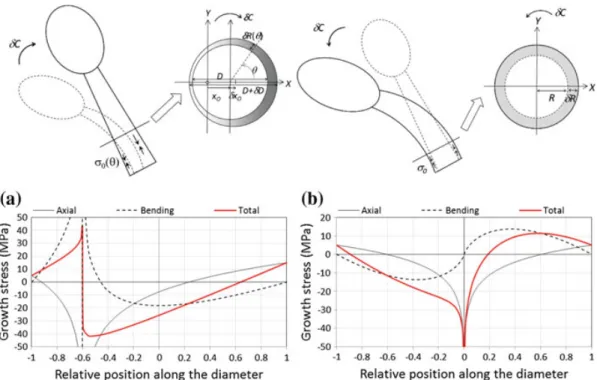
Fig. 7 General case of a stem bending while producing maturation stress. Two cases are illustrated:
case of active up-righting due to asymmetric maturation (a), and case of passive bending under the self-weight due to isometric growth with production of axisymmetric maturation stress (b). Figures show separately stresses due to axial load resulting from maturation (continuous thin black line), stresses due to bending (dotted line) and total stress (thick red line). Stress profiles are asymmetric, with a “ν”-shape (Greek letter nu). In the case of active up-righting, the maximal magnitude of total stress is reduced compared to its individual components (axial and bending stresses)
Case
of a Stem Bending While Reacting
In the general case, a stem always produces maturation stress and is sometimes also submitted to bending stresses. Whether the bending stresses are due to self-weight, active reaction or any combination of these the causes does not change the stress profile, only the variation of curvature during the course of growth matters. For the given section’s parameters, the growth stress profile is simply obtained by adding axial and bending stress profiles. Results are shown and commented in Fig. 7.
Experiments:
Growth Stress Measurements and Model
Validation
Experiments
The study was conducted on four tilted poplar trees located near Montpellier (France). Tree diameter at breast height ranged between 6 and 14 cm. Trees were felled and cut
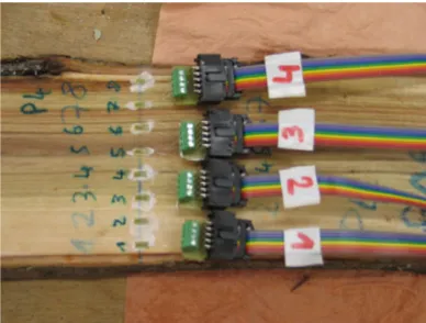
Fig. 8 Measurements of
residual strains of a freshly sawn poplar board. 8 strain gauges are pasted along the grain across the diameter. Growth stresses are later released by operating transverse cuts below and above the gauges, and recording released strains
into logs 10–20 longer than the diameter, before being transported to the laboratory. Logs were stored in a plastic sheet in a refrigerated room, and a diametral board was sawn within a few weeks after felling to avoid drying. The board was oriented along the axis of symmetry of the tilted tree. Across the diameter located at mid-length of the board, 7–11 5 mm-long strain gauges were pasted in the grain direction and connected to a data logger (Fig. 8). Residual strains of growth stresses were released and measured by operating transversal cuts close to each side of the gauges.
Results
and Assessment of the Model
Measured released strain profiles are shown in Fig. 9. The opposite of the strain is plotted, so that a contraction (negative strain corresponding to tensile growth stress) is represented by positive values. Stems had variable degrees of eccentricity (the Y axis corresponds to the pith). In all cases, tension is observed at the periphery and compression near the core, consistently with simulation. For two specimens (P1 and P4), a marked asymmetry of maturation strain (peripheral values of strain) is observed. In contrast with simulated growth stress profiles, we observe finite negative values of strains near the core, less negative and sharp than expected from simulations. This may be due to some nonlinear behaviour near the core, where large compression may be released by viscoelastic and/or plastic behaviour. Consistently with simulations, the maximal compression is mostly located near the pith (except for P4) rather than near the geometric centre of the section.
The variety of profiles observed are likely due to variable patterns of heterogeneity (of maturation stress or elastic modulus) and growth history, as attested by the variety of profiles obtained from simulations. Local increase in stress away from the pith as observed in P1 and P5 are likely due to past temporary reaction or bending movement of the stem.
Fig. 9 Profiles of residual strains (10−6 m/m) measured across the diameter (cm) of four poplar trees. Different shapes are observed, more or less in accordance with simulated profiles, with tensile stress at the periphery and compressive stress near the core. The absence of strongly negative value near the core is likely due to plastic deformations occurring in this area, not taken into account by the models
Discussion
Limits
of the Model and Possible Extensions
In this section, we will review possible extensions of the preceding formulations. In section “Extension of the Formulations”, the case of different geometry or load-ing history, or the refinement of the mechanical analysis will be considered while keeping the general principles stated in part 2.1. In section “Reconsidering the Basic Equations”, their partial release will be considered.
Extension of the Formulations
Using a numerical formulation, the model can be easily extended to any section shape or distribution of mechanical properties or maturation stress within the section. It is, however, still possible to obtain analytical expressions in some cases that were not detailed here
• The constant allometry assumed in section “Application to Stem Allometric Growth” or “Application of the Bending Model to Allometric Growth” can be gen-eralized to more complex situations. Based on the incremental formulation giving the stress increment δσ at a given position in the cross section for an increase of stem size δR, the partial derivative ∂σ/∂R can be obtained and the integration of Eq. (1) can be made. Possible extensions that could also lead to analytical equa-tions, include a change—either progressive or sudden—of the allometry exponent, corresponding to a change of growth condition or of the limiting factor causing the allometry.
• The equations obtained for a circular cross section can be extended to the ellipsoid case by an appropriate change of variable in the computation of surface integrals. Here also a change of the growth conditions, resulting in a progressive or sudden change of circularity, can be introduced without much difficulty.
• The variables appearing in section “Modelling Additive Growth with Pre-stresses” and Eqs. (1–7)—stress σ, strain ε, stiffness E …—have been so far considered as scalars for a 1D formulation. The equations apply equally to 3D formulations, with all the variables becoming tensors. The beam theory for a slender structure, stated in section “Assumptions for a Growing Stem: Beam Theory” and Eq. (8), remains applicable using the formulation of generalized plane deformation as shown for example by Archer (1986) or Fournier et al. (1991a, b) for the case of a circular cross section with concentric growth rings (no eccentricity). These authors assumed orthotropic elasticity and also included in their formulation the torsion resulting from inclined grain. A model of transverse isotropy that neglects the differences between the transverse directions can be also used to simplify the formulations.
Reconsidering the Basic Equations
Except for (H1) (material loaded since created), all basic assumptions made in part 2.1 can be questioned. Linear elasticity (H2) obviously needs to be questioned con-sidering the excessive stress levels predicted by the models near the biological centre of the stem. Elastoplastic models reducing the stress increase above a certain limit (the yield stress) can be introduced (Archer 1986), as well as the apparition of dam-age characterized by a decrease of stiffness. The generation to hollow stems can be addressed through such an approach, by considering that the core of the stem is totally damaged. Such time-independent formulations remain compatible with (H4).
When the viscoelastic behaviour is introduced, (H4) is not valid anymore: the time cannot be replaced by stem size, as there is an explicit dependence on time in the constitutive equations of the material. (H3) no longer applies when the effect of progressive maturation is studied as in Coutand et al. (2007). Viscoelasticity can be used to account for the progressive stiffening of the material during the process of maturation (Gril and Fournier 1993).
Beam theory (H5) can be used to model the movement of the whole stem under the action of internal or external forces. In that case, slow variations of properties
along the stem axis, such as conicity, can be taken into account using the current description applicable to each stem portion. In case slenderness (length to diameter ratio) is not large enough, the effect of shear must be taken into account using the theory developed by Timoshenko (1940). It results in an additional contribution to the stem movement, in proportion to the wood anisotropy characterized by the ratio of longitudinal Young’s modulus (EL) to longitudinal shear modulus (GLTor GLR).
In the long term, due to the higher relaxation in shear compared to that along the fibre, the effective level of anisotropy is likely to increase and the contribution of shear likely to become significant.
Consequences
of Growth Stress Patterns for Stem Strength
Patterns of growth stress always exhibit very nonlinear variations across the diameter. This pattern is in sharp contrast with the linear profile expected for a beam submitted to axial and bending loads. These non-classical patterns are a direct consequence of the interaction between growth and loading: although the stress increment associated to a radius increment has linear variations within the section, the integration of this stress overgrowth is nonlinear. The profile is nonlinear because new wood layers are progressively added to structure, so that each layer has its own loading history: old layers have undergone more load increments than younger peripheral layers.
The state of pre-stressing has direct consequences on stem strength. If a transient bending load is applied to the stem, a linear stress profile is added to the growth stress profile. This additional stress field is maximal at the periphery, compressive on one side and tensile on the opposite side. Peripheral pre-tension reduces compression on the compressive side of the stem, and increases tension on the tensile side. As fresh wood is weaker in compression than in tension, the pre-stress is beneficial for the stem strength. The stem as a structure has larger strength than the wood it is made of. Since peripheral tension is typically 5–10 MPa (compared to a compressive strength typically ranging between 20 and 50 MPa), this strength increase amounts several tens of percent.
The peripheral tensile pre-stress is balanced by a strong compression near the core of the stem. Usually, this does not significantly reduce stem strength, since central parts of the stem bear only negligible bending loads. However, in the case where eccentricity is strong, large compression near the pith is located away from the neu-tral line of the stem. The pith, pre-stressed in compression, may then be additionally loaded in compression during transient bending. A non-classical behaviour may hap-pen in this case, where the mechanical failure starts inside the stem (at the level of the pith) rather than at its periphery. Because stress profiles are often asymmetric, another non-classical behaviour may happen: the strength of the beam is not symmet-ric with respect to the bending direction. Figure 7 illustrates a case where strength is lower for downward movement (where compression away from the pith may add with transient compression) than for an upward movement. Permanent bending stress profiles (Fig. 6) have a particular sigmoid shape. An important point is that although
it has undergone large changes in curvature, the stress is null at the periphery. As a consequence, a growing stem can withstand considerably larger changes in curvature without breaking than its non-growing equivalent. To illustrate this let us compare the case of a stem of diameter R, submitted to a curvature increment C either dur-ing the course of growth or at final state. If the change occurs at final state, then the maximal stress in the section is located at the periphery and can be computed using usual formulae, namely σmax ! E RC, where E is the elastic modulus. For the growing stem, we assume that the rate of change in curvature growth is equal to the rate of change of diameter (b! 0 in Eq.67). Then, the location of the maxi-mal stress can be obtained by deriving Eq. 73, and its magnitude can be expressed as σmax ! 14E RC. Therefore, the maximal curvature that can be achieved by the growing stem is fourfold larger than the non-growing stem.
The state of stress of a stem can be viewed as the sum of three kinds of stress: pre-stress due to maturation at the periphery and associated growth stress in the core; stress due to permanent bending in response to self-weight and/or asymmetric maturation; stress due to transient bending when the stem is submitted to instan-taneous external action. It is noteworthy that these stresses are smartly distributed in the section: maturation stresses are tensile at the periphery, growth stresses are concentrated near the core of the stem, bending stresses are concentrated in the mid-parts of the radius, and transient stresses are located in the peripheral part. Thanks to this smart distribution, a stem that has already undergone large permanent bending movements can also withstand transient bending without loss of strength.
References
Alméras T, Clair B (2016) Critical review on the mechanisms of maturation stress generation in trees. J R Soc Interface 13:20160550
Alméras T, Fournier M (2009) Biomechanical design and long-term stability of trees: morphological and wood traits involved in the balance between weight increase and the gravitropic reaction. J Theor Biol 256(3):370–381
Archer RR (1986) Growth stresses and strains in trees. Springer, New York
Bonser RHC, Ennos AR (1998) Measurement of prestrain in trees: implications for the determination of safety factors. Funct Ecol 12(6):971–974
Coutand C, Fournier M, Moulia B (2007) The gravitropic response of poplar trunks: key roles of prestressed wood regulation and the relative kinetics of cambial growth versus wood maturation. Plant Physiol 144(2):1166–1180
Dassot M, Constant T, Ningre F, Fournier M (2015) Impact of stand density on tree morphology and growth stresses in young beech (Fagus sylvatica L.) stands. Trees 29(2):583–591
Fourcaud T, Lac P (2003) Numerical modelling of shape regulation and growth stresses in trees: I. An incremental static finite element formulation. Trees 17(1):23–30
Fourcaud T, Blaise F, Lac P, Castéra P, De Reffye P (2003) Numerical modelling of shape regulation and growth stresses in trees. Trees 17(1):31–39
Fournier M, Stokes A, Coutand C, Fourcaud T, Moulia B (2006). Tree biomechanics and growth strategies in the context of forest functional ecology. In: Ecology and biomechanics—a mechan-ical approach to the ecology of animals and plants, pp 1–33
Fournier M, Chanson B, Thibaut B, Guitard D (1991a) Mécanique de l’arbre sur pied: modélisation d’une structure en croissance soumise à des chargements permanents et évolutifs. 2. Analyse tridimensionnelle des contraintes de maturation, cas du feuillu standard. Annales des Sciences forestières 48(5):527–546
Fournier M, Chanson B, Guitard D, Thibaut B (1991b) Mécanique de l’arbre sur pied: modélisation d’une structure en croissance soumise à des chargements permanents et évolutifs. 1. Analyse des contraintes de support. Annales des sciences forestières 48(5):513–525
Gril J, Fournier M (1993) Contraintes d’élaboration du bois dans l’arbre: un modèle multicouche viscoélastique, 11ème Congrès Français de Mécanique, vol 4. Association Universitaire de Mécanique, Lille-Villeneuve d’Ascq, pp 165–168
Greenhill A-G (1881) Determination of the greatest height consistent with stability that a vertical pole or mast can be made, and of the greatest height to which a tree of given proportions can grow. Proc Camb Philos Soc IV(Part II)
Jacobs RR (1945) The growth stresses of woody stem. Commonw For Bur Aust Bull 28:1–64 Jullien D, Widmann R, Loup C, Thibaut B (2013) Relationship between tree morphology and growth
stress in mature European beech stands. Ann For Sci 70(2):133–142
Kübler H (1959a) Studien über Wachstumsspannungen des Holzes I. Die Ursache der Wachstumss-pannungen und die SWachstumss-pannungen quer zur Faserrichtung. (Studies of growth stresses in trees Part 1. The origin of growth stresses and the stresses in the transverse direction). Holz Roh-Werk 17:1–9
Kübler H (1959b) Studien über Wachstumsspannungen des Holzes II. Die Spannungen in Faserrich-tung. (Studies of growth stresses in trees Part 2. Longitudinal stresses). Holz Roh-Werk 17:44–54 McMahon TA, Kronauer RE (1976) Tree structures: deducing the principle of mechanical design.
J Theor Biol 59(2):443–466
Moulia B, Coutand B, Lenne C (2006) Posture control and skeletal mechanical acclimation in terres-trial plants: implications for mechanical modeling of plant architecture. Am J Bot 93:1477–1489 Ormarsson S, Dahlblom O, Johansson M (2010) Numerical study of how creep and progressive
stiffening affect the growth stress formation in trees. Trees 24(1):105–115 Timoshenko S (1940) Strength of materials. D. Van Nostrand Company, Inc