Competitive impacts of yield management system components : forecasting and sell-up models

FLIGHT TRANSPORTATION LABORATORY REPORT R96-6

COMPETITIVE IMPACTS OF YIELD

MANAGEMENT SYSTEM COMPONENTS: FORECASTING AND

SELL-UP MODELS

I

Competitive Impacts of Yield Management System Components:

Forecasting and Sell-Up Models

by

Daniel Kew Skwarek

Submitted to the Department of Aeronautics and Astronautics on August 9, 1996 in

Partial Fulfillment of the Requirements for the Degree of Master of Science in

Transportation

ABSTRACT

The focus of revenue management research efforts has historically been on the development of seat optimizers which find revenue maximizing booking limits by fare class in a nested fare class structure. Significantly less attention has been devoted to the input methodologies which provide information to the seat optimization algorithm, which is then used to calculate booking limits.

Among these inputs are a forecasting method and detruncation method. The forecaster provides the seat optimizer with estimated mean unconstrained bookings and standard deviation

by fare class for a forecast flight. The detruncator adjusts data from historical flights used by the

forecaster which have constrained booking information because they have reached booking limits.

A third optional input methodology is an adjustment within the seat inventory control process

(either to booking data or booking limits provided by the seat optimization algorithm) to account for the possibility of passenger sell-up to a higher fare class when the initially-desired class has been closed. This adjustment has the effect of inducing more sell-up.

Using PODS (a comprehensive simulator of passenger behavior and seat inventory control in a fully competitive framework), this thesis compares pickup, regression, and "efficient" forecasting on a revenue basis. Similar comparisons are performed for no detruncation, booking curve detruncation with and without scaling, projection detruncation, and pickup detruncation. Finally, a modified booking limit strategy to induce sell-up introduced by Belobaba and Weatherford is tested. All tests are performed under a variety of environmental conditions.

Forecasting results indicate that the efficient forecaster is nearly always revenue inferior to pickup forecasting. Neither regression nor pickup forecasting were unambiguously superior: The relative performance of these two forecasters is dependent on detruncation method choice and environmental conditions. Among detruncation methods, not detruncating or pickup detruncation is inferior. Scaling the booking curve used for detruncation yielded superior revenue results over not scaling, and projection detruncation always performed at least as well as booking curve detruncation without scaling. Sell-up tests indicate significant revenue gains to estimating sell-up probabilities. Revenue gains are limited if competitors cannot collude, many alternative flights exist, or passengers have low willingness to pay for higher-valued fare classes.

Thesis Supervisor: Dr. Peter P. Belobaba

Table of Contents

I. Introduction 9

1.1. A Brief Introduction to Revenue Management and Forecasting 9

1.1.1. Why Revenue Manage? 9

1.1.2. Where Forecasting fits in 10

1.2. Objective of thesis 12

1.3. The Seat Inventory Control Process 13

1.3.1. The Internal Airline Perspective 13

1.3.2. The Airline/Passenger Interactional Perspective 16

1.4. Structure of Thesis 19

II. Revenue Management, Price Discrimination, and Product Differentiation 21

2.1. Uniform Pricing 21

2.1.1. Basic Supply and Demand Theory 21

2.1.2. Disadvantages of Uniform Pricing 22

2.2. Price Discrimination: An Alternative to Uniform Pricing 24

2.3. The Discriminatory Nature of Airline Fare Structures 26

2.3.1. Identifying Passenger WTP and Type 26

2.3.2. Evidence of Possible Price Discrimination 28

2.3.3. Is Airline Behavior Actually Price Discrimination? 31

2.4. Arbitrary Nature of Demand by Fare Class 33

III. Literature Review of Methods and Past Assessments 35

3.1. Forecasting 35

3.1.1. Types of and Issues in Forecasting 35

3.1.2. Literature Review of Available Forecasting Techniques 42

3.1.3. Critical Review of Past Comparative Assessments 50

3.2. Detruncation 60

3.2.1. Detruncation as a Step in the Flight-Level Forecasting Process 60 3.2.2. Literature Review of Available Detruncation Techniques 62

3.2.3. Critical Review of Past Assessments 64

3.3. Sell-Up 64

3.3.1. Sell-Up as a Consequence of Demand Interdependence 65

3.3.2. Literature Review of Available Techniques 65

3.3.3. Difficulties in the Estimation of Sell-Up 68

3.3.4. Critical Review of Past Assessments 70

IV. The Passenger Origin / Destination Simulator (PODS) 74

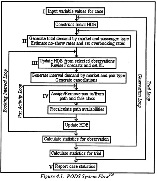
41 PODS Ssvtem Flow 74

PODS Inputs

Demand Generation by Market and Booking Interval Forecasting and Seat Inventory Control

Passenger Assignment / Cancellation 4.5.1. Boeing Decision Window Concept 4.5.2. The Passenger Activity Loop 4.2.

4.3. 4.4.

V. Description of Evaluated Methods and Simulation Environment 87

5.1. Base Case Simulative Environment 87

5.1.1. System-Level Inputs 87

5.1.2. Airline-Level Inputs 88

5.1.3. Market-Level Inputs and all Fare-Related Inputs 88

5.2. Forecasting Methods 91

5.2.1. Non-Causal Regression (Advance Bookings) 91

5.2.2. Classical Pickup (Historical Bookings) 94

5.2.3. Boeing Efficient Forecaster (Combined) 95

5.2.4. Conditions to be Tested 98

5.3. Detruncation Methods 98

5.3.1. No Detruncation 99

5.3.2. Booking Curve Detruncation 99

5.3.3. Projection Detruncation 101

5.3.4. Pickup Detruncation 103

5.3.5. Condition to be Tested 104

5.4. Sell-Up Models 104

5.4.1. Modify Booking Limits 105

5.4.2. Conditions to be Tested 105

VI. PODS Revenue Results 107

6.1. Forecasting Model Comparisons 107

6.1.1. Pickup/Regression Comparisons 107

6.1.2. Efficient/Pickup Comparisons 132

6.2. Detruncation Model Comparisons 142

6.2.1. Base Case and HighlLow Demand Factor Scenarios 142

6.2.2. High/Low Booking Curve Variability Scenarios 151

6.2.3. High/Low System K-Factor Scenarios 155

6.3. Sell-Up Analysis 159

6.3.1. Base Case and High Demand Factor Scenarios 161

6.3.2. High Price Sensitivity Scenarios 168

6.3.3. Booking Curve Scaling Scenarios 173

6.3.4. Additional Frequency Scenarios 177

VII. Summary and Future Directions 183

7.1. Synopsis of the Thesis 183

7.1.1. Definitions 183

7.1.2. Review of Past Comparative Studies and Models 184

7.1.3. Models Tested in the Thesis 184

7.2. Principal Findings 186 7.2.1. Forecasting Methods 186 7.2.2. Detruncation Methods 187 7.2.3. Sell-Up Analysis 188 7.3. Future Directions 190 Bibliography 192

List of Tables

2.1. Hypothetical Characteristics of a Request by Pax Type 28

2.2. Typical Airline Fare Structure 29

2.3. Percentage of Travelers Able to Meet Fare Restrictions, by Pax Type, Flights over 1300 Mi. 30

4.1. PODS System-Level Inputs 77

4.2. PODS Airline-Level Inputs 78

4.3. PODS Market-Level Inputs 78

5.1. PODS Base-Case Fare Structure 90

5.2. PODS Base-Case Passenger Type Details 90

6.1. Pickup versus Regression Forecasting Relative Revenue Performance 108

6.2. Loads for No Detruncation Scenarios 110

6.3. Loads for Booking Curve (No Scaling) Detruncation Scenarios 117

6.4. Loads for Booking Curve (DF = 1.2) Detruncation Scenarios, Variable Scaling 119 6.5. Loads for Booking Curve (DF = 0.9) Detruncation Scenarios, Variable Scaling 119

6.6. Loads for Pickup Detruncation Scenarios 121

6.7. Loads for Projection Detruncation Scenarios 124

6.8. Percentage Revenue Differences between Pickup and Regression under Variable 7f2 125 6.9. Loads with Variable zjf, Booking Curve detruncation, pbscl = 0.6 or 1.0, DF = 1.2 126 6.10. Percentage Revenue Difference under Variable System k-factor; DF = 0.9 129 6.11. Loads under Variable sf, Booking Curve Detruncation (pbscl = 1.0), DF = 0.9 130 6.12. Loads with Variable Scaling under Booking Curve Detruncation; skf= 0.5; DF = 0.9 131 6.13. Pickup versus Efficient Forecasting Relative Revenue Performance 133 6.14. Efficient and Pickup Loads with Variable DF, pbscl = 1.0 133

6.15. Efficient and Pickup Loads with Variable pbscl, DF = 1.2 135

6.16. Pickup versus Efficient Forecasting Relative Revenue Performance under Variable rf2 136 6.17. Efficient and Pickup Loads with Variable zf2, pbscl = 0.6 or 1.0, DF = 1.2 137 6.18. Pickup versus Efficient Forecasting Relative Revenue Performance under Variable skf, DF = 0.9 139 6.19. Efficient and Pickup Loads with Variable skf, pbscl = 0.6 or 1.0, DF = 0.9 141 6.20. Booking Curve (No Scaling) Versus Other Detruncators: Relative Revenue Performance at Several DF 143 6.21. Loads under Variable DF between Booking Curve (No Scaling) and No Detruncation 143 6.22. Closure Rates under Variable DF between Booking Curve (No Scaling) and No Detruncation 144

6.23. Three-Airline Variable Control Method Revenue Results 145

6.24. Loads under Variable DF and Scaling Levels for Booking Curve Detruncation 146 6.25. Loads under Variable DF between Booking Curve (No Scaling) and Projection Detruncation 149 6.26. Loads under Variable DF between Booking Curve (No Scaling) and Pickup Detruncation 150 6.27. Booking Curve (No Scaling) Versus Other Detruncators: Relative Revenue Performance at Several 7f2 154 6.28. Loads under Variable z2 between Bk Crv (No Scaling) and Bk Crv (pbscl = 0.6) Detruncation 155 6.29. Booking Curve (No Scaling) Versus Other Detruncators: Relative Revenue Performance at Several skf 156 6.30. Loads under Variable skf between Booking Curve (No Scaling) and No Detruncation, DF = 0.9 157 6.31. Closure Rates under Variable skf, Booking Curve (No Scaling) and No Detruncation, DF = 0.9 158

6.32. Sell-Up Objective Performance, Base Case 163

6.34. Sell-Up Objective Performance at Low ACR and Variable DF 169 6.35. Sell-Up Objective Performance under Variable pbscl, Base ACR, DF = 0.9 176 6.36. Sell-Up Objective Performance under Variable Airline A Frequency, Base ACR, DF = 0.9 178 6.37. Sell-Up Objective Performance under Variable Airline B Frequency, Base ACR, DF = 0.9 181

List of Figures

1.1. Nondiscretionary versus Discretionary Booking Curves 10

1.2. The Seat Inventory Control Process 11

1.3. Details of the Seat Inventory Control Process 14

1.4. Airline/Passenger Interaction, with Links to Seat Inventory Control 18

2.1. Basic Supply and Demand Graph 21

2.2. Declining Average Curve Above Marginal Cost Curve 23

2.3. Second Degree Price Discrimination with Declining Average Cost 25

2.4. Market Demand Segmentation Model 27

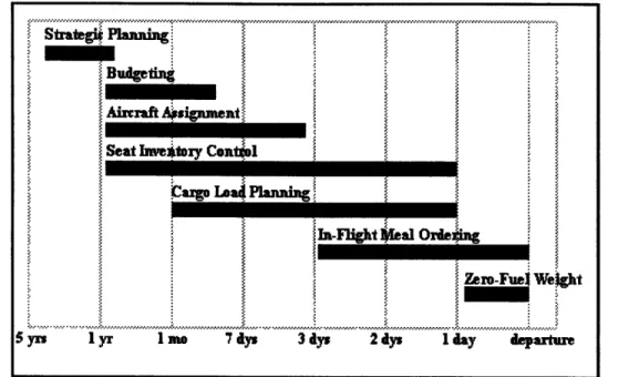
3.1. Ideal Flight-Specific Timeframes for Airline Forecasting Applications 36

3.2. Forecasting Techniques 37

3.3. Forecasting in the Seat Inventory Control Process 40

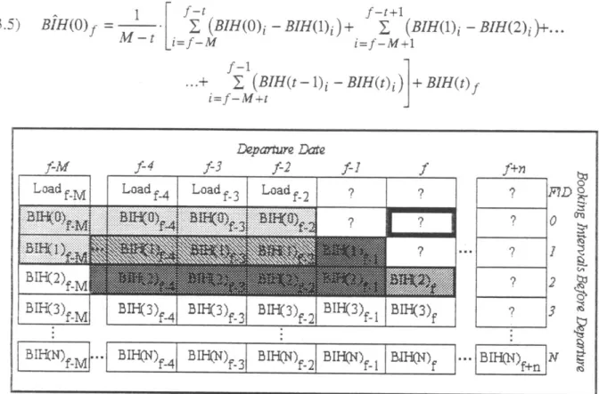
3.4. Booking Data Utilized in Historical Bookings Models 44

3.5. Bookings Data Utilized by Classical Pickup 45

3.6. Bookings Data Utilized by Advanced Pickup 46

3.7. Bookings Data Utilized in Advance Bookings Models 48

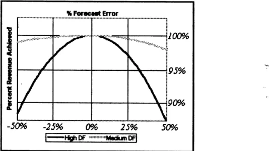
3.8. Revenue Losses as a Function of Forecast Error, High and Low Demands 54

3.9. Inherent Biases in Measurements of Forecast Error 55

3.10. Pickup Forecasting with Censored Flights 57

3.11. A Censored Demand Distribution 61

4.1. PODS System Flow 76

4.2. Recursive Nature of Seat Inventory Control 81

4.3. Schedule States for a Simple Market 83

4.4. Passenger Activity Loop 85

5.1. Representative Booking Curves 100

5.2. Projection Detruncation 102

6.1. Regression versus Pickup Forecasting Revenue results, by Detruncation method (DF = 0.9 and 1.2) 109

6.2. Samples Booking History 11l

6.3. Booking Correlation between Intervals and Range of Final Demand 112 6.4. Pickup versus Regression Forecasting-Treatment of Outliers 113

6.5. Booking Curve Detruncation 114

6.6. Effect on Regression Slope of an Additional Observation, by Region 116

6.7. Pickup Detruncation 121

6.8. Projection Detruncation for a Forecast Flight 122

6.9. Projection Detruncation 123

6.10. Revenue Performance for Variable r.2 by Airline and Detruncation Choice, DF = 1.2 128

6.11. Airline and Total Revenues under Variable skf 140

6.12. Percent Revenue Difference with Variable Scaling, Airline A over Airline B 148

6.13. Revenue Change over No Detruncation, DF = 0.9 152

6.14. Revenue Change over No Detruncation, DF = 1.2 153

6.15. Probability Distribution of Bookings under Moderate and High skf 157

6.16. Revenues with Increasing SU, DF = 0.9, Base ACR 162

6.17. Revenues with Increasing SU, DF = 0.9 and 1.2 164

6.18a. Airline A Total and Per-Class Loads, DF = 0.9, Base ACR, with Increasing SU 166 6.18b. Airline B Total and Per-Class Loads, DF = 0.9, Base ACR, with Increasing SU 166 6.19a. Airline A Total and Per-Class Loads, DF = 1.2, Base ACR, with Increasing SU 167 6.19b. Airline B Total and Per-Class Loads, DF = 1.2, Base ACR, with Increasing SU 167

6.20. Revenues with Increasing SU, Variable ACR, DF = 0.9 170

6.21. Revenues with Increasing SU, Variable ACR, DF = 1.2 171

6.22a. Airline A, B Single Revenues with Increasing SU, Variable Scaling; DF = 0.9, Base ACR 174 6.22b. Airline A, B Joint Revenues with Increasing SU, Variable Scaling; DF = 0.9, Base ACR 174 6.23. Loads under Joint Adjustment with Increasing SU, Variable Scaling; DF = 0.9, Base ACR 175 6.24a. Single Per-Flight Revenues with Increasing SU, Variable A Frequency 179 6.24b. Joint Per-Flight Revenues with Increasing SU, Variable A Frequency 179 6.25. Single Per-Flight Revenues with Increasing SU, Variable B Frequency 180

I. Introduction

1.1. A brief introduction to revenue management and forecasting 1.1.1. Why revenue manage?

Suppose that there are but two types of consumers who purchase a product. The first type values the product highly and so is willing to pay much more than the other type. This first type also values superior product characteristics and will pay more for them. Any sensible businessperson would try to segment the two, offer the appropriate level of services, and charge accordingly.

Airlines are no exception. The first problem of airline revenue management is to try to identify what passengers value, and how they fall into types ranked by willingness to pay (WTP).

If passengers all arrived at once, revenue management's task would simply be to identify whether

a passenger was high-value or not and then charge accordingly (this raises the issue of price discrimination, which I will address later). If a direct signal of WTP is unavailable, an airline could resort to measures that are closely correlated. One example would be how "discretionary" is the passenger's trip, i.e., how flexible an individual is making a reservation on this flight.

But passengers do not arrive at once. The booking process before a flight over which reservations may be made is up to a year in length. Neither discretionary nor nondiscretionary passengers make reservations randomly throughout the booking process. Instead, as shown in Figure 1.1, the greater proportion of discretionary bookings for a typical U.S. market are made

early in the process, while most nondiscretionary bookings are made shortly before departure.

This creates a vexing problem: If low-value passengers arrive early and high-value passengers late, how do we ensure that enough seats are saved for later-arriving passengers without unnecessarily turning away low-value early arrivals? Much thought and not a few careers are dedicated to finding the optimal solution to this, airline revenue management's second problem. The industry is continuously regaled by claimants who are sure they have found the

optimal revenue solution -- a seat optimization algorithm which strikes the correct, revenue

O 1 - --- ---2

8

Days Before Departure

"- nondiscretionary - -discretiona

Figure 1.1. Nondiscretionary versus Discretionary Booking Curves

As shown in Figure 1.1, the booking process is divided into N time intervals of unequal length (the duration of each interval decreases as the departure date nears). Between each interval, an updated forecast of final demand is made, usually based in part on actualized bookings until that point, and the seat optimization algorithm is rerun. A booking interval is thus defined as a length of time within the booking process in which passengers make reservations but no reoptimization occurs. A large number of intervals is computationally impractical, while too few allows no adjustment for differences between forecast and actual bookings as the booking history for that flight develops. For most U.S. carriers, N is typically 10-25.

Presently, airlines address the two revenue management problems by (1) offering several fare classes on a given flight, each with a different set of restrictions designed to target the fare product to the appropriate passenger type, and (2) using a seat optimization algorithm to appropriately limit the seats available to lower-valued fare classes. It is an involved and complex process, but worth the trouble: Revenue management has repeatedly been shown to yield significant revenue benefits over not offering different fare products at all, or offering different products without limiting availability using a seat optimization algorithm2_.

1.1.2. Where forecasting fits in

2 Actual trials of an early leg-based seat optimizer at Western Airlines are explored in Belobaba (1987); revenue

simulations of more advanced network and quasi-network optimizers are given in Williamson (1992), Tan (1994), and Ferea (1996). Leg-based revenue simulations utilizing PODS, a comprehensive simulator of the passenger demand generation and allocation process, are given in Wilson (1995).

The two processes of constructing fare products and limiting seats to lower-valued fare classes are not independent. As shown in a simplified, idealized diagram of the seat inventory control process (Figure 1.2), such procedures involve only steps 1b, 3, and 4 of the process. This description of seat inventory control is idealized: Some airlines will adopt additional procedures, while others will not complete all the steps described here.

J(la) Collection of HistoricalDataBase ) (1b) Construction of Fare Structurei

(2) Forecasting Procedures by Fare Class

(3) Seat Optimization Algorithm

(4) Setting of Booking Limits by Fare Class

I

(5a)Passenger Booking Process

.- - - Flight Day Loading Process i

Figure 1.2 The Seat Inventory Control Process

Between each interval in the booking process, Steps la through 4 are performed, except

Step lb. This step is represented with a dash because realignments to the existing fare structure (e.g., major fare changes, adjustment of the number and/or restrictions on fare products) are

performed less often and require extensive analysis of expected changes of the allocation of

bookings to each fare class under the new structure. Careful examination of historical booking

data under the existing fare structure provides clues about expected changes. Once these

expected changes have been estimated, the historical database is adjusted by the results of this analysis, which is then input into the forecaster. Step lb is usually considered to be a pricing

function; I include it in Figure 1.2 because of its extensive interaction with seat inventory control. Step 5b is dashed because it occurs only on flight day, after the booking process is complete. I will examine the seat inventory control process in more detail under Section 1.3.

Because seat optimization algorithms in Step 3 calculate allocations of seats between fare classes, their success depends upon forecasting tools used in Step 2, which give an accurate forecast of expected unconstrained demand by fare class for each leg3 _{or origin and destination} (O/D) pair the airline serves. The requirement of leg versus O/D forecasts depends on the

allocative level of the seat optimization algorithm: Most present optimization techniques allocate seats at the level of the leg4_{, but this is theoretically suboptimal to control on an O/D basis}5 because passenger travel itineraries may involve several legs. Regardless of the level of forecasting required, inaccurate forecasts result in distortions of seat allocations to fare classes, leading to suboptimal revenue performance.

Estimation of the Step 2 forecasts turns out to be a non-trivial problem itself, and there are many different methods to construct these inputs. It is curious but true that much less attention has been paid to the revenue effects of the different input methodologies than the seat optimization algorithms themselves. Presentations of novel seat optimization techniques routinely ignore difficulties in forecasting for their particular requirements, assuming instead that an accurate forecasting methodology is readily available.

1.2. Objective of Thesis

This thesis is an attempt to address the traditional neglect of forecasting and other input methodologies by testing their revenue effects in a competitive airline framework. I utilize a comprehensive simulation of the passenger demand generation and flow process originally developed by Boeing, called PODS (Passenger Origin and Destination Simulator). This simulator has several advantages which recommend it for realistically predicting revenue effects according to airline choices about input methodologies -- _{including barriers in the simulation between}

3 A "leg" is defined to be a flight stage involving one takeoff and one landing, or a nonstop flight.

SSee, _{e.g., the EMSRa algorithm developed in Belobaba (1987), or the EMSRb algorithm in Belobaba (1992).}

5

See Curry (1994) for an example of an O/D-based seat optimization scheme. Severe small number and run-time problems prevent actual use of O/D schemes at present.

forecasting methods and passenger generation processes, and a passenger choice framework which allows for realistic selection of airlines and flights under competition.

Besides testing the revenue effect of alternative forecasting models, I will use PODS to compare detruncation methods that adjust data from flights on which total demand is not known because booking limits set by the seat optimizer were reached. Without this step, the seat optimizer will not allocate enough seats to high-value passengers who could not book on historical flights because seats were already filled with low-value passengers. Finally, I will test

sell-up models which adjust for the willingness of some passengers to buy a more expensive fare

should their originally requested fare be unavailable.

1.3. The Seat Inventory Control Process

1.3.1. The Internal Airline Perspective

In this section I discuss the seat inventory control process in greater detail, first emphasizing the process which occurs internally at the airline, and then the parts of seat inventory control involving interaction between the airline and passengers. Close examination of the relationships between the processes I will test (ie., forecasting, detruncation, and sell-up) and seat inventory control provides a systematic understanding of the influences on these processes. Again, this depiction is idealized and does not describe the practice at any particular airline. Step

lb (governing changes in the fare class structure) will not be discussed.

The process begins at Step la in Figure 1.3, when previous departures of the flight to be forecast are initially selected from an airline's data on historical flights to form the Historical Data Base (HDB) for the forecast. Selection processes are designed to exclude previous flights which might have systematic differences with the flight in question. Thus, departures on different days of the week, with different aircraft sizes, or under differing competitive circumstances might be excluded from the data set.

The "unclean" data from the flights selected for inclusion are analyzed to remove and/or adjust entry errors, outliers, and other anomalous patterns in the data. Each previous flight in the database will have at least three characteristics: the total bookings BIH(O) received on each flight before the end of the last booking interval, which ends on the day of departure; no-shows (NS) who book but do not show up on departure day; and denied boardings (DB) -- would-be

passengers who book and show up but cannot board because of capacity restrictions on the aircraft . If there is strong seasonal variation over this dataset used for forecasting, it is adjusted to the season of the flight to be forecasted. Additionally, passenger loads are "detruncated" if previous load data are constrained by booking limits, ie., passenger loads in a fare class reach the limits established for that fare class at any time during the booking process.

Figure 1.3. Details of the Seat Inventory Control Process

After the data have been appropriately adjusted, bookings information goes into the

forecaster (Step 2). In the first booking interval (before any bookings on the flight have been

taken) the forecaster estimates expected unconstrained total bookings BIH(O)f or demand for the flight

f

In Step 4, information about NS and DB from previous flights, unadjusted booking limits provided by the seat optimizer, and the airline's estimation of the monetary cost of a denied boarding and no-show are analyzed by the overbooking model. It adjusts booking limits by trading off the expected benefit of accounting for no-shows with overbooking against the increased probability that more passengers will show up than space is available for.

Once adjusted booking limits BL for the ith interval have been provided by class, the booking process for the flight opens (Step 5a) and passengers may begin making reservations and (subsequently) cancellations. The seat availability SA or number of additional requests which will be accepted for each class is initially BLi. Once a passenger makes a reservation, SA on this fare class is decremented (BLi is set by the seat optimizer and therefore unchanged within booking intervals). Other fare classes' SA are also decremented. Many nested seat inventory control processes decrement SA in all higher-valued fare classes; others decrement SA in every fare class7. The rationale for the first policy is that the seat protection algorithm has already limited bookings in low-value classes via BL., given expected bookings in higher-valued classes. Decrementing SA in these classes therefore doubly impacts their availability -- once when BL are set, another when bookings are made in higher fare classes. At present, PODS decrements all fare classes. Because this approach decrements low value classes' SA more often, it closes low-value classes earlier.

This issue gives rise to a second measure of capacity on a fare class. For any given time within an interval i, I define the maximum allowable bookings Mx on a fare class to be the booking limit BLi established for that fare class, less net bookings received in i on other fare classes which affect this class' SA". Unlike BL but like SA, Mx reflects the fact that the maximum allowable bookings in a given fare class within an interval is continually adjusted for bookings made in other fare classes.

In any case, if after the reservation there is still space available in that fare class (SA > 0),

the fare class remains open for more reservations. If not (SA = 0), the fare class is closed, and no more reservations will be taken. However, if a passenger acts to cancel his or her reservation,

6 _{An interesting recent analysis of how best to do this is given by Holm (1995).}

7 Conceptually, these SA decrement strategies are heuristic compromises for the fact that adjustment of BL via reoptimization cannot feasibly occur after each booking/cancellation.

' Net bookings in these classes are total bookings less cancellations within interval i up until the time period of

interest. Generally, Mx * SA in a given fare class, because the latter includes bookings which occur during i within

seat availability is incremented (+ SA) and the fare class is opened again. The same booking limit

BLi for each fare class remains as long as the same booking interval (as discussed in Section 1.1

above) is in effect. When a booking interval ends and more intervals remain until departure, we

keep account of the total bookings-in-hand which have been received up to this interval i on this flight

f,

information provided by flights which have departed since the last run through the seat inventory control process. _{Then, the forecaster (Step 2) combines the revised information from the} historical data base with present bookings BIH(i)f to provide an updated forecast of total demand for the flight, by fare class9_{. The seat optimizer (Step 3) and overbooking models (Step 4) are} rerun, leading to booking limits BL,., for the (i-1)th interval0_{. Seat availability by class at the} start of interval i is then SA = BLi - BIH(i+J)f".

This process is repeated until no more booking intervals exist, i.e., flight day has arrived. On flight day, total bookings realized BIH(O)f for the flightf go into the HDB, and the passenger boarding process begins. Those passengers who do not show (NS) are recorded into the historical data base for this flight. Among those who do show up, if the overbooking model has correctly adjusted booking limits, there will be zero or few denied boardings (DB), which are also input into the HDB. Boarded passengers become passenger loads for this flight, which completes the HDB data set for this flight. The seat inventory control process for this flight is now complete.

1.3.2. The Airline/Passenger Interactional Perspective

Now I discuss a subsection of the seat inventory control process dealing with interaction between the passenger and airline. Steps 5a and 5b in Figure 1.3 above described the activity space over which passengers make requests for service, and airlines respond. Figure 1.4 expands these processes.

9 _{Instead of reestimating final demand during every reoptimization, some forecasters estimate the bookings to come}

from the present forecast interval until departure (see Section 5.2.1). 10

Many seat optimizers set booking limits on the basis of the remaining seats available on the flight. In this case, an estimate of bookings to come (BTC) would be necessary (see Footnote 9). BTC may be derived from forecasts

estimating final demands by the simple formula BTC = B/H(O)f -BIH(i)f. 1

1 It is therefore possible that SA < 0, if BIH(i+1) << BIH(i) and BL(i+1) >> BL(i) -- say, because of unexpectedly high bookings in high-value classes. In this case no bookings in the affected class are allowed in interval i unless many cancellations occur.

* Reservations Phase

When a potential passenger makes a request for a reservation on a particular O/D itinerary, either a travel agent (approximately 70 percent of the time) or an airline ticket/reservations agent (about 25 percent of the time) inquires the computerized reservations system (CRS) about space availability for the itinerary. A passenger can make a reservation in a particular class if seat availability SA is greater than zero, after all decrements and increments up to the present time. If so, a reservation is made and SA is decremented by one.

Otherwise, the potential passenger's initial request is denied, and (usually) an alternative will be offered. Those who accept the alternative -- either on the same flight in a more expensive fare class or on an alternative flight on the same airline -- are "recaptured" by the airline. Sell-up occurs in the former case (see Section 3.3), or if a potential passenger buys a more expensive fare product on an alternative flight. This behavior defines sell-up, but does not describe where adjusting for this possibility fits into the seat inventory control process. As I will show later in

Section 3.3, there are several methods to induce sell-up, each of which modifies a different part of the process. If the consumer refuses the offered alternatives and chooses a competitor or decides not to travel at all, the customer is lost to the airline.

e Confirmation Phase

One a passenger has made a reservation, he or she will receive a ticket upon appropriate payment to the airline. Before or after ticketing, the passenger may change plans and thereby

explicitly cancel the reservation, in which case seat availability SA for the fare class in which the

passenger was booked increase by one. The airline may also unilaterally cancel the reservation (resulting in an "implicit cancellation") if the passenger fails to meet some restriction associated with the ticket, e.g., purchase within one day of reservation (typical of low-value fare products) or reconfirmation of a reservation (typical on some international flights).

Figure 1.4. Airline/Passenger _{Interaction, With Links to Seat Inventory Ct}

* Boarding Phase

Finally, on the day of departure we enter the boarding phase, and the passenger can either show up for departure or may no-show, ie., not show up despite having a reservation and/or a ticket. No show probabilities are very specific to market and flight, and are generally higher on short-haul, high frequency, and business markets.

If the passenger does show up, space may not be available on the flight because of the overbooking. Airlines have established various procedures to compensate passengers denied

boarding -- _{i.e., those who arrive in expectation of traveling but find no seats available for them.}

After the flight has departed, total bookings received, loads, no-show and denied boarding

information are recorded to this flight's HDB, which will be later be used by the forecaster to predict total demand for future departures of the same flight.

1.4. Structure of Thesis

Chapter 2 provides a brief background of basic economic theory of supply and demand, and the types and profit potential of price discrimination. This chapter provides a theoretical explanation for the provision of multiple fare products with associated levels of restrictions. Whether or not airlines price discriminate is considered by examining current fare structures and their ability to "fence" passengers into desired groups. Finally, I discuss the arbitrary nature of this demand division for forecasting purposes.

Chapter 3 includes a theoretical motivation and review of the present literature on the three input methodologies this thesis focuses on: flight-level passenger forecasting, detruncation, and sell-up. I discuss models which have been advanced in the literature, and comparative studies using simulation or analysis of accuracy. Shortcomings of the various models and comparisons are discussed.

Chapter 4 gives a background in the architecture and theoretical assumptions used by

PODS, a simulator of passenger flow and revenues I use for comparing forecasting, detruncation,

and sell-up schemes. This chapter summarizes the salient points of PODS without extensive details, for which the reader is referred to Wilson (1995) -- the first installment of results from the joint MIT/Boeing collaborative research project on PODS. I also pinpoint some different

assumptions made by the PODS methodology and previous comparative studies of forecasters, detruncation methods, and sell-up mechanisms.

Chapter 5 describes the subset of models and methods from Chapter 3 I have chosen to compare using PODS. The assumptions and techniques of each of the tested methods are described. Chapter 6 is a discussion of simulation results for each of the chosen models and methods. Each comparison is run under a variety of conditions (e.g., demand conditions, demand stochasticity, frequencies in market, passenger characteristics) to examine the sensitivity of our conclusions about the revenue ranking of the described models to underlying market conditions. I present theoretical explanations of persistent revenue differences. These revenue results reinforce

the importance forecasting, detruncation, and sell-up play in determining the performance of the revenue management system.

Finally, Chapter 7 concludes with a detailed summary of these results and a short discussion of the projected future research areas for the Boeing/MIT PODS research project.

II. Revenue Management, Price Discrimination, and Product Differentiation

2.1.1. Basic Supply and Demand Theory

Basic neoclassical economic theory posits upward-sloping supply curves and downward-sloping demand curves in most markets". The latter results from the differential willingness to

pay property of the simple model of competitive markets: Some potential consumers are very

willing and able to purchase a product, but others are willing to purchase only if the price is lower. As price is successively lowered, more potential consumers are coaxed into purchasing the product. An opposite relationship obtains for producers: As more quantity is supplied, production costs rise as less efficient resources are employed to the production of the product. These relationships are depicted in Figure 2.1 where S(q) and D(q) represent the supply and demand curves, respectively.

PS

Ps

D(q)

.

SDq

Figure 2. 1, Basic Supply and Demand Graph.

" Hirschleifer and Glazer (1992), pp. 22-39 gives one of the innumerable treatments of supply and demand

relationships.

Under these conditions an equilibrium at point E results where the price consumers are willing to pay and the price suppliers are willing to accept is equal at Pe. Here Qe is exchanged. Any other quantity leads to a mismatch between the price consumers are willing to pay and the price suppliers are willing to accept. Negotiation between the two resolves the mismatch as price and quantity are driven to the equilibrium point.

With the uniform price Pe, some consumers are willing to pay more for the product but end up paying only Pe. For example, a customer Qi in Figure 2.1 is willing to pay up to Pi for the product but only pays Pe. This consumer gains consumer surplus in the amount Pi - Pe.

Analogously, the supplier gains a producer surplus of Pe - Ps from trade with the Qith consumer, because he or she would be willing to accept a price as low as Ps. The total surplus gained by consumers and suppliers as a result of exchange to Qe is represented by the shaded areas CS and

PS, respectively.

2.1.2. Disadvantages of Uniform Pricing

From the producer's perspective, uniform pricing has some disadvantages. Namely, CS remains to consumers as the benefit of this transaction. If market conditions and antitrust law permit, suppliers would prefer to obtain not only PS but CS. Under most market conditions a uniform price will always leave some surplus to consumers"1. Therefore, profits are not maximized.

Attempting to extract CS is commonly understood to be "bad" since it requires some consumers to pay more for the same product. There are three responses to this assertion. First, in an economic sense costless extraction of CS by producers is neutral. It does not affect the competitive equilibrium (Qe at price Pe in Figure 2.1), but is merely a transfer of funds from one to another economic actor. Second, when consumers have some degree of market power, quasi-monopsonistic conditions allow appropriation of the producer's PS -- but society rarely considers this to be a bad'.

"4 Tirole (1988), p. 133. Of course, consumers prefer the opposite: that they not only keep CS but extract PS from producers.

Third, under certain cost conditions, a producer cannot charge a single price and break even (let alone profit). Consider Figure 2.2, where demand D(q) is downward sloping as before but producer marginal cost (the cost of producing an additional unit) is constant, while average costs AC(q) (the total cost of production averaged over all units) are continuously declining. Such a situation would obtain if there were a high fixed cost to production and low costs of producing marginal units. In the airline industry, this is certainly true with respect to the provision of the marginal seat, where fixed costs include aircraft, gates, administrative, and other

16

expenses

Figure 2.2, Declining Average Curve above Marginal Cost Curve.

Under suppliers will

moderately competitive conditions and uniform pricing, economic theory posits that charge consumers the marginal cost of producing the good17_{. The supply curve}

16It is important to note that "fixed" versus "variable" distinction is defined only with respect to the time period

within which the decision to incur a particular cost is made. Thus, the aircraft fleet size decision is fixed within a decision period of a month, but variable within a year. For a sufficiently long time period (e.g., several years), all costs are variable, while all costs are fixed in the extremely short run. The time period of interest in this analysis is about a month, i.e., long enough for the individual flight decision to be variable while facilities and aircraft

available are fixed.

17 Hirschleifer and Glazer (1992), pp. 153-156.

Ci

Pi

S(q) is therefore equivalent to the horizontal marginal cost curve MC(q) in Figure 2.2. In this

illustrative case average costs are high relative to demand, so AC(q) is above D(q) for all q. Since under competitive uniform pricing the profit per unit for the producer is defined as average revenue (the uniform price) less average cost or S(q) -AC(q), the producer will always take a loss

regardless of production level q. At quantity

Qi,

A final argument against uniform pricing is the inefficiencies it creates by failing to account

for peak versus off-peak demand conditions. Economic theory indicates that when a good is not storable (e.g., electricity, which must be produced on demand), demand is subject to significant fluctuations, and provision of a unit of capacity is not free, uniform pricing will result in allocative distortions9. That is, in peak demand conditions individuals with the highest valuations of the good should receive the good while those with low valuations should purchase only in off-peak demand conditions. Under uniform pricing, each is just as likely to get the good. This is not a problem in off-peak periods because all can be accommodated. But in high periods some low-value individuals will receive the good, denying high-low-value individuals.

Peak load pricing avoids this by setting a higher price in peak periods and a low price in low periods. Only high-value consumers will be accommodated in the former, while all can be accommodated in the latter. Such pricing encourages the efficient use of resources as low-value consumers turned away in peak periods switch to off-peak consumption. This behavior is exhibited in the airline industry: A major point of studies of seat optimizers under variable demand conditions is the automatic protection of more seats for high fare passengers as market demand increases, thereby restricting availability of low fare seats to low demand flights20

2.2. Price Discrimination: An Alternative to Uniform Pricing

18 Hirschleifer and Glazer (1992), pp. 159-161.

1 Crew and Kleindorfer (1986), pp. 33-37; and Borenstein (1983), pp. 111-113.

20 See, e.g., Wilson (1995). Chapter 6 of this thesis will confirm these results. A significant benefit of seat optimization algorithms is the ability to identify and dynamically adjust to demand variations on a perflight basis as bookings develop. This is opposed to relying on generalizations about which seasons or days of week, etc. have high demand, and performing blanket adjustment of availability over presumably affected flights.

In certain circumstances, producers avoid the suboptimal condition of uniform pricing by

price discriminating -- charging different prices to different consumers for the same product. The

objective here is to somehow identify consumers by willingness to pay and charge accordingly,

and thus extract as much of the CS of Figure 2.1 as possible. Price discrimination is only operative if: it is legal2 , the producer/s can influence prices22 _{and can successfully identify} consumers by willingness to pay (WTP), and resale of product among consumers is impossible

(otherwise the identified low-WTP consumer buys all the product and resells to others).

Figure 2.3, Second Degree Price Discrimination with Declining Average Cost.

21 The Robertson-Patman Act prohibits some price discrimination, but it has never been applied to the airline industry. Several difficulties prevent such an application, including the understood exemption from the law of services and intangibles (Areeda [1981], p. 1058), the "like commodities" requirement that the products offered at varying prices be substantially similar, the cost differential by product defense (Areeda [1981], pp. 1102-1105), and the "meeting competition in good faith" defense (Areeda [1981], p. 1115). The recent antitrust lawsuits against airlines' pricing practices are a case in point. The allegations involved alleged price fixing attempts using CRS systems (Hunt [1994]). The Department of Justice did not raise a price discrimination issue, despite wide price ranges in fares which airlines allegedly attempted to fix.

22 _{This traditionally requires the market to be either monopolistic or oligopolistic. However, Borenstein (1983)}

shows that price discrimination can occur in reasonably competitive circumstances if products are somewhat heterogeneous between suppliers and consumers have brand preferences. A spatial model of monopolistic competition is used to prove this result.

Economists categorize methods of price discrimination into several types. Airlines are

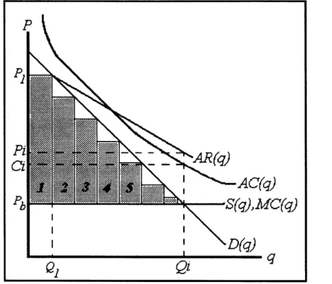
often accused of second-degree price discrimination, where a set of product "bundles" are offered. By voluntary market exchange, consumers choose the bundle most suited to them and incidentally forfeit more or less CS to the producer depending on their WTP. This type of price discrimination in the decreasing AC(q) with constant MC(q) case is shown in Figure 2.3. The producer has offered seven distinct products I ... 7 in decreasing order of price, and has successfully segregated consumers by decreasing WTP into the seven groups. Thus, consumers with the highest WTP purchase

Q,

Qj

purchase the product. At this production level the average cost per unit is Ci, which is above the demand curve D(q). However, because each of the seven groups of consumers have paid greater than the uniform price Pb at

Qi,

Qj)

Qi

average cost C. A profit per unit of Pi -Ci is earned. In this case price discrimination is preferred

by consumers and producers: It is the difference between the market existing or not. 2.3. The Discriminatory Nature of Airline Fare Structures

2.3.1. Identifying Passenger WTP and Type

Traditionally, airlines divided passengers into two types, business and leisure. Business travelers were assumed to have the higher WTP or, equivalently, lower price sensitivity. But consumer research in the late 1970s demonstrated that the distinction which should be drawn was between discretionary and nondiscretionary business travel, since some non-business travel is mandatory (e.g., emergencies among close relations), while some business travel is optional. Second, it was noted that passengers differ on variables other than simply price sensitivity: Some operate under extreme time constraints and others have more flexible schedules.

23 Tirole (1988), p. _135.

A two-axis representation of passenger type on price and time sensitivity variables was

developed by Belobaba25. As shown in Figure 2.4, this creates four types of passengers based on price and time sensitivity.

e Type I: Time-sensitive and price-insensitive. This category characterizes the nondiscretionary business traveler, especially one who is not personally paying for the trip. Such passengers have extremely tight schedules (requiring nonstop travel when possible), firm up travel plans very late, and often change plans. They are sometimes willing to pay for a superior cabin class. Type I business travelers dislike spending weekends out of town.

* Type II: Time-sensitive and price-sensitive. These passengers are nondiscretionary but are more concerned about price. They will not pay for first or business class and exhibit limited flexibility in schedules in order to obtain cheaper fares.

* Type III: Time-insensitive and price-sensitive. The typical leisure passenger falls into this group, which finds changes in travel date and even destination acceptable if it means a lower fare. Their schedule plans are typically set far in advance of travel.

e Type IV.: These few travelers have few constraints on travel dates, and are

willing to pay for superior service cabins and flexibility of travel arrangements in case they make alternative plans.

Low Price Sensitivi. High

High

III

I

0

" I IlI

Low .- - - .. - - -

-Figure 2.4. Market Demand Segmentation Model

Based on this information, the WTP ranking of the four passenger types is:

WTPJy WTP > WTPnJ WTP11. When a potential passenger makes a request for a reservation

as previously described (see Section 1.3 above), the request will contain information on at least the following characteristics listed below. If these variables signal underlying passenger type and associated WTP, tailoring specific products accordingly allows discrimination.

* Days before departure that request is made * One way or round trip

e If round trip, duration of stay at destination e If round trip, does stay involve a Saturday night * Desired time of departure/s or arrival/s

* Desired cabin of service

Table 2.1 provides hypothetical results by passenger type for each of the characteristics revealed by a potential passenger at time of request. Most characteristics appear to be good predictors of passenger type. Do airlines introduce different fares on these bases?

ypothetical Revealed Characteristics at Time of Request

Pax Days Until One Way or If RT, If RT, Departure/ Cabin of Type Departure Round Trip Duration of Saturday Arrival Time Service26

Stay Stay?

S < 7 OW <1 week No peak hours Y orC

II < 14 ? 5 1 week No more flexible Y

III > 14 RT > 1 week Yes very flexible Y

IV ? OW ? ? ? ForC

Table 2.1. Hypothetical Characteristics of a Request by Pax Type

2.3.2. Evidence of Possible Price Discrimination

An example of the array of fare classes offered on a hypothetical market is shown in Table 2.2 below. In this market, there are three cabins with varying levels of restrictions on each of the fare classes offered in the cabins. A "luxury" Type IV passenger will select to class C or F because of the superior service offered, the absence of restrictions, and full refundability of the product. Type I passengers, however, make reservations shortly in advance of travel, wish to spend weekends with family, and often travel for indeterminate lengths -- thus making round trip

2 These are standard cabin class (as opposed tofare class) distinctions: F is first class, C is business class, and Y is coach.

travel difficult. Combined with their desire to avoid to avoid the strict nonrefundability conditions of the low-valued classes, in these circumstances they will likely select a C, Y, or B fare.

Type II passengers are more flexible in timing arrangements but still dislike travel involving a Saturday, and sometimes change travel plans (thus making nonrefundability onerous, given their higher price sensitivity). They are likely to select a B, M, or (perhaps) an H fare. Finally, the typical leisure passenger is completely flexible with travel dates and Saturday night stays, and can make reservations far in advance. This type will therefore typically purchase the cheapest

Q

Airlines include fine gradations of fares within each fare class, -which sorts between the types of passengers who might select a particular fare class. For example, successively lower fares within the M fare class will be associated with more stringent restrictions on time of day, connections vs. one-way, and day of week to sort between the Types I and II passengers who typically purchase that fare class. The percentage proportion of the base Y-Class fare for each fare class is therefore an average over fares offered in that class. The illustrative example of Table 2.2 indicates significant price differences between and within cabin classes: A first class fare (F) costs five times the cheapest (Q) fare on the flight, while the most expensive coach class fare (Y) is about three times as expensive as the cheapest coach fare.

Fare Avg. Percent

Cabin Class of Y Fare Restrictions on Fare Class

First F 150% None (First Class)

Business C 120% None (Business Class)

Y 100% None (Full Fare Coach Class)

B 75% 3 Day Advance Purchase (A/P)

Coach M 60% 7 Day A/P, Sat. Night Stay

H 45% 14 Day A/P, Sat. Night Stay, Non Refundable, Round Trip

Q 30% 21 Day A/P, Sat. Night Stay, Non Refundable, Round Trip

Table 2.2: Typical Airline Fare Class Structure2 7

Limited information is available on how successfully these restrictions or "fences" direct passengers to the appropriate fare product. The complication involves an imprecise ability to identify a passenger's type from the information provided at time of request. The variables we

27 Adapted from Ferea (1996), p. 22 and Lee (1990), p. 30. Fare class structures vary slightly by airline and by market (only a limited number of markets have business class cabins, for example).

have examined are only imperfectly correlated with a passenger's willingness to pay, and some passengers will always be able to circumvent the designed sorting mechanisms by replanning their trip or other evasive methods". Thus, it is not possible to quantify the proportion of passengers

in each type.

A few independent attempts have been made at identifying the effectiveness of restrictions by passenger type. Results of a Boeing survey which asked passengers on markets of greater than 1,300 miles to classify themselves into one of three categories and then indicate whether they would on their present trip be able to meet a specified set of restrictions are given in Table 2.3 below29_{. The three categories -- nondiscretionary business (NDB), discretionary business, and}

leisure -- match fairly closely to Types I, II, and III, respectively.

Requirement % of Travelers Able to Meet Restriction, by

Type

Minimum Advance Non-Disc. Discretionary Leisure Total Stay Purchase Business Business

0 7 72% 86% 95% 86% 0 14 53% 77% 90% 76% 0 30 30% 61% 74% 59% 7 0 28% 32% 64% 48% 7 7 25% 28% 62% 45% 7 14 21% 27% 58% 41% 7 30 14% 23% 49% 34% Saturday 0 47% 56% 80% 66% Saturda 7 39% 51% 77% 61% Saturday 14 30% 47% 72% 55% Saturday 30 19% 40% 61% 45%

Table 2.3: Percentage of Travelers Able to Meet Fare Restrictions,

By Pax Type, Flights over 1300 Miles

While the restrictions considered are limited to a minimum stay and/or advance purchase requirement, the survey indicates that offering differing prices on these signals effectively fences passengers into appropriate fare classes: Only 28 percent of NDB travelers could accept a

seven-2 One common technique to avoid the Saturday night stay restriction is to buy two round trip tickets, one from

one's origin and the other from the destination, with scheduled departure dates on the first leg of each ticket matching one's original preferences. This is sensible only if the price of a Saturday stay round-trip ticket is less than half of the unrestricted price.

night stay restriction, while 64 percent of leisure travelers could. Similarly, the percentage of travelers able to meet advance purchase restrictions increases as we move from NDB to leisure, while declines as the restriction is tightened are more precipitous for NDB and discretionary business. Over the markets surveyed, the advance purchase restriction is most effective in screening between NDB and discretionary business, while the minimum stay requirement segments between business and leisure passengers. Table 2.3 in concert with Table 2.2 confirm the assertion that characteristics of the reservation request are important signals of differences in WTP3_{o, which airlines exploit by offering restricted fare products accordingly. That is, some}

evidence indicates that airlines offer different prices for substantially the "same" service. 2.3.3. Is Airline Behavior Actually Price Discrimination?

However, the arguments in Section 2.3.2 are absolutely not conclusive about whether or not airlines actually price discriminate. In this section I examine three arguments that the pricing structure in current practice is not discrimination at all. The primary point is that the various fares offered to passengers are not similar. If the fare products airlines offer are not the same, the evidence in Section 2.3.2 indicates only acceptable differential pricing.

First, consider the fact that potential passengers do not make requests for service at the same time. Some requests arrive early, others arrive late. If airlines adopted a first-come-first-serve strategy in that late arrivals would simply be denied service, it is justifiable that all be charged the same price. However, recognizing that many passengers cannot make decisions until late in the decision process, airlines save space for late-arriving passengers -- often explicitly turning away earlier-arriving passengers to do so. The result of this, of course, is a different price. Those arriving late also pay for having space saved for them until just before the flight. Early arrivals should pay less because there is a minimal likelihood that the airline has had to turn someone else away in order to serve them. The entire purpose of seat optimization schemes, as has been noted, is to strike the correct balance between saving enough seats for the uncertain 30 There are two caveats to Table 2.3. First, it is self-reported and therefore are subject to all the problems of surveys (e.g., correct interpretation of questions, class misidentification, and the stated versus revealed preferences problem). Second, the percentages are a function of fare differences between fare products assumed by respondents and the characteristics of the markets surveyed (e.g., a short-haul market will be more significantly affected by advance purchase restrictions).