A geodynamic model of mantle density heterogeneity
Texte intégral
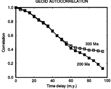
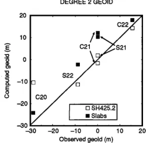
Figure
Documents relatifs
La prothèse totale chez le patient jeune comporte un certain nombre de difficultés. La première tient aux diagnostics responsables qui entraînent des anomalies
Nevertheless, high expression of Reg3β occurs in healthy pancreatic acinar cells surrounding the tumor, being this distant microenvironment the major source of Reg3β in
Along with the increased area used in the winding window, the higher turns ratio transformers increase the charge time as shown in Equation 3.14, or increase the primary peak current
— As a complément to data reported in an earlier note, the embryonic development of Scaeurgus unicirrhus (Orbigny, 1840) is described and discussed with spécial
Dube used THIOD and THERMIT-3 (THERMIT-3 refers to THERMIT with point kinetics) to perform two groups of reactivity feedback analyses. The first group consisted of
Dans notre cas, nous avons mesuré le temps que passe la souris dans un compartiment qui a été préalablement associé à un stimulus artificiel, le décageage de glutamate,
L’incompatibilité fœto-maternelle érythrocytaire RH1, constitue après l’IFM ABO, la principale cause d'anémie fœtale et d’anémie hémolytique chez les
In this paper, we present a measurement study to bring forth wireless network management issues faced during incremental Wi-Fi deployment on a university campus network.. We
