Scaling net ecosystem production and net biome production over a heterogeneous region in the western United States

(1)

HAL Id: hal-00297883

https://hal.archives-ouvertes.fr/hal-00297883

Submitted on 5 Apr 2007

HAL is a multi-disciplinary open access

archive for the deposit and dissemination of sci-entific research documents, whether they are pub-lished or not. The documents may come from teaching and research institutions in France or abroad, or from public or private research centers.

L’archive ouverte pluridisciplinaire HAL, est destinée au dépôt et à la diffusion de documents scientifiques de niveau recherche, publiés ou non, émanant des établissements d’enseignement et de recherche français ou étrangers, des laboratoires publics ou privés.

Scaling net ecosystem production and net biome

production over a heterogeneous region in the western

United States

D. P. Turner, W. D. Ritts, B. E. Law, W. B. Cohen, Z. Yang, T. Hudiburg, J.

L. Campbell, M. Duane

To cite this version:

D. P. Turner, W. D. Ritts, B. E. Law, W. B. Cohen, Z. Yang, et al.. Scaling net ecosystem production and net biome production over a heterogeneous region in the western United States. Biogeosciences Discussions, European Geosciences Union, 2007, 4 (2), pp.1093-1135. �hal-00297883�

(2)

BGD

4, 1093–1135, 2007

Scaling NEP and NBP in the western U.S.

D. P. Turner et al. Title Page Abstract Introduction Conclusions References Tables Figures ◭ ◮ ◭ ◮ Back Close

Full Screen / Esc

Printer-friendly Version Interactive Discussion

EGU Biogeosciences Discuss., 4, 1093–1135, 2007

www.biogeosciences-discuss.net/4/1093/2007/ © Author(s) 2007. This work is licensed

under a Creative Commons License.

Biogeosciences Discussions

Biogeosciences Discussions is the access reviewed discussion forum of Biogeosciences

Scaling net ecosystem production and net

biome production over a heterogeneous

region in the western United States

D. P. Turner1, W. D. Ritts1, B. E. Law1, W. B. Cohen2, Z. Yang1, T. Hudiburg1, J. L. Campbell1, and M. Duane1

1

Forest Science Department, Oregon State University, Corvallis OR 97331, USA

2

USDA Forest Service, PNW Station, Corvallis OR 97331, USA

Received: 22 March 2007 – Accepted: 27 March 2007 – Published: 5 April 2007 Correspondence to: D. P. Turner (david.turner@oregonstate.edu)

(3)

BGD

4, 1093–1135, 2007

Full Screen / Esc

EGU

Abstract

Bottom-up scaling of net ecosystem production (NEP) and net biome production (NBP) was used to generate a carbon budget for a large heterogeneous region (the state of Oregon, 2.5×105km2) in the western United States. Landsat resolution (30 m) re-mote sensing provided the basis for mapping land cover and disturbance history, thus

5

allowing us to account for all major fire and logging events over the last 30 years. For NEP, a 23-year record (1980–2002) of distributed meteorology (1 km resolution) at the daily time step was used to drive a process-based carbon cycle model (Biome-BGC). For NBP, fire emissions were computed from remote sensing based estimates of area burned and our mapped biomass estimates. Our estimates for the contribution

10

of logging and crop harvest removals to NBP were from the model simulations and were checked against public records of forest and crop harvesting. The predominately forested ecoregions within our study region had the highest NEP sinks, with ecore-gion averages up to 197 gC m−2yr−1. Agricultural ecoregions were also NEP sinks, reflecting the imbalance of NPP and decomposition of crop residues. For the period

15

1996–2000, mean NEP for the study area was 17.0 TgC yr−1, with strong interannual variation (SD of 10.6). The sum of forest harvest removals, crop removals, and di-rect fire emissions amounted to 63% of NEP, leaving a mean NBP of 6.1 TgC yr−1. Carbon sequestration was predominantly on public forestland, where the harvest rate has fallen dramatically in the recent years. Comparison of simulation results with

esti-20

mates of carbon stocks, and changes in carbon stocks, based on forest inventory data showed generally good agreement. The carbon sequestered as NBP, plus accumula-tion of forest products in slow turnover pools, offset 51% of the annual emissions of fossil fuel CO2 for the state. State-level NBP dropped below zero in 2002 because of the combination of a dry climate year and a large (200 000 ha) fire. These results

25

highlight the strong influence of land management and interannual variation in climate on the terrestrial carbon flux in the temperate zone.

(4)

BGD

4, 1093–1135, 2007

Full Screen / Esc

EGU

1 Introduction

Efforts to locate and explain the large terrestrial carbon sinks inferred from inversion studies (Baker et al., 2006; Bousquet et al., 2000) are faced with accounting for spa-tially extensive factors like climate variation and CO₂increase (Schimel et al., 2000), fine scale phenomena associated with anthropogenic and natural disturbances

(Ko-5

rner, 2003; Pacala et al., 2001), and temporal variation at the seasonal and interannual scales. Carbon budget approaches based on forest inventory information, e.g. Kauppi et al. (1992) are poorly resolved spatially and temporally, do not reveal the mecha-nisms accounting for changes in carbon stocks, and miss carbon flux associated with non-forest vegetation. Alternatively, a process modeling approach – with inputs of high

10

spatial resolution remote sensing data and distributed meteorological data - can pro-vide estimates of net ecosystem production (NEP, sensu Lovett et al., 2006) for poten-tial comparison with NEP fluxes from inverse modeling studies, and provide estimates of net biome production (NBP, sensu Schulze et al., 2000) for comparison with carbon accounting being done in support of the Framework Convention on Climate Change

15

(UNFCCC, 1992). In this analysis, we apply a process modeling approach to generate a carbon budget over the state of Oregon (2.5×105km2) in western North America be-tween 1980 and 2002. The period included a significant reduction in forest harvesting on public lands, several extreme climate years, and an exceptional fire year.

The forests of the Pacific Northwest region of the United States (U.S.) are of

partic-20

ular interest with regard to terrestrial carbon flux because of their high biomass and productivity (Smithwick et al., 2003; Waring and Franklin, 1979), the mixture of land ownerships with differing management objectives (Garman et al., 1999), the sensitivity of the forest carbon balance to interannual climate variation (Morgenstern et al., 2004; Paw U et al., 2004), and potential for increased incidence of stand replacing fires in

as-25

sociation with projected climate change (Bachelet et al., 2001; Westerling et al., 2006). Earlier studies of carbon stocks and fluxes on forestlands in the region suggest that it is transitioning from a carbon source to a carbon sink (Cohen et al., 1996; Law et al.,

(5)

BGD

4, 1093–1135, 2007

Full Screen / Esc

EGU 2004; Wallin et al., 2007). Carbon flux in nonforest ecosystems of the region is less

well studied. However, the high productivities and large carbon transfers at the time of harvest in agricultural areas, and the large areas of semi-natural vegetation cover, could potentially have strong influences on the regional carbon budget.

2 Methods

5

2.1 Overview

The primary NEP/NBP scaling tool in this analysis was the Biome-BGC model (Thorn-ton et al., 2002) and details of its application for the purposes of scaling carbon pools and flux are given in previous publications (Law et al., 2004; Law et al., 2006; Turner et al., 2004; Turner et al., 2003). Generally, we used model simulations to produce

10

spatially-explicit estimates of carbon stocks as well as estimates of annual net primary production (NPP), heterotrophic respiration (Rh), and net ecosystem production for

each year from 1980 to 2002 over the state of Oregon. Annual NBP (NEP – harvest removals – pyrogenic emissions) was estimated from the simulated logging removals, crop harvest removals, and fire emissions. In our previous studies, we assumed all

15

forest stands originated as a clear-cut of a secondary forests, but in this application we introduced the capacity to simulate one or two clear-cut or fire disturbances (based on remote sensing) as the simulation for a given grid cell is brought up to 2002 after model spin-up. We have also begun modeling all vegetation cover types, thus permitting wall-to-wall estimation of the carbon pools and fluxes.

20

2.2 Land cover

We first established a forest/nonforest coverage based on areas analyzed in our pre-vious change detection studies (Law et al., 2004; Lennartz, 2005) Within the forest class, forest type was originally designated as evergreen conifer, deciduous broadleaf,

(6)

BGD

4, 1093–1135, 2007

Full Screen / Esc

EGU or mixed. However, we reclassified mixed as conifer here because a mixed class was

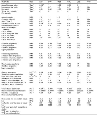
not supported in the Biome-BGC process model. We next overlaid a Juniper Woodland coverage from the Oregon GAP Analysis (Kagan et al., 1999). Lastly, we filled in all nonforest areas with the National Land Cover Data (NLCD) coverage (Vogelmann et al., 2001). These coverages were all based on Landsat imagery at the 30 m resolution.

5

The Transitional Vegetation Class in the NLCD coverage, which is primarily regrowing clear-cuts, was reclassified as conifer forest. Other NLCD classes were aggregated to a simple 7 class scheme (Fig. 1). The final coverage was resampled to the 25 m reso-lution for ease of overlay with the 1 km resoreso-lution climate data. Ecoregions boundaries are from the scheme of Omernik (1987).

10

2.3 Forest stand age and disturbance history

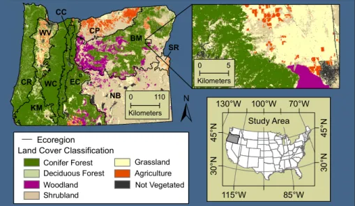
For each 25 m grid cell classified as forest, a disturbance history was formulated. These disturbance histories consisted of one or two disturbance events that were specified by year and type (fire or clear-cut harvest). Disturbances during the Landsat era (1972– 2002) were mapped (Table 1, Fig. 2) using change detection based on wall-to-wall

15

Landsat imagery every 2 to 5 years (Cohen et al., 2002; Healey et al., 2005; Lennartz, 2005). In our simulations, the disturbances were scheduled at the midpoint of each in-terval. Accuracy assessment of the stand replacement maps was conducted in Cohen et al. (2002) and reported as 88%. Assumptions about what was present at the time of the first disturbance were ecoregion specific, e.g. in the Coast Range ecoregion the

20

stand was assumed to be 75 years old to reflect the rotation age and the fact that much of the Coast Range had been harvested previous to the Landsat era (Garman et al., 1999).

For all conifer forestland in western Oregon that had no stand replacing disturbances during the Landsat era, stands were aged by classification into broad age classes

25

(young, mature, old) using recent Landsat imagery (as in Cohen et al., 1995). The ap-proach depends on spectral variation among stands of different ages associated with changes in stand structure. In eastern Oregon, it was not possible to age undisturbed

(7)

BGD

4, 1093–1135, 2007

Full Screen / Esc

EGU stands using Landsat data because the stands are relatively open and often uneven

aged. Thus for the ecoregions in the eastern part of the state, all conifer pixels >30 years of age were assigned the ecoregion specific, basal-area-weighted, median age (Waddell and Hiserote, 2005) from USDA Forest Service Forest Inventory and Anal-ysis data (FIA, 2006). Our previous chronosequence studies (Campbell et al., 2004)

5

in eastern Oregon have indicated that NEP remains positive over the course of mid and late succession in these relatively open stands, thus minimizing the error in NEP introduced by these assumed ages. As a sensitivity check, simulated NEP at a repre-sentative site and at the median age for each of these ecoregions was compared with the associated age-weighted mean NEP from Biome-BGC simulations based on the

10

age distribution of all FIA permanent plots in the ecoregion. Results did not indicate a strong bias (Table 2).

The deciduous broadleaf and mixed (reclassified as conifer) classes were assigned an age of 40, reflecting limited information from inventory data and knowledge from the change detection analysis that these stands were >30 years old. Juniper

wood-15

lands were assigned an age of 70 based on the observation that many of these stands have originated since the late 1800s when heavy grazing and fire suppression began to promote juniper expansion in eastern Oregon (Gedney et al., 1999). As with the open conifer stands in eastern Oregon, these woodland stands apparently continue to accumulate stem carbon over long periods (Azuma et al., 2005) which helps minimize

20

the error in estimating NEP. 2.4 Climate and soil inputs

The meteorological inputs to Biome-BGC are daily minimum and maximum temper-ature, precipitation, humidity, and solar radiation. We used a 23-year (1980–2002) time series at 1 km resolution developed with the DAYMET model (DAYMET, 2006;

25

Hasenauer et al., 2003; Thornton et al., 2000; Thornton and Running, 1999; Thornton et al., 1997). These data were based on interpolations of meteorological station ob-servations using a digital elevation model and general meteorological principles. The

(8)

BGD

4, 1093–1135, 2007

Full Screen / Esc

EGU 23-year record was recycled as needed during the model spin-ups. Soil texture and

depth were specified (at the 1 km spatial resolution) from the U.S. Geological Survey coverages (CONUS, 2007) that were originally generated by linking soil survey maps of taxonomic types to soil pedon databases (Miller and White, 1998).

2.5 Biome-BGC parameterization and application

5

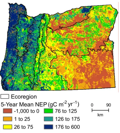
The parameterization of ecophysiological and allometric constants in Biome-BGC (Ta-ble A1) was cover type and ecoregion specific. The values used were based on the literature (e.g. Pietsch et al., 2005; White et al., 2000), our field measurements (Law et al., 2004; Law et al., 2006), and our previous work with the model in this region (Turner et al., 2003, Law et al., 2004). Our field measurements (extensive plots) included over

10

100 plots in the study region that were distributed so as to sample the range of age classes within the conifer cover class in each ecoregion. The foliar nitrogen concentra-tion and specific leaf area (SLA) measurements from these plots were used to specify foliar C to N ratio and SLA in the conifer class (Table 3). Earlier sensitivity analyses with Biome-BGC (White et al., 2000; Tatarinov and Cienciala, 2006), have revealed

15

that the model is particularly sensitive to these parameters. Recent studies support the utilization of ecoregion-level reference data for model parameterization when it is available (Loveland and Merchant, 2004; Ogle et al., 2006).

As noted in Law et al. (2004), we have adapted Biome-BGC so that input parameters can be dynamic over the course of forest succession. Previously we used this feature

20

to shift production belowground in late succession to reflect the age trends in bolewood production that are observed in FIA data (Law et al., 2006). Here, we have also made the mortality fraction a dynamic parameter (see Pietsch and Hasenauer, 2006) such that mortality may decrease over the course of succession. The range of mortality was made consistent with studies in the region (Acker et al., 2002; DeBell and Franklin,

25

1987; Lutz and Halpern, 2006). This feature was needed for simulating the forests of eastern Oregon which show sustained increases in biomass even in late succession (Campbell et al., 2004; Van Tuyl et al., 2005). Another modification to Biome-BGC was

(9)

BGD

4, 1093–1135, 2007

Full Screen / Esc

EGU to constrain the maximum daily interception, as discussed in Lagergren et al. (2006).

For a standard model run, the model was spun-up and run forward through the sim-ulated disturbances to the year 2002, with looping of the 23 years of climate data as needed. For non-forest, non-woodland cover types, the model was spun-up and run to near carbon steady state by 1980 so that its year-to-year variation in NEP primarily

re-5

flected the influence of climate variation. In the case of croplands and grasslands (hay-fields), where carbon is removed in the form of harvesting, we included the removals in the Biome-BGC simulations as we ran up to the present, thus the NEP tended to balance the removals (i.e. these areas are carbon sinks in terms of NEP).

Because of the computational demands of the model spin-ups, it was impractical

10

do an individual model run for each 25 m resolution grid cell in the study area. The 1 km resolution of the climate data is adequate to capture the effects of the major climatic gradients, but our earlier studies in this region have shown that the scale of the spatial heterogeneity associated with land management is significantly less that 1 km (Turner et al., 2000). Thus, the model was run once in each 1 km cell for each of

15

the 5 most common combinations of cover type and disturbance history. For mapping the carbon fluxes, a weighted mean value was calculated for each 1 km cell. This procedure explicitly accounted for 97% of the study area.

2.6 Harvest removals and fire emissions for NBP estimation

Estimation of NBP requires information on carbon transfers off the land base in addition

20

to NEP (Schulze et al., 2000). To quantify wood harvest removals we assumed that 65% of wood carbon was removed at the time of harvest (Turner et al., 1995). For a check on our simulated harvest removals, these values were summed to the state level and compared with harvest data from the Oregon Department of Forestry (ODF, 2006). The ODF volume data were converted to carbon mass using the carbon densities in

25

Turner et al. (1995). For the year-specific NBP calculations, we partitioned the total simulated removals among the years in a given change detection interval by reference to the partitioning in the ODF volume data.

(10)

BGD

4, 1093–1135, 2007

Full Screen / Esc

EGU Crop removals must also be quantified for NBP and here we assumed 80% of

above-ground biomass was removed annually on all cropland and grassland grid cells. This crop ratio approximates the crop ratios in U.S. Department of Agriculture National Agri-cultural Statistics Service (NASS) reports for Oregon (USDA, 2001).

Direct emissions from forest fire can be a large term in NBP estimates and here

5

were based on the change detection analyses for area burned, on carbon stocks in the burned areas from the Biome-BGC modeling, and on transfer coefficients that quanti-fied the proportion of each carbon stock that burned. We assumed 100% of foliar, fine root, and litter carbon was emitted, and 7% of aboveground wood. These values are similar to those found in high burn severity areas of a large wildfire in our study area

10

(Campbell et al., 20071). The remainder of the wood was transferred to the coarse woody debris pool. Again, for the year-specific NBP calculations we partitioned the di-rect fire flux among the years of the change detection interval by reference to the ratio of area burned in a given year to area burned over the interval from state-level burned area statistics (NWCC, 2004).

15

2.7 Uncertainty assessment

Estimates of carbon stocks are important in the simulation of harvest removals and fire emissions, as well as giving a general indication of model behavior. For an inde-pendent estimate of the regional carbon stocks on forest land, USDA Forest Service inventory data (8929 plots in Oregon) can be summarized at the county level. Allometry

20

and carbon density factors are used to convert volumes to total tree carbon and refer-ence is made to expansion factors associated with the plot-level data to account for the sampling scheme (Hicke et al., 2007). The uncertainty associated with inventory-based bolewood volume estimates over large areas such as counties in the U.S. is considered to be less than five percent (Alerich et al., 2004). Uncertainty about the allometry used

25

1

Campbell, J. L., Law, B. E., and Donato D: Carbon emissions from the Biscuit Fire, J.Geophys. Res. - Biogeosci., in review, 2007.

(11)

BGD

4, 1093–1135, 2007

Full Screen / Esc

EGU to scale volume to biomass is also relatively low (Van Tuyl et al., 2005). For comparable

values from our Biome-BGC simulations, we averaged simulated tree biomass (wood-mass) in 1995 (the end of the last inventory cycle) over all forested areas within each county. For other cover types, limited comparisons were made between the simulated carbon stocks and observations in the literature.

5

Evaluation of carbon flux on forestland, at least in terms of tree NBP, can also be made based on forest inventory data. Aggregated inventory data in the U.S. are peri-odically reported in terms of cubic feet of bolewood volume per unit area (Smith et al., 2004) and NBP (for trees) can be estimated as the change in total stocks divided by the associated interval. For our comparisons we used a conversion factor of 6.4 kgC per

10

cubic foot and a ratio of tree carbon to bolewood carbon of 1.7 (Turner et al., 1995). For NEP, we have previously reported comparisons of our Biome-BGC simulations to field measurements at an eddy covariance flux tower and at chronosequence plots in the region (Law et al., 2004; Law et al., 2006). For cropland/grassland NPP and harvest removals, we made comparisons to USDA NASS statistics (USDA 2001) aggregated

15

to the ecoregion scale.

It was not feasible to perform a formal uncertainty analysis for inputs and parame-ters of our state wide NEP simulations (e.g. using a Monte Carlo approach at each point and summing uncertainty across the domain) because of computational con-straints, because we don’t know the moments and distribution types for the multitude

20

of parameters in Biome-BGC, and because the error sources are not spatially inde-pendent. However, it is worth noting that the NEP estimates for forestland are to some degree stabilized against model parameter values affecting rates of growth (carbon sinks) because high growth rates create relatively large carbon stocks which become large carbon sources when disturbed. Similarly, artificially high rates of decomposition

25

would push up carbon sources in the short term after disturbance but, since the model maintains mass balance, the total amount of heterotrophic respiration would tend to be similar over a whole successional cycle even with lower base turnover rates for Rh.

(12)

BGD

4, 1093–1135, 2007

Full Screen / Esc

EGU available as the density of CO₂ measurements supporting inverse modeling efforts

increases (Karstens et al., 2006). Here, we made a first order comparison with opti-mized terrestrial carbon flux estimates over Oregon from the Carbon Tracker inversion scheme (NOAA, 2007).

3 Results and discussion

5

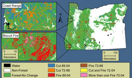
3.1 Five-Year mean flux estimates

For assessing the recent carbon budget we report means and standard deviations (over years) for the 5-year period 1996–2000 (Table 4). This period was after harvest levels stabilized following the significant decrease in the early 1990s (Fig. 4) and before the relatively warm/dry climate years of 2001 and 2002 (2002 was the driest of the 23 year

10

record). Over that interval, the Oregon land base was a strong NEP sink, with total NEP averaging 17.0±10.6 TgC yr−1 (67±42 gC m−2yr−1).

Our statewide NEP estimates contrast with those from approaches that do not ex-plicitly treat the disturbance regime. Prognostic models that are simply spun-up and run forward on historical climate report a smaller NEP sink in the region, e.g.

averag-15

ing about 30 gC m−2yr−1 in the 1990s in the study of Woodward et al. (2001). The carbon sink in that simulation was driven by a small disequilibrium in the carbon pools associated with the increasing CO₂concentration. Diagnostic models, driven by con-temporary observations of climate and surface greenness from remote sensing, show Oregon as a carbon source over the period 1982–1997 (Potter et al., 2006), probably

20

because of a warming trend (Mote, 2003).

The Coast Range and West Cascades ecoregions both had high mean NEP (Fig. 4, Table 5), but for different reasons. Forest productivity in the Coast Range is high be-cause of the mild, mesic climate, and bebe-cause intensive forest management for timber production has resulted in a relatively young age distribution at this time (Van Tuyl et

25

(13)

BGD

4, 1093–1135, 2007

Full Screen / Esc

EGU NPP at a given age is somewhat lower in the West Cascades ecoregion than in the

Coast Range (Gholz, 1982). However, harvesting on public lands in Oregon (69% of the forested land in the West Cascades ecoregion) was extensive in the decades lead-ing up to the 1990s but has subsequently been restricted due to issues associated with the Northwest Forest Plan (Moeur et al., 2005). Much of the area harvested earlier

5

is now a carbon sink and there is relatively little area on public lands that is a car-bon source because of recent harvesting. The forests in eastern Oregon (EC and BM ecoregions) were a weak carbon sink from NEP, the net effect of relatively low NPP and NEP in a large area of undisturbed stands in a relatively xeric climate, and strong emissions in the areas subject to fire or harvest. In recent years, the proportion of

10

forestland disturbed per year (harvest or fire) in eastern OR has been greater than for western OR (Table 1), which helps explain the weaker carbon sink there.

The highest NEPs in ecoregions that are not heavily forested were in the agricul-tural zones of the Willamette Valley and Columbia Plateau ecoregions (Fig. 4, Table 5). There, large areas are planted with highly productive grass or winter wheat, thus

gen-15

erating a high NPP. The heterotrophic respiration in cropland areas is generally much less than NPP (Table 6) because much of the biomass is removed and only residues are plowed back into the soil to decompose (Anthoni et al., 2004; Moureaux et al., 2006).

The large area of Juniper woodlands in eastern OR (Fig. 1) had a low positive mean

20

NEP (41±56 gC m−2yr−1) reflecting slow accumulation of bolewood carbon. Earlier studies have highlighted the potential carbon sink from widespread expansion of land in the western US over the last century (Houghton et al., 1999). The total wood-land NEP for Oregon averaged 0.6 TgC yr−1over the reverence interval.

The NEP for the large area of shrubland in SE Oregon was slightly negative (–

25

10± 46 gC m−2yr−1) but with interannual variation that included years of positive NEP. The large area of shrubland brought the total for this source to –0.7 TgC yr−1 between 1996 and 2000. This carbon source was the product of a drying trend over the refer-ence period and is consistent with recent eddy flux measurements in a mature

(14)

sage-BGD

4, 1093–1135, 2007

Full Screen / Esc

EGU brush community in the western U.S. (Obrist et al., 2003).

NBP for the study region was 6.1±10.2 TgC yr−1over the 1996–2000 period. Of the ecoregions where NBP was positive, the highest ratio of NBP to NEP was in the Cas-cade Crest ecoregion (Table 7). This is a high elevation ecoregion where there is little logging or fire. Lower NBP to NEP ratios were found in areas subject to more

inten-5

sive management. Our simulated timber harvest removals were 5.9±0.3 TgC yr−1 and were predominantly from the highly productive privately owned forest lands in western Oregon. Harvest removals associated with agricultural lands and grasslands were of a lower magnitude 4.8±0.3 TgC yr−1, but made a significant contribution to the total harvest flux. The contribution of cropland/grassland to NBP was small (–0.3 TgC yr−1)

10

because harvest removals approximately balanced NEP for these lands. Direct carbon emissions from wildfire averaged 0.2 TgC yr−1, which is small relative to forest NEP and harvest removals. Overall, the predominant source of positive NBP was forestland and the high interannual variation in NBP during the reference years was primarily a function of interannual variation in NEP.

15

The regional total for NBP in Oregon masked a strong difference between the fluxes on public and private forestland. In our analysis, the majority of the forestland NBP for the state was associated with public lands. On private lands, the ratio of growth to removals is close to one (Campbell et al., 2004; Alig et al., 2006), thus tending towards a low NBP. The sharp curtailment of logging on public lands beginning in the

20

early 1990s meant that NBP went from negative to positive on these lands because large quantities of wood were no longer removed from old-growth stands and bolewood production in young stands was left to accumulate. Although volume inventories on public lands in the Pacific Northwest are predicted to continue increasing (Mills and Zhou, 2003; Alig et al., 2006), the carbon sink on these lands is vulnerable to changes

25

in management policy with regard to harvest levels and to fire (Smith and Heath, 2004). Volume inventories on private forest land in the Pacific Northwest are projected to be stable (Alig et al., 2006), consistent with continued intensive management.

(15)

BGD

4, 1093–1135, 2007

Full Screen / Esc

EGU has recently been an increase in the incidence of wildfire – possibly associated with

warming climate (Westerling et al., 2006). Fires are associated not only with direct carbon emissions at the time of burning but also with large post-fire emissions from decomposition of the unburned residual wood. We estimated direct fire emissions in 2002, the year of the 200 000 ha Biscuit Fire, at about 3.0 TgC yr−1. The post-fire pulse

5

of Rhin the year after the Biscuit fire would amount to about 1.5 TgC yr−1. These fluxes

are significant relative to the statewide carbon sink from NEP. 3.2 Interannual variation

Besides masking spatial variation, the regional 5-year mean fluxes also mask signifi-cant temporal variation. To isolate the influence of climate on interannual variation in

10

NEP from the influence of disturbance events, we compared the temporal pattern in mean NEP for all areas that were not disturbed with mean NEP for the whole area. The influence of climate dominated the year-to-year changes in NEP (Fig. 5). Inter-annual variation in NEP over 23 years for all undisturbed grid cells was high (mean of 80±58 gC m−2yr−1) ranging from 172 gC m−2yr−1 in 1993 to –6 gC m−2yr−1 in 2002

15

(Fig. 5). Variation in both NPP and Rhcontributed to the climatically driven NEP

vari-ation, but there was greater dynamic range in NPP (435±76 gC m−2yr−1) compared with Rh(355±22 gC m

−2

yr−1). Thus NPP was usually the dominant factor determining the sign of year-to-year changes in NEP, similar to what has been found in simulations with the CASA model over the conterminous U.S. (Potter et al., 2006).

20

Interannual variation in simulated NPP was more strongly correlated with interannual variation in annual precipitation (R=0.60) than with interannual variation in temperature (R=–0.3). NPP and NEP in the PNW region may be particularly sensitive to spring and summer precipitation. Soil moisture is typically (though not always) fully recharged each winter, then is drawn down by increasing evapotranspiration and declining

precip-25

itation during spring and early summer. Observations at eddy covariance flux towers in the region find there is a transition from carbon sink to carbon source (24 h sum) that occurs in mid summer (Chen et al., 2004; Law et al., 2000). In years of low NEP, that

(16)

BGD

4, 1093–1135, 2007

Full Screen / Esc

EGU transition point is pushed earlier in the summer in association with soil drought or high

VPD, a pattern also observed in our simulations. Because uncertainty about the mag-nitude of interannual variation in NEP is relatively high, it is important that observations at eddy covariance towers – which permit examination of the associated mechanisms – be conducted over multiple years.

5

High NEP years in our simulations were associated with relatively cool, wet summers such as 1993. In those years, simulated NPP increased markedly because of fewer constraints in mid to late summer on photosynthesis from dry soil and days with high VPD. Field studies on effects of interannual climate variation on forest NPP in our region indicate increased growth in years with cool, wet summers (Peterson and Heath, 1991)

10

and decreased growth associated with dry summers (Kuenierczyk and Ettl, 2002). Projections of climate change in the Pacific Northwest remain highly uncertain, but recent scenarios from regional climate models suggest warmer temperatures and sum-mer drying over much of the state (Bell and Sloan, 2006; Diffenbaugh et al., 2003; Leung et al., 2004). Based on the sensitivity of our simulated NEPs to years with those

15

characteristics, our results suggest a positive carbon cycle feedback (lower NEP) to projected climatic change over this heterogeneous study area. Extreme drought in Europe during 2003 was associated with reduction in measured NEP for a variety of ecosystems (Ciais et al., 2005; Reichstein et al., 2006), also supporting the suggestion that relatively warm, dry summers could lead to NEP decreases over large areas in

20

some regions. In the Pacific Northwest, the positive feedback mediated by NEP would likely be exacerbated by increased fire emissions (Westerling et al., 2006).

3.3 Uncertainty assessment

In the comparisons of mean forest biomass at the county level, there was generally good agreement across all counties (Fig. 6) suggesting no overall strong bias in our

25

biomass estimates. The overall weighted mean biomass was 12.5 kgC m−2 from the inventory data and 11.7 kgC m−2 for the BGC simulations. The area of greatest un-certainty with regard to our forestland carbon stocks is in the eastern part of the state

(17)

BGD

4, 1093–1135, 2007

Full Screen / Esc

EGU where carbon stock estimates from Biome-BGC are sensitive to the assumed age for

all stands >30 years of age. Alterative means of mapping stand age and stand struc-ture based on remote sensing are under development (Ohmann and Gregory, 2002; Hurtt et al., 2004; Lefsky et al., 2005) and offer prospects for improving estimates of biomass in these areas.

5

Carbon stocks for nonforest cover types are less well constrained. For juniper wood-land, our mean tree biomass (1.5 kgC m−2) was close to that approximated from a recent inventory (Azuma et al., 2005). Mean shrubland biomass (0.6 kgC m−2) was also in the range of observations from the one available study in our region (Sapsis and Kaufmann, 1991). Cropland and grassland biomass carbon is discussed below in

10

relation to NPP estimates.

For the estimate of carbon flux from forest inventory data, Smith et al. (2004) report the total wood volume for timberland in 1987 and in 1997 in Oregon and the difference between them in terms of carbon divided by the interval is a 7.2 TgC yr−1 gain in tree carbon. That estimate did not include changes in carbon stocks on reserved lands

15

(10% of total timberland). A state-level analysis (Campbell et al. 2004) reports the difference between gross growth and the sum of mortality plus harvest removals at 2.2 TgC yr−1for 1999 on unreserved timberland. If reserved timberland were assumed to sequester 150 gC m−2yr−1, that would bring their total to 2.8 TgC yr−1. Our estimate for forestland NBP in the late 1990s is ∼6 TgC yr−1. As far as the distribution of the

20

carbon sink among ecoregions and ownerships, our results agree with inventory based reports that suggest large gains of tree carbon on public lands in Oregon (Alig et al., 2006; Smith and Heath, 2004), and losses on private forestland in eastern Oregon (Azuma et al., 2004).

Another important term in the forestland carbon budget that can be checked

inde-25

pendently is the tree harvest removals. Our simulated removals for the 1996-2000 period were 5.9±0.3 TgC yr−1, which compares closely with the data from the Oregon Department of Forestry (6.1±0.3 TgC yr−1). The other process by which carbon is lost directly from the land base is fire emissions. We have no direct check on our

(18)

emis-BGD

4, 1093–1135, 2007

Full Screen / Esc

EGU sions estimates except for the Biscuit Fire and there a detailed analysis by Campbell et

al. (2007)1gave 3.2 TgC source for the portion of the burned area in Oregon compared to our simulated value of 2.9 TgC. Our estimates are most likely underestimates be-cause our change detection analysis identifies only stand replacing fires, thus omitting significant areas that are partially burned or have understory fires.

5

The positive NEP on forestland in our analysis showed up largely in the form of tree biomass. We did not find conspicuous trends in regional mean carbon storage in forest soils or litter. There have been several large scale analyses of forest soil carbon pools in the Pacific Northwest region (Homann et al., 1998; Kern et al., 1998) but they have not addressed possible changes over time. The measurement error of the soil

10

carbon pool is generally large relative to the kinds of year-to-year changes that might be expected due to management or climate variability. The pool of CWD in our analysis varied significantly from year to year depending on the level of disturbance. USDA Forest Service inventory surveys are beginning to measure CWD mass (Chojnacky and Heath, 2002) but there is not as yet enough data to indicate trends.

15

Our cropland NPP values were generally lower than the mean NPPs derived from the (USDA, 2001) data (17% lower across all ecoregions). This may in part reflect the effects of irrigation and fertilization, factors that are not treated in our simulations. Our summed crop harvest removals averaged 1.7±0.2 TgC yr−1, which is slightly higher than the comparable NASS estimates for Oregon (1.6±0.3 TgC yr−1) because it is

as-20

sociated with a larger area (9572 km2vs. 8823 km2). Our harvest removals from grass-lands were 3.0±0.2 TgC yr−1. Mean NBP on cropland/grassland was –0.2 TgC yr−1, consistent with an approximate balance of NEP and harvest removals. Cropland soils in Oregon have been estimated to sequester 0.2 TgC yr−1 (EPA, 2006), close to the near steady state in our analysis. Most croplands in the study region have been in

25

production for many decades, thus have already been through the typical draw down of soil carbon stocks associated with newly converted fields.

For the purposes of comparing our NEP estimates with terrestrial carbon flux (ex-cluding fire emissions) from the Carbon Tracker (CT) inversion scheme (NOAA 2007),

(19)

BGD

4, 1093–1135, 2007

Full Screen / Esc

EGU we resampled the CT annual sums for the optimized surface flux from 1◦×1◦ to 1 km,

and determined the state-wide mean. That mean for 2000 (the first year of CT outputs) was 71 gC m−2yr−1for CT which compares with 78 gC m−2yr−1for mean NEP from our Biome-BGC simulations. The two surfaces agreed in having higher values in the more mesic western part of the state, but the highest CT values were in the vicinity of

agricul-5

tural areas whereas in our simulations they were in forested areas. Both approaches showed decreases in 2001 and 2002 (drier years than 2000), but the CT decreases were not as strong as in our simulations. There were few CO2 measurement stations for CT in the vicinity of Oregon, so these inversion fluxes were not greatly constrained by the measurements; but this first order comparison of bottom-up and top-down

ter-10

restrial fluxes at the regional scale indicates the great potential of these comparisons for identifying areas of greatest uncertainty.

3.4 Offsets to fossil fuel emissions

Our state-level budget indicates that much of the carbon sequestered by NEP in Oregon is removed from the land base. In terms of offsetting CO2 emissions, the

15

crop/grass removals would return to the atmosphere relatively rapidly so should make no contribution to offsets. In the case of forest products, however, there is a signif-icant proportion that has a long turnover time, and these products can contribute to national-level carbon sinks in the development of national greenhouse gas emissions inventories under FCCC accounting (EPA 2006). In the Pacific Northwest, the

disequi-20

librium between harvest emissions from all previous harvests and total current harvests has been approximated at 25% (Harmon et al., 1996) thus forest products can be esti-mated to contribute a carbon sink of∼1.4 TgC yr−1.

The 5-year (1996–2000) mean fossil fuel carbon source was 15.0 TgC yr−1 for the state of Oregon (ODE, 2003), a value of comparable magnitude to the mean NEP flux.

25

As noted, however, for carbon accounting purposes (EPA, 2006) it is really the sum of NBP and the net product sink (total of 7.6 TgC yr−1) which should be compared to fossil fuel emissions. In that case, 51% of the fossil fuel emissions are balanced by

(20)

car-BGD

4, 1093–1135, 2007

Full Screen / Esc

EGU bon sequestration. Oregon has a relatively high area of forestland and low population

density, which helps explain the large fossil fuel offset. At the national level, the forest sector has been estimated to balance 10–20% of U.S. fossil fuel emissions (Turner et al., 1995, Houghton et al., 1999). For the European Union, the comparable estimate is 7–12% (Janssens et al., 2003).

5

3.5 Limitations and future directions

A notable limitation of the approach here is that land cover is held constant over the duration of the simulation. This assumption is justified for the most part in Oregon because rates of land use and land cover change are quite low in recent years (Alig and Butler, 2004). However, as the Landsat record is extended in time, and as this type

10

of modeling approach is applied in other regions, it would be desirable to introduce land cover change as a type of disturbance. This could be readily included in the Biome-BGC modeling framework. One case in which land cover change in Oregon would be of interest is regarding the expansion of juniper woodland. Woodland expansion has been on-going in Oregon over the last century (Azuma et al., 2005) but the carbon

15

consequences are not well understood.

A second limitation of our approach is in neglecting management interventions such as thinning. In recent years thinning has become an increasingly important tool in regional forest management, particularly as an approach to reducing fuel loads and the risk of fire (Brown et al., 2004). Thinning is potentially detectable with remote sensing

20

(Healey et al., 2006), and Biome-BGC could be adapted to simulate the consequences in terms of carbon pools and flux (Ceinciala and Tatarinov, 2006). Thus, there are reasonable prospects for including its effect in future regional carbon budgets.

In additional to direct management activities, there are several indirect influences on ecosystem level carbon budgets that could also be considered. We included the

25

effect of increasing CO2concentration up to the present, as in Thornton et al. (2002). Although Thornton et al. (2002) concluded that direct CO₂ effects are currently not a big influence on NEP relative to disturbance effects, a continuing increase could be

(21)

BGD

4, 1093–1135, 2007

Full Screen / Esc

EGU expected to maintain a disequilibrium in carbon inputs and outputs, favoring a carbon

sink when disturbance is not a factor, e.g. as in boreal forests (Lagergren et al., 2006). We did not model effects of nitrogen deposition, which would be expected to increase carbon sinks, nor did we treat effects of tropospheric ozone, which would be expected to decrease carbon sinks. Neither of these factors appears to be important as yet in

5

Oregon, but process models such as Biome-BGC can be used to account for them and this provides a strong rationale for the distributed modeling approach to formulating regional carbon budgets.

4 Conclusions

Our results support the general conclusion that land management is a dominant

con-10

trol on the terrestrial carbon balance in temperate regions. In Oregon, the NBP on forestland is strongly dependent on land ownership since intensive management on privately owned forestland tends to keep NEP balanced by harvest removals whereas biomass is accumulating on public lands where harvest levels are low. Juniper wood-lands contribute about 10% to the state-level carbon sequestration. NBP on non-forest

15

lands is close to zero: on croplands and grasslands because removals balance NEP, and on shrublands because NEP swings between positive and negative depending on the climate year. The spatial and temporal heterogeneity in NEP introduced by envi-ronmental gradients, by land use, and by interannual variation in climate are of similar magnitude, thus they should all be simulated in efforts to understand regional carbon

20

budgets and to interpret carbon fluxes inferred from CO2mixing ratio observations. Acknowledgements. This research was supported by the U.S. Department of Energy

Biologi-cal and Environmental Research Terrestrial Carbon Program (Award # DE-FG02-04ER63917). Special thanks to Peter Thornton for generating and providing the DAYMET climate data. Car-bonTracker results provided by NOAA/OAR/ESRL GMD, Boulder, Colorado, USA,

(22)

BGD

4, 1093–1135, 2007

Full Screen / Esc

EGU

References

Acker, S. A., Halpern, C. B., Harmon, M. E., and Dyrness, C. T.: Trends in bole biomass accumulation, net primary production and tree mortality in Psuedotsuga menziesii forest of contrasting age, Tree Physiol., 22, 213–217, 2002.

Alerich, C. L., Klevgard, L., Liff, C., and Miles, P. D.: The Forest Inventory and Analysis

5

Database: Database Description and Users Guide Version 1.7, USDA Forest Service, North Central Research Station, NC-218, 193 pp., 2004.

Alig, R. and Butler, B.: Forest cover changes in the United States: 1952–1997, with projections to 2050, USDA Forest Service, Portland Oregon, PNW-GTR-613, 106 pp., 2004.

Alig, R. J., Krankina, O. N., Yost, A., and Kuzminykh, J.: Forest carbon dynamics in the Pacific

10

Northwest (USA) and the St. Petersburg region of Russia: Comparisons and policy implica-tions, Climatic Change, 79, 335–360, 2006.

Anthoni, P. M., Freibauer, A., Kolle, O., and Schultze, E.-D.: Winter wheat exchange in Thuringia, Germany, Agr. Forest Meteorol., 121, 55–67, 2004.

Azuma, D. L., Dunham, P. A., and Veneklase, B. A.: Timber Resource Statistics of Eastern

Ore-15

gon, 1999, Resource Bulletin PNW-RB-238, USDA Forest Service, PNW Research Station, Portland OR, 42 pp. 2004.

Azuma, D. L., Hiserote, B., and Dunham, P. A.: The Western Juniper Resource of Eastern Oregon, U.S. Department of Agriculture, Pacific Northwest Research Station, PNW-RB-249, 18 pp, 2005.

20

Bachelet, D., Neilson, R. P., Lenihan, J. M., and Drapek, R. J.: Climate change effects on vegetation distribution and carbon budget in the United States, Ecosystems, 4, 164–185, 2001.

Baker, D. F., Law, R. M., Gurney, K. R., Rayner, P., Peylin, P., Denning, A. S., Bousquet, P., Bruhwiler, L., Chen, Y. H., Ciais, P., Fung, I. Y., Heimann, M., John, J., Maki, T.,

Maksyu-25

tov, S., Masarie, K., Prather, M., Pak, B., Taguchi, S., and Zhu, Z.: TransCom 3 inversion intercomparison: Impact of transport model errors on the interannual variability of regional CO₂fluxes, 1988–2003, Global Biogeochem. Cy., 20, GB1002, doi:10.1029/2004GB002439, 2006, 2006.

Bell, J. L. and Sloan, L. C.: CO₂ sensitivity of extreme climate events in the western United

30

States, Earth Interact., 10, Paper 15, 1–17, 2006.

(23)

BGD

4, 1093–1135, 2007

Full Screen / Esc

EGU

changes in carbon dioxide fluxes of land and oceans since 1980, Science, 290, 1342–1346, 2000.

Brown, R. T., Agee, J. K., and Franklin, J. F.: Forest restoration and fire: principles in the context of place, Conserv. Biol., 18, 903–912, 2004.

Campbell, J., Sun, O. J., and Law, B. E.: Disturbance and net ecosystem production

5

across three climatically distinct forest landscapes, Global Biogeochem. Cycle, 18, GB4017, doi:10.1029/2004GB002236, 2004.

Campbell, S., Azuma, D. L., and Weyermann, D.: Forests of Western Oregon: an Overview, USDA Forest Service, PNW Station, Portland, OR, General Technical Report, PNW-GTR-525, 27 pp., 2002.

10

Ceinciala, E. and Tatarinov, F. A.: Application of BIOME-BGC model to managed forests. 2. Comparison with long-term observations of stand production for major tree species, Forest Ecol. Manage., 237, 252–266, 2006.

Chen, J. M., Paw U, K. T., Ustin, S. L., Suchanek, T. H., Bond, B. J., Brosofske, K. D., and Falk, M.: Net ecosystem exchanges of carbon, water, and energy in young and old-growth

15

Douglas-fir forests, Ecosystems, 7, 534–544, 2004.

Chojnacky, D. C. and Heath, L. S.: Estimating down deadwood from FIA forest inventory vari-ables in Maine, Environ. Pollut., 116, 243–248, 2002.

Cohen, W. B., Harmon, M. E., Wallin, D. O., and Fiorella, M.: Two decades of carbon flux from forests of the Pacific Northwest, BioScience, 46, 836–844, 1996.

20

Cohen, W. B., Spies, T. A., Alig, R. J., Oetter, D. R., Maiersperger, T. K., and Fiorella, M.: Characterizing 23 years (1972–95) of stand replacement disturbance in western Oregon forests with Landsat imagery, Ecosystems, 5, 122–137, 2002.

Cohen, W. B., Spies, T. A., and Fiorella, M.: Estimating the age and structure of forests in a multi-ownership landscape of western Oregon, USA, Int. J. Remote Sens., 16, 721–746,

25

1995.

CONUS: Conterminous United States multi-layer soil characteristics data set for regional climate and hydrology modeling, http://www.soilinfo.psu.edu/index.cgi?soil data\&conus, 2007.

DAYMET: Distributed climate data,http://www.daymet.org/, 2006.

30

DeBell, D. S. and Franklin, J. F.: Old-growth Douglas-fir and western hemlock: a 36-year record of growth and mortality, West. J. Appl. For., 2, 111–114, 1987.

(24)

BGD

4, 1093–1135, 2007

Full Screen / Esc

EGU

P. J.: Vegetation sensitivity to global anthropogenic carbon dioxide emissions in a topograph-ically complex region, Glob. Biogeochem. Cycle, 17, 1067, doi:10.1029/2002/GB001974, 2003.

EPA: Inventory of U.S. Greenhouse Gas Emissions and Sinks:1990-2004, USEPA #430-R-06-002,http://www.epa.gov/climatechange/emissions/usinventoryreport.htm, 2006.

5

FIA: U.S. Department of Agriculture Forest Inventory and Analysis Program,http://fia.fs.fed.us, 2006.

Garman, S. L., Swanson, F. J., and Spies, T. A.: Past, present, future landscape patterns in the Douglas-fir region of the Pacific Northwest, in: Forest Fragmentation: Wildlife and Management Implications, edited by: Rochelle, J. A., Lehmann, L. A., and Wisniewski, J.,

10

61–86, Brill Academic Publishing, The Netherlands, 1999.

Gedney, D. R., Azuma, D. L., Bolsinger, C. L., and McKay, N.: Western Juniper in Eastern Ore-gon, 53 p., PNW-GTR-464, U.S. Department of Agriculture, Forest Service Pacific Northwest Research Station, Portland, OR. 1999.

Gholz, H. L.: Environmental limits on above ground net primary production, leaf area, and

15

biomass in vegetation zones of the Pacific Northwest, Ecology, 63, 469–481, 1982.

Harmon, M. E., Harmon, J. M., Ferrell, W. K., and Brooks, D.: Modeling carbon stores in Oregon and Washington forest products: 1900-1992, Climatic Change, 33, 521–550, 1996.

Hasenauer, H., Merganicova, K., Petritsch, R., Pietsch, S. A., and Thornton, P. E.: Validating daily climate interpolations over complex terrain in Austria, Agric. Forest Meteorol., 119, 87–

20

107, 2003.

Healey, S. P., Cohen, W. B., Yang, Z., and Krankina, O. N.: Comparison of Tasseled Cap-based Landsat data structures for use in forest disturbance detection, Remote Sens. Environ., 97, 301–310, 2005.

Healey, S. P., Yang, Z., Cohen, W. B., and Pierce, D. J.: Application of two regression-based

25

methods to estimate the effects of partial harvest on forest structure using Landsat data, Remote Sens. Environ., 101, 115–126, 2006.

Hicke, J. A., Jenkins, J. C., Ojima, D. S., and Ducey, M.: Spatial patterns of forest characteristics in the western United States derived from inventories, Ecol. Appl., in press, 2007.

Homann, P. S., Sollins, P., Fiorella, M., Thorson, T., and Kern, J. S.: Regional soil organic

30

carbon storage estimates for western Oregon by multiple approaches, Soil Sci. Soc. Am. J., 62, 789–796, 1998.

(25)

BGD

4, 1093–1135, 2007

Full Screen / Esc

EGU

land use change, Science, 285, 574–578, 1999.

Hurtt, G. C., Dubayah, R., Drake, J., Moorcraft, P. R., Pacala, S. W., Balir, J. B., and Fearon, M. G.: Beyond potential vegetation: combining lidar data and a height-structured model for carbon studies, Ecol. Appl., 14, 873–883, 2004.

Janssens, I. A., Freibauer, A., Ciais, P., Smith, P., Nabuurs, G.-J., Folberth, G., Schlamadinger,

5

B., Hutjes, R. W. A., Ceulemans, R., Schulze, E.-D., Valentini, R., and Dolman, A. J.: Eu-rope’s terrestrial biosphere absorbs 7 to 12% of European anthropogenic CO₂ emissions, Science, 300, 1538–1542, 2003.

Kagan, J. S., Hak, J. C., Csuti, B., Kiilsgaurd, C. W., and Gaines, E. P.: Oregon Gap Analysis Project Final Report: A geographic approach to planning for biological diversity, 1999.

10

Karstens, U., Gloor, M., Heimann, M., and Rodenbeck, C.: Insights from simulations with high-resolution transport and process models on sampling of the atmosphere for constraining midlatitude land carbon sinks, J. Geophys. Res.-Atmos., 111, D12301, doi:10.1029/2005JD006278, 2006.

Kauppi, P. E., Mielikainen, K., and Kuusela, K.: Biomass and carbon budget of European

15

forests, 1971–1990, Science, 256, 70–74, 1992.

Kern, J. S., Turner, D. P., and Dodson, R. F.: Spatial patterns in soil organic carbon pool size in the Northwestern United States, in: Soil Processes and the Carbon Cycle, edited by: Lal, R., Kimbal, J. M., Follett, R., and Stewart, B. A., 29–43, CRC Press, Boca Raton, FL, 1998. Korner, C.: Slow in, rapid out – carbon flux studies and Kyoto targets, Science, 300, 1242–1243,

20

2003.

Lagergren, F., Grelle, A., Lankreijer, H., Molder, M., and Lindroth, A.: Current carbon balance of the forested area in Sweden and its sensitivity to global change as simulated by Biome-BGC, Ecosystems, 9, 894–908, 2006.

Law, B. E., Turner, D., Campbell, J., Van Tuyl, S., Ritts, W. D., and Cohen, W. B.: Disturbance

25

and climate effects on carbon stocks and fluxes across Western Oregon USA, Global Change Biol., 10, 1429–1444, 2004.

Law, B. E., Turner, D. P., Lefsky, M., Campbell, J., Guzy, M., Sun, O., VanTuyl, S., and Cohen, W. B.: Carbon fluxes across regions: observational constraints at multiple scales, in: Scaling and Uncertainity Analysis in Ecology: Methods and Applications, edite by: Wu, J., Jones, K.

30

B., Li, H., Loucks, O. L., 167–190, Columbia University Press, New York, 2006.

Law, B. E., Waring, R. H., Anthoni, P. M., and Aber, J. D.: Measurements of gross and net ecosystem productivity and water vapor exchange of a Pinus ponderosa ecosystem, and an

(26)

BGD

4, 1093–1135, 2007

Full Screen / Esc

EGU

evaluation of two generalized models, Global Change Biol., 6, 155–168, 2000.

Lefsky, M. A., Harding, D. J., Keller, M., Cohen, W. B., Carabajal, C. C., Espirito-Santo, F. D. B., Hunter, M. O., and de Oliveira, R.: Estimates of forest canopy height and aboveground biomass using ICESat, Geophys. Res. Lett., 32, L22S02, doi:10.1029/2005GL023971, 2005, 2005.

5

Lennartz, S.: Oregon Forest Land Change Mapping, Sanborn Mapping Solutions, Portland OR 2005.

Leung, L. R., Qian, Y., and Bian, X.: Midcentury ensemble regional climate change scenarios for the western United States, Climatic Change, 62, 75–113, 2004.

Loveland, T. R. and Merchant, J. M.: Ecoregions and ecoregionalization: geographical and

10

ecological perspectives, Environ. Manage., doi:10.1007/s00267-003-5181-x, 2004.

Lovett, G. M., Cole, L. L., and Pace, M. L.: Is net ecosystem production equal to ecosystem carbon accumulation?, Ecosystems, 9, 152–155, 2006.

Lutz, J. A. and Halpern, C. B.: Tree mortality during early forest development: a long term study of rates, causes, and consequences, Ecol. Monogr., 76, 257–275, 2006.

15

Miller, D. A. and White, R. A.: A Conterminous United States Multi-Layer Soil Characteristics Data Set for Regional Climate and Hydrology Modeling, Earth Interactions, 2 [Available on-line athttp://EarthInteractions.org], 1998.

Mills, J. R. and Zhou, X.: Projecting national forest inventories for the 2000 RPA timber assess-ment, 58 p. 2003.

20

Moeur, M., Spies, T. A., Hemstrom, M., Martin, J. R., Alegria, J., Browning, J., Cissel, J., Cohen, W. B., Demeo, T. E., Healey, S. P., and Warbington, R.: Northwest Forest Plan – The First Ten Years (1994-2003): Status and Trend of Late-Successional and Old-Growth Forests, USDA Forest Service, Pacific Northwest Research Station, Portland OR, PNW-GTR 649, 142 pp., 2005.

25

Morgenstern, K., Black, T. A., Humphreys, E. R., Griffis, T. J., Drewitt, G. B., Cai, T., Nesic, Z., Spittlehouse, D. L., and Livingston, N. J.: Sensitivity and uncertainty of the carbon balance of a Pacific Northwest Douglas-fir forest during an ElNino/LaNina cycle, Agr. Forest Meteorol., 123, 201–219, 2004.

Mote, P. W.: Trends in temperature and precipitation in the Pacific Northwest during the

twenti-30

eth century, Northwest Sci., 77, 271–282, 2003.

Moureaux, C., Debacq, A., Bodson, B., Heinesch, B., and Aubinet, M.: Annual net ecosystem carbon exchange by a sugar beet crop, Agric. Forest Meteorol., 139, 25–39, 2006.

(27)

BGD

4, 1093–1135, 2007

Full Screen / Esc

EGU

NOAA: National Oceanic and Atmospheric Administration, http://www.cmdl.noaa.gov/ccgg/

carbontracker, 2007.

NWCC: Northwest Interagency Coordination Center, 2004 Annual Intelligence Report. Avail-able athttp://www.nwccweb.us/admin/publications.asp, 2004.

Obrist, D., Delucia, D. H., and Arnone, J. A.: Consequences of wildfire on ecosystem CO₂and

5

water vapour fluxes in the Great Basin, Global Change Biol., 9, 563–574, 2003.

ODE: Report on reducing Oregon’s greenhouse gas emissions, Oregon Department of Energy,

http://oregon.gov/ENERGY/GBLWRM/Draft Intro.shtml, 2003.

ODF: Oregon Department of Forestry, Complete Harvest Data 1962-Present, http://www.odf.

state.or.us/DIVISIONS/resource policy/resource planning/Annual Reports/, 2006.

10

Ogle, S. M., Breidt, F. J., and Paustian, K.: Bias and variance in model results associated with spatial scaling of measurements for parameterization in regional assessments, Global Change Biol., 12, 1–8, 2006.

Ohmann, J. L. and Gregory, M. J.: Predictive mapping of forest composition and structure with direct gradient analysis and nearest-neighbor imputation in coastal Oregon, U.S.A., Can. J.

15

For. Res., 32, 725–741, 2002.

Omernik, J. M.: Ecoregions of the conterminous United States. Map (scale 1:7 500 000), Ann. Assoc. Am. Geogr., 77, 118–125, 1987.

Pacala, S. W., Hurtt, G. C., Baker, D., Peylin, P., Houghton, R. A., Birdsey, R. A., Heath, L. S., Sundquist, E. T., Stallard, R. F., Ciais, P., Moorcroft, P., Caspersen, J. P., Shevliakova, E.,

20

Moore, B., Kohlmaier, G., Holland, E. A., Gloor, M., Harmon, M. E., Fan, S.-M., Sarmiento, J. L., Goodale, C. L., Schimel, D., and Field, C. B.: Consistent land- and atmosphere-based U.S. carbon sink estimates, Science, 292, 2316–2322, 2001.

Paw U, K. T., Falk, M., Suchanek, T. H., Ustin, S. L., Chen, J., Park, Y., Winner, W. E., Thomas, S. C., Hsiao, T. C., Shwa, R. H., King, T. S., Pyles, R. D., Schroeder, M., and Matista, A. A.:

25

Carbon dioxide exchange between an old-growth forest and the atmosphere, Ecosystems, 7, 513–524, 2004.

Pietsch, S. A. and Hasenauer, H.: Evaluating the self-initialization procedure for large-scale ecosystem models, Global Change Biol., 12, 1658–1669, 2006.

Pietsch, S. A., Hasenauer, H., and Thornton, P. E.: BGC-model parameters for tree species

30

growing in central European forests, Forest Ecol. Manag., 211, 264–295, 2005.

Potter, C., Klooster, S., Nemani, R., Genovese, V., Hiatt, S., Fladeland, M., and Gross, P.: Estimating carbon budgets for U.S. ecosystems, EOS, 87, 1–3, 2006.

(28)

BGD

4, 1093–1135, 2007

Full Screen / Esc

EGU

Reichstein, M., Ciais, P., Papale, D., Valentini, R., Running, S., Viovy, N., Cramer, W., Granier, A., Ogee, J., Allard, V., Aubinet, M., Bernhofer, C., Buchmann, N., Carrara, A., Grunwald, T., Heimann, M., Heinesch, B., Knohl, A., Kutsch, W., Loustau, D., Manca, G., Matteucci, G., Miglietta, F., Ourcival, J. M., Pilegaard, K., Pumpanen, J., Rambal, S., Schaphoff, S., Seufert, G., Soussana, J. F., Sanz, M. J., Vesala, T., and Zhao, M.: Reduction of ecosystem

5

productivity and respiration during the European summer 2003 climate anomaly: a joint flux tower, remote sensing and modelling analysis, Global Change Biol., 12, 1–18, 2006.

Sapsis, D. B. and Kaufmann, J. B.: Fuel consumption and fire behavior associated with pre-scribed fires in sagebrush ecosystems, Northwest Sci., 65, 173–179, 1991.

Schimel, D., Melillo, J., Tian, H., McGuire, A. D., Kicklighter, D., Kittel, T., Rosenbloom, N.,

10

Running, S., Thornton, P., Ojima, D., Parton, W., Kelly, R., Sykes, M., Neilson, R., and Rizzo, B.: Contribution of increasing CO₂and climate to carbon storage by ecosystems in the United States, Science, 287, 2004–2006, 2000.

Schulze, E.-D., Wirth, C., and Heimann, M.: Managing forests after Kyoto, Science, 289, 2058– 2059, 2000.

15

Smith, J. E. and Heath, L. S.: Carbon stocks and projections on public forestlands in the United States, 1952–2040, Environ. Manage., 33, 433–442, 2004.

Smith, W. B., Miles, P. D., Vissage, J. S., and Pugh, S. A.: Forest Resources of the United States, 2002, GTR-NC-241, U.S.D.A. Forest Service, North Central Research Station, St. Paul MI., 2004.

20

Smithwick, E. A. H., Harmon, M. E., Remillard, S. M., Acker, S. A., and Franklin, J. F.: Potential upper bounds of carbon stores in forests of the Pacific Northwest, Ecol. Appl., 12, 1303– 1317, 2003.

Tatarinov, F. A. and Cienciala, E.: Application of BIOME-BGC model to managed forests. 1. Sensitivity analysis, Forest Ecol. Manag., 237, 267–279, 2006.

25

Thornton, P. E., Hasenauer, H., and White, M. A.: Simultaneous estimation of daily solar radia-tion and humidity from observed temperature and precipitaradia-tion: an applicaradia-tion over complex terrain in Austria, Agric. Forest Meteorol., 104, 255–271, 2000.

Thornton, P. E., Law, B. E., Gholz, H. L., Clark, K. L., Falge, E., Ellsworth, D. S., Goldstein, A. H., Monson, R. K., Hollinger, D., Falk, M., Chen, J., and Sparks, J. P.: Modeling and

30

measuring the effects of disturbance history and climate on carbon and water budgets in evergreen needleleaf forests, Agric. Forest Meteorol., 113, 185–222, 2002.

(29)

so-BGD

4, 1093–1135, 2007

Full Screen / Esc

EGU

lar radiation from measurements of temperature, humidity, and precipitation, Agric. Forest Meteorol., 93, 211–228, 1999.

Thornton, P. E., Running, S. W., and White, M. A.: Generating surfaces of daily meteorological variables over large regions of complex terrain, J. Hydrol., 190, 214–251, 1997.

Turner, D. P., Cohen, W. B., and Kennedy, R. E.: Alternative spatial resolutions and estimation

5

of carbon flux over a managed forest landscape in Western Oregon, Landscape Ecol., 15, 441–452, 2000.

Turner, D. P., Guzy, M., Lefsky, M., Ritts, W., VanTuyl, S., and Law, B. E.: Monitoring forest carbon sequestration with remote sensing and carbon cycle modeling, Environ. Manage., 4, 457–466, 2004.

10

Turner, D. P., Guzy, M., Lefsky, M.A., Van Tuyl, S., Sun, O., Daly, C., Law. B.E.: Effects of land use and fine-scale environmental heterogeneity on net ecosystem production over a temperate coniferous forest landscape, Tellus B, 55, 657–668, 2003.

Turner, D. P., Koerper, G. J., Harmon, M. E., and Lee, J. J.: A carbon budget for forests of the conterminous United States, Ecol. Appl., 5, 421–436, 1995.

15

UNFCCC: United Nations Framework Convention on Climate Change. http://www.unfccc.de/

resource/conv/index.html, 1992.

USDA: National Agricultural Statistics Service, Published Estimates Database 2001, http:

//www.nass.usda.gov/index.asp, 2001.

Van Tuyl, S., Law, B. E.,Turner, D. P., and Gitelman, A. I.: Variability in net primary production

20

and carbon storage in biomass across forests – an assessment integrating data from forest inventories, intensive sites, and remote sensing, For. Ecol. Manage., 209, 273–291, 2005 Vogelmann, J. E., Howard, S. M., Yang, L., Larson, C. R., Wylie, B. K., and Van Driel, N.:

Completion of the 1990s National Land Cover Data Set for the conterminous United States from Landsat Thematic Mapper data and ancillary data sources, Photogramm. Eng. Rem.

25

S., 67, 650–652, 2001.

Waddell, K. L. and Hiserote, B.: The PNW-FIA Integrated Database User Guide and Docu-mentation: Version 2.0, Forest Inventory and Analysis Program, Pacific Northwest Research Station, Portland, OR, 2005.

Wallin, D. O., Harmon, M. E., and Cohen, W. B.: Modeling regional-scale carbon dynamics

30

in Pacific Northwest Forests, in: Carbon Dynamics of Two Forest Regions: Northwestern Russian and the Pacific Northwest, edited by: Krankina, O. and Harmon, M. E., Springer-Verlag, New York, in press, 2007.