Physical response of the coastal ocean to Hurricane Isabel near landfall

(1)

HAL Id: hal-00298432

https://hal.archives-ouvertes.fr/hal-00298432

Submitted on 17 Oct 2006

HAL is a multi-disciplinary open access

archive for the deposit and dissemination of sci-entific research documents, whether they are pub-lished or not. The documents may come from teaching and research institutions in France or abroad, or from public or private research centers.

L’archive ouverte pluridisciplinaire HAL, est destinée au dépôt et à la diffusion de documents scientifiques de niveau recherche, publiés ou non, émanant des établissements d’enseignement et de recherche français ou étrangers, des laboratoires publics ou privés.

Physical response of the coastal ocean to Hurricane

Isabel near landfall

F. M. Bingham

To cite this version:

F. M. Bingham. Physical response of the coastal ocean to Hurricane Isabel near landfall. Ocean Science Discussions, European Geosciences Union, 2006, 3 (5), pp.1681-1715. �hal-00298432�

(2)

OSD

3, 1681–1715, 2006 Response of the coastal ocean to Hurricane Isabel F. M. Bingham Title Page Abstract Introduction Conclusions References Tables Figures J I J I Back Close

Full Screen / Esc

Printer-friendly Version Interactive Discussion

EGU Ocean Sci. Discuss., 3, 1681–1715, 2006

www.ocean-sci-discuss.net/3/1681/2006/ © Author(s) 2006. This work is licensed under a Creative Commons License.

Ocean Science Discussions

Papers published in Ocean Science Discussions are under open-access review for the journal Ocean Science

Physical response of the coastal ocean to

Hurricane Isabel near landfall

F. M. Bingham

Center for Marine Science, University of North Carolina Wilmington, 5600 Marvin K. Moss Lane, Wilmington, NC 28409, USA

Received: 8 June 2006 – Accepted: 16 August 2006 – Published: 17 October 2006 Correspondence to: F. M. Bingham (bigkahuna@fredbingham.com)

(3)

OSD

Full Screen / Esc

EGU

Abstract

Hurricane Isabel made landfall near Drum Inlet, North Carolina on 18 September 2003. In nearby Onslow Bay an array of 5 moorings captured the response of the coastal ocean to the passage of the storm by measuring currents, surface waves, bottom pres-sure, temperature and salinity. Temperatures across the continental shelf decreased

5

by 1–3◦C, consistent with a surface heat flux estimate of 750 W/m2. Salinity decreased at most mooring locations. A calculation at one of the moorings estimates rainfall of 11 cm and a net addition of fresh water at the surface of 8 cm. The low-pass current field shows a shelf-wide movement of water, first to the southwest, with an abrupt re-versal to the northeast along the shelf after landfall. Close analysis of this rere-versal

10

shows it to be a disturbance propagating offshore at a speed somewhat less than the local shallow water wave speed. The high-pass current field at one of the moorings shows a significant increase in kinetic energy at periods between 10 min and 2 h dur-ing the approach of the storm. This high-pass flow is isotropic and has a short (<5 m) vertical decorrelation scale. It appears to be closely associated with the winds, Finally

15

we examined the surface wave field at one of the moorings. It shows the swell energy peaking well before the winds waves. At the height of the storm, as the winds rotated rapidly in the cyclonic sense, the wind wave direction rotated as well, with a lag of 45–90◦.

1 Introduction

20

The ocean’s response to the passage of a hurricane has been studied extensively in stratified, deep water environments (e.g. Price, 1981, 1983; Shay and Ellsberry, 1987; Withee and Johnson, 1988; Ginis and Sutyrin, 1995; Shay and Chang, 1997; Jacob et al., 2000). The issues that have been most important in these studies are the often-observed rightward bias in the ocean as a result of coupling between the wind vector’s

25

(4)

OSD

Full Screen / Esc

EGU upwelled water, and the dominance of the response in the near-inertial band (Geisler,

1970).

By contrast, comparatively little work on ocean responses to hurricane forcing has been carried out in shallow waters (Chu et al., 2000). The complicating factors a ffect-ing hurricane response in shallow water include nearby coastal boundaries, potential

5

lack of stratification, bottom stress, rapidly changing topography and the proximity of western or eastern boundary currents (Xie et al., 1998). Chu et al. (2000) reporting on the passage of tropical cyclone Ernie through the South China Sea found many of the same phenomena expected in deep water, rightward bias, near-inertial flows, and strong SST cooling. However, their study was mainly modeling, and used little real data

10

from coastal areas. Hurricanes in coastal areas vary greatly in their size, shape, wind distribution, wind speed, translation speed and angle of approach towards the coast. All of these factors can potentially affect the way the ocean responds to the impulsive and rapidly changing winds.

There have been a few previous studies of the effects of hurricanes on continental

15

shelf environments (Williams et al., 2001; Keen and Glenn, 1999; Smith, 1982, 1978; Murray, 1970). Smith (1982) examined currents and temperature on the Florida inner and mid-shelf after Hurricane David in 1979. He found a strong transient response in the currents at both locations and cooling of almost 10◦C at the mid-shelf. The cool-ing was attributed to upwellcool-ing and advection. The current response was a mainly

20

along shore. Some response was also noted in the across-shelf direction, but was de-scribed as deflected along-shelf flow. Smith’s study involved only two widely separated study locations. The mid-shelf location was highly stratified before, during and after the storm.

Keen and Glenn (1999) documented the response of the Louisiana shelf to the

pas-25

sage of Hurricane Andrew in 1992. They used an extensive set of instrumentation, including bottom pressure gauges, current meters and coastal tide gauges, most of which were directly under the hurricane’s track. Their instrument records were com-bined with a numerical model and indicated that turbulent mixing was an important

(5)

OSD

Full Screen / Esc

EGU process close to the center of the storm, inside the radius of maximum winds. The

ocean was stratified, but mixing nearly destroyed the stratification. They detected a barotropic Kelvin wave which was generated soon after landfall as the storm winds relaxed. Baroclinic near-inertial oscillations were also part of the response.

The other obvious response of the ocean to hurricanes is an increase in the energy of

5

the surface wave field (Walsh et al., 2002). Surface waves underneath and in advance of hurricanes have typical periods of 5–15 s and large amplitudes. Taking the two responses together, there appears to be a spectral gap between 15 s and the inertial. Although there may be processes with energy between these frequencies (e.g. tides) they are not a typical hurricane response.

10

We report here on the coastal ocean response to the passage of a nearby hurricane in Onslow Bay, North Carolina. We find that the inertial response is absent and near-inertial internal waves cannot propagate because of a lack of stratification. The main response of the ocean is low frequency and along-shelf. We also find an energetic broadband flow between 10 min and 2 h, surface-intensified, chaotic, isotropic and with

15

a very short vertical scale. While we cannot state exactly what this flow is, we make a number of observations about its properties.

Wren and Leonard (2005) have also reported on the impact of Hurricane Isabel on Onslow Bay. That publication includes some of the data presented here, but in a different context. They were interested in the impact of the wave field on sediment

20

transport within the bottom boundary layer, and found a 5 cm accretion of sediment on the seabed as a result of the storm. Marshall (2004) has also reported on the sediment dynamics during Isabel comparing it with a number of other high energy events. Hurricane Isabel was found to have caused a rare full suspension of bottom fine sand materials at one of our study sites (OB27 – see below).

25

2 Data and methods

(6)

OSD

Full Screen / Esc

EGU Hurricane Isabel passed near Onslow Bay, North Carolina on 17–18 September

2003 (Bevin and Cobb, 2004; Fig. 1). As it approached its landfall, it moved towards the northwest at a rapid rate of 7–10 m/s. It made landfall about 17:00 on 18 September near Drum Inlet, NC. At the time of landfall, it was a category 2 storm with sustained wind speeds of approximately 30 m/s (60 knots) as reported at Frying Pan Tower (FPT;

5

Fig. 1). The storm was very large in size. The cloud bands from the storm at landfall spread from Charleston, South Carolina up to near New York City. Total rainfall mea-sured by the National Weather Service at Wilmington, NC was 50.3 mm (1.9800). Winds were measured hourly at FPT by the National Data Buoy Center and accessed through their website (http://www.ndbc.noaa.gov/station page.php?station=fpsn7). FPT is

ap-10

proximately 150 km from the closest approach of the eye of Isabel. Modeled winds at the time of landfall from the Hurricane Research Division were obtained from their website (http://www.aoml.noaa.gov/hrd/; Fig. 1). Maximum winds near the eye were on the right-hand side of the storm near Cape Hatteras. In Onslow Bay, the maximum wind speeds close to landfall were 30–35 m/s offshore of Beaufort, NC. Winds speeds

15

over most of our observational array were 20–30 m/s at their height near the time of landfall. Winds were nearly uniform in direction and speed over Onslow Bay, making the direct measurements at FPT a good proxy for winds over the entire Bay.

Onslow Bay is part of the Carolina Capes region (Pietrafesa et al., 1985a) between Cape Fear and Cape Lookout on the coast of North Carolina (Fig. 1). Flows in Onslow

20

Bay are dominated at high frequencies by semidiurnal tides, which are predominantly across-shelf and make up to 80% of the kinetic energy at mid-shelf (Pietrafesa et al., 1985b). At lower frequencies, in normal times, flows are mainly associated with Gulf Stream meanders on the mid- and outer shelf and wind events on the mid- to inner shelf.

25

As part of the Coastal Ocean Research and Monitoring Program (CORMP), the Uni-versity of North Carolina at Wilmington and North Carolina State UniUni-versity maintained an array of moorings at 5 sites in Onslow Bay (Fig. 1 and Table 1). Data were col-lected at each site during the storm. Each instrumented site had an RD Instruments

(7)

OSD

Full Screen / Esc

EGU Workhorse acoustic Doppler current profiler (ADCP) placed on or near the bottom

looking upwards. OB1-4 were sampled at hourly intervals. Four of the 5 sites had conductivity-temperature measurements at the bottom and in mid-depth. Two of the sites had pressure sensors on the bottom.

Current records were extracted from the ADCP data at the depths shown in Table 1.

5

Currents at OB1-4 were spline-interpolated to 15 min before low-pass filtering. Cur-rents at OB27 were subsampled at 15 min intervals before low pass filtering. In gen-eral, for periods greater than 2 h, the flows in the time around the storm were largely barotropic, so the results presented here are not sensitive to choice of depth. Currents were low-pass filtered using a Butterworth filter with a cutoff of 24 h. High-pass

cur-10

rents at OB27 were calculated with a Butterworth filter with a cutoff of 5 h using the 5 min data.

Directional wave data were collected by the ADCP instruments at OB1 and OB3 (Table 1). (Directional wave data were also collected at OB2 but are not discussed here due to data quality problems.) Directional waves were measured every 4 h, using

15

18 min bursts at 2 pings/s. Processing was done using RD Instruments’ WavesMon software. Directional spectra are calculated with the velocity profile method (RD Instru-ments, 2005) and displayed using software developed at the University of South Car-olina (G. Voulgaris, personal communication). Swell was separated from wind waves using a cutoff of 8 s period.

20

Temperature, conductivity/salinity and bottom pressure were also recorded at a num-ber of locations (Table 1). Instruments used were either Seabird SBE37 Microcats or SBE19 Seacats.

AVHRR sea surface temperature images were obtained from Rutgers University’s online archive (http://www.thecoolroom.org).

(8)

OSD

Full Screen / Esc

EGU

3 Results

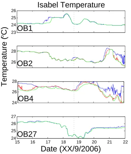
All variables were examined in a 7 day period surrounding the approach and depar-ture of Isabel, 15–22 September 2003. After about the beginning of the day on 20 September, all quantities appeared to have returned to their normal level of variability. 3.1 Temperature (Fig. 2)

5

Waters in OB were warm during Isabel, ranging from 24 to 28◦C. Stratification was very small and temperature differences were minimal for the entire period. (This is not typical for this time of year. Shelf waters are often highly stratified in late summer and early fall.) The exception to that is offshore at OB2 and especially OB4 which show some stratification near the surface. Most typical is the record at OB27. Before Isabel,

10

the temperature was relatively constant at around 26–26.5◦C. As Isabel approached, the temperature dropped about 2◦C to a minimum of 24◦C just after landfall. It then rose again to a constant level of 25.5◦C. Thus, in the period before and after Isabel, the water column decreased in temperature by 0.5◦C. OB1 shows some similar but inverse behavior. During the storm, the temperature actually increased, but then dropped again

15

to a level about 0.1◦C cooler than before the storm. At OB2 and OB4, the picture is more complicated. OB4 showed no particular storm effects on temperature. If the be-ginning of 20 September is chosen as the “after-storm” time, the temperature appears to have increased slightly during the storm. For OB2, the temperature decreased by 2◦C, again if 20 September is the after-storm time.

20

Of course, the temperatures shown in Fig. 2 do not represent a single water mass. Some of the temperature changes seen in Fig. 2 are possibly due to advection of warmer or cooler water. A progressive vector diagram (PVD) was created from the low pass currents for OB27 (not shown). This analysis indicated that waters initially at OB27 were advected 30 km to the southwest during the first part of the storm and then

25

advected back during the latter part. The final position from the PVD on 22 September is within 1 km of the initial position on 15 September. In other words, water advected

(9)

OSD

Full Screen / Esc

EGU away from OB27 during storm and advected back as it departed. Assuming that this

is true, and also assuming the entire water column was completely mixed, we can use the change in temperature and the water depth to get an estimate of the net heat flux. Hurricane Isabel’s winds impacted OB for about 24 h. If we use this time period and the water depths in Table 1, we get a net heat flux of 750 W/m2 at OB27. Although

5

there is no way to verify this number, or provide error bounds, it is certainly a plausible estimate of the heat flux during a storm event like this (Jacob et al., 2000).

To get a larger picture of the temperature field on the shelf, we examined before and after AVHRR SST images (Fig. 3a–c). The before image shows a nearshore plume of cool water moving down the coast around Cape Hatteras just past Cape Lookout.

10

This is a typical feature for this area (Pietrafesa et al., 1994). A cold core Gulf Stream filament is impinging on the continental shelf. Its warm streamer is especially visible at OB2 and OB4. Again this is typical for this area (Pietrafesa et al., 1985a). The after-storm image (Fig. 3b), shows significant cooling of the inner shelf. The warm waters associated with the Gulf Stream in the before-storm image are further from

15

shore. The Gulf Stream filament is not apparent. The image showing the after-before temperature difference (Fig. 3c) indicates that the magnitude of the cooling across the shelf is approximately 1–3◦C. The cooling is mainly confined inshore of OB2 and OB4. Even greater cooling occurred northeast of Cape Lookout under the track of the storm and offshore of the nearshore plume mentioned above. SST values from the satellite

20

images in Fig. 3a and b are very close to those of Fig. 2, confirming the completely unstratified nature of the shelf waters during this period.

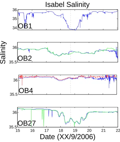
3.2 Salinity (Fig. 4)

Salinity records indicate that salinity was relatively constant and uniform across the mid- and outer shelf prior to the approach of Isabel. Like temperature, there was no

25

salinity stratification during the period of the storm. Late on 17 September, salinity began to drop at all 4 moorings with conductivity sensors. At OB2 and OB4, on the outer shelf, the drop was slight, perhaps 0.1 at the most. At OB27 salinity dropped

(10)

OSD

Full Screen / Esc

EGU about 0.5, to a minimum of about 35.6 late on 18 September. At OB1, salinity reached

a minimum of 33.8 late on 18 September, having dropped almost 2.0 from its pre-storm level. The salinity at OB1 and OB27 then rebounded during 19 September and reached a nearly constant level early on 20 September.

In order to understand these salinity records, we did the following calculation for

5

the record at OB27. We assume, as we did for temperature, that the salinities early on 17 September and early on 20 September represent the same water. That is, water present on 17 September advected away from the site during the storm and then returned approximately by 20 September. During this time, there was storm-related precipitation, which fully mixed in. There was a difference in salinity of about

10

0.1 between 17 September and 20 September. This change in salinity spread out over a 30 m depth represents a net addition of about 8 cm of water at the surface. Note that the salinity change between 17 September and the minimum late on 18 September is about 0.5. If this were the same water this would represent a net precipitation of about 41 cm. This is far too high a value to be plausible given the rainfall measured nearby on

15

land (Bevin and Cobb, 2004). Thus, we have to guess that the large drop in salinity was not entirely a result of net precipitation, but must be due at least in part to advection.

Using the previously quoted heat flux value of 750 W/m2 at OB27 over a period of 24 h (and assuming this is entirely due to latent cooling) gives an evaporation from the surface of about 3 cm. Thus, with a net addition of 8 cm of water to the surface,

20

and 3 cm of evaporation, we calculate 11 cm of rainfall. The National Weather Service Forecast Office in Wilmington, NC reported a total rainfall of 5.03 cm (1.9800) while Bevin and Cobb (2004) reported 4–7 inches (10–18 cm) throughout eastern North Carolina. For 11 cm of rain spread out over 24 h, the rain rate would be calculated as almost 5 mm/hr.

25

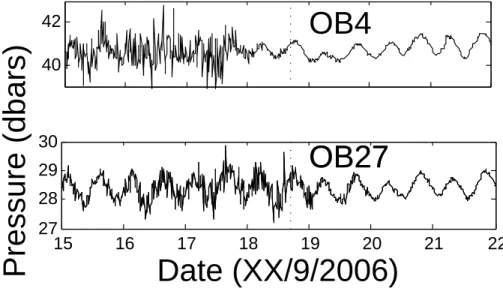
3.3 Pressure and sea level (Figs. 5 and 6)

Bottom pressures at OB4 and OB27 showed no indication of storm surge on the mid-and outer shelf (Fig. 5). The records are somewhat aliased, having been sampled

(11)

OSD

Full Screen / Esc

EGU at 15 and 5 min intervals (Table 1) underneath an energetic field of surface waves.

The surface wave field was apparent as a large increase in high frequency variability as the storm approached. The pressure sensors at OB4 and OB27 were at about 40 and 28 m depth. At this depth, pressure sensors only detect signals from surface waves of periods 8–10 s or greater, i.e. swell. Thus, the high frequency variability is

5

a measure of the energy in the swell. Interestingly, this high frequency variability died down at OB4 around the end of the day on 17 September, almost a day earlier than it did at OB27. As we will see later, the high frequency variability of the pressure at OB27 decreased at about the same time as the swell energy at OB1. The high frequency variability at OB4 also increased much sooner than OB27. It is not clear

10

whether the difference between the pressure records at the two locations is a result of the geographic difference between them, the different depths of the sensors, or local topographic variations that might have focused or diffused the swell arriving from the distant storm.

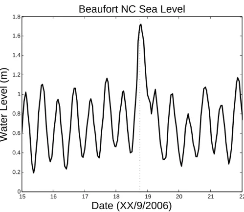
By contrast, sea level at Beaufort Inlet, NC (Fig. 6) showed a storm surge of about

15

70 cm above predicted high tide. The highest sea level at Beaufort was reached at 1900 on 18 September.

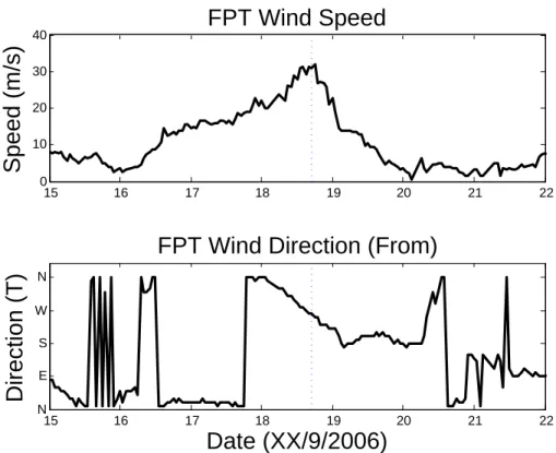
3.4 Winds (Animation 1 and Figs. 7 and 8)

Winds at Frying Pan Tower were light and steady out of the north and northeast before the arrival of Isabel. They began to increase in speed around the middle of 16

Septem-20

ber. Between 12:00 on 16 September and 12:00 on 17 September, the wind increased steadily but the direction did not change much. Around 12:00 on 17 September, the wind direction began to back slowly towards the north. At 00:00 on 18 September, the wind direction began to back rapidly as the storm approached, from north around to northwest and west. At landfall the wind was from the west southwest and

rotat-25

ing rapidly. After landfall, the wind rotated until it was from the south at 03:00 on 19 September, and then diminished quickly. By 00:00 on 20 September, the winds be-came light and variable, showing no further signs of the storm.

(12)

OSD

Full Screen / Esc

EGU Figure 7 has the same data in a different perspective, showing the magnitude and

direction. Here we can see the gradual rise and quick decrease of the wind speed along with the rapid rotation during between 00:00 on 18 September and 03:00 on 19 September. Maximum sustained winds at FPT were 32 m/s at 18:00 on 18 September. Of course the winds at the mooring locations might have been different. However, given

5

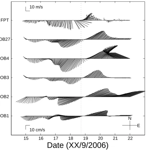
the tremendous size of Isabel, not likely by very much (see e.g. Fig. 1). 3.5 Low pass current (Animation 1 and Figs. 8 and 9)

Before the arrival of Isabel, the currents at all moorings were weak and slowly rotating counterclockwise. They maintained this motion until 06:00 on 16 September. At that time, current vectors at all of the moorings suddenly turned and pointed towards the

10

southwest. By 00:00 on 18 September, currents at all moorings were pointed towards the southwest and increasing in speed. There is an indication throughout that currents were turning along the shelf to follow the cuspate shape of the coastline. For example, the current at OB1 pointed more towards the west than that at OB3. The currents all reached their maximum speed towards the southwest around 09:00 on 18

Septem-15

ber. At that point, the currents began to diminish rapidly. The current speeds at all the moorings reached their minimum at nearly the same time, around 19:00–22:00 on 18 September. The currents then increased rapidly in speed towards the northeast, reaching maximum speed about 12:00 on 19 September. After this point, currents at the inner and mid-shelf moorings diminished rapidly. At the offshore moorings current

20

speeds remained high, but the two moorings seemed to lose their coherence. After the passage of the storm, currents began to behave independently at the different moor-ings, in sharp contrast to the high coherence displayed between 06:00 16 September and 12:00 19 September.

Figure 9 displays the same information in a different way for OB27 only. Here one

25

can see the increase in speed towards the southwest after 06:00 16 September to a maximum of 32 cm/s at 05:45 18 on September. There is a rapid reversal towards the northeast with the speed going to a minimum at 20:30 on 18 September. The maximum

(13)

OSD

Full Screen / Esc

EGU towards the northeast is reached at 11:15 19 September.

With the entire shelf moving as a slab, the low pass flows seemed to be confined to the alongshore direction. In the hours before the flow reversal (17:00 17 September– 09:00 18 September), the currents appeared to rotate a little bit in the same direction as the wind, but are mainly along-shelf. The flow reversal occurs just as the wind rotated

5

enough to where its along-shelf component is upshelf rather than downshelf. That is, the reversal occurred just as the wind vector rotated through a direction more or less perpendicular to the coast. This suggests that the currents were mechanically forced by the wind as it picked up on 16 and 17 September. Ekman dynamics then became important as the steady north wind had blown long enough for the Coriolis force to

10

have an effect. When the wind began to rotate rapidly with the approach of the storm, direct mechanical forcing again dominated, this time pushing the shelf waters towards the northeast.

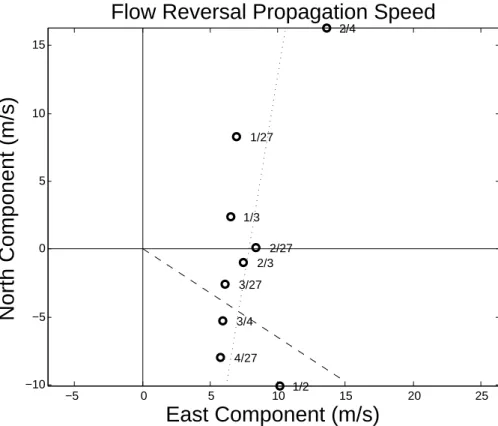
The flow reversal occurred abruptly but not uniformly across the shelf. We used the time at which the speed goes to a minimum (Table 2) as the approximate time

15

of the reversal at each mooring. Generally the reversal proceeded up the coast from southwest to northeast and inshore to offshore. OB3 was first, OB27 second, then OB1 and the two offshore moorings. The greatest difference between times was 03:45 between OB3 and OB2. Each of these time differences implies a propagation speed and direction. This information is presented in Fig. 10. If the reversal were a pure

20

shallow water plane wave propagating in a constant direction at a constant speed, these points would lie on a straight line and the closest approach of the line to the origin would give the magnitude and direction of the propagation vector. For reference, two lines are added to Fig. 9, one is pointed from the origin 33◦ to the south of east. This line is the approximate offshore direction. The other is the least squares fit to the

25

data in the plot. The propagation associated with OB3, the shallowest mooring, was apparently slower than this line would indicate, while the propagation associated with OB2 and OB4, the deeper moorings were faster. This suggests that the propagation sped up as it moved from the inner to the outer shelf, as expected for a shallow water

(14)

OSD

Full Screen / Esc

EGU wave.

Obviously, the flow reversal was not a pure plane wave. The direction and speed could have changed due to refraction from changing bottom depth. The propagation speed is somewhat slower than the local shallow water wave speed, c=√(gH), where g is gravity and H is the depth. If the bottom depth is 15–40 m, this gives wave speeds of

5

12–20 m/s. The direction of propagation is slightly to the south of east. This is close to directly offshore, the dashed line in the figure. Thus the flow reversal propagated in the offshore direction at nearly the speed of a shallow water wave. Keen and Glenn (1999) have shown a hurricane disturbance creating a barotropic Kelvin wave. Here this is unlikely. A Kelvin wave would propagate along the coast, not across the shelf towards

10

deep water. On the other hand, if the flow reversal were a pure shallow water wave, one would expect the water motion associated with it to be in the direction of propagation, not almost perpendicular. Finally, if the flow reversal were a Kelvin wave, one would expect a correlated response in the bottom pressure. Examination of bottom pressure at between OB4 and OB27 (not shown) did not indicate any connection between the

15

observed flow reversal and bottom pressure or bottom pressure gradient. Thus the observed flow reversal was not a Kelvin wave or a shallow water wave. It was some kind of disturbance that propagated offshore but whose flow was confined to the alongshore direction.

With all of the interesting detail in the low pass currents, we make note of the one

20

thing that is missing. There was no apparent response in the inertial or near-inertial band, likely due to the lack of stratification.

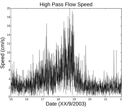
3.6 High pass current (Fig. 11)

The high pass currents at OB27 intensified as the storm approached, reaching a max-imum amplitude of 10–12 cm/s close to the time of landfall and abruptly dying down

25

afterwards. The increase in amplitude of the high frequency variability closely followed the increase in wind speed, the high frequency variability of the bottom pressure and the significant wave height (compare with Figs. 5, 7 and 12). Further analysis of the

(15)

OSD

Full Screen / Esc

EGU high-pass flow (not shown) showed that it was isotropic, and had vertical decorrelation

scales of about 5 m. This high-pass flow was not simply aliased surface waves, be-cause the sampling was specifically designed to remove the effects of surface waves by averaging over a one minute period (Table 1). The flows could conceivably be a result of the way that ADCP data were collected and calculated, with four acoustic

5

beams averaged into each ensemble (Gordon, 1996). However, a similar type of flow has been observed in response to an impulsive wind in current data collected from a non-acoustic current meter (Klinck et al., 1981). Comparison of kinetic energy spectra from the time of the storm’s approach with spectra from a similar length calm period (not shown) indicate a significant elevation of kinetic energy at periods between 10 min

10

and 2 h. The OB27 instrument was not set up to measure flows with periods between 1 and 10 min, so some energy at these periods may not be apparent in this record.

We searched for vertical propagation of signals within this flow by doing time lag correlations between different bins of ADCP data. For example, we could not find significant correlations at any time lag between high frequency flows at 10 m and flow

15

at 20 m. This suggests that these flows were not propagating signals up or down the water column. The lack of stratification makes it unlikely that these flows were the result of internal waves.

3.7 Surface waves (Fig. 12 and Animation 2)

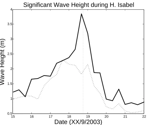
The significant wave height is calculated as four times the square root of the value

20

obtained by integrating the non-directional spectrum from the time series of the surface level (RD Instruments, 2004). Thus, the square of the significant wave height gives an estimate of the total energy in the wave field as a function of time. Significant wave height at OB1 and OB3 show peak heights of close to 4 m at OB1 and 2–2.5 m at OB3. The peak wave heights were reached at OB3 at 17 September at 16:00, and wave

25

heights stayed high for over 24 h. Peak significant wave height at FPT (not shown) was reached at the same time as OB3 and was about 6 m. At OB1, the peak was reached just before Isabel made landfall on 18 September at 16:00. Note the wave

(16)

OSD

Full Screen / Esc

EGU field was sampled only every 4 h, making determination of the peak wave height and

timing inexact. At OB1, the wave heights built up slowly over 3–4 days, until landfall, and then dropped abruptly during the day on 19 September. At OB3, the increase and decrease were more symmetric.

Animation 2 presents directional wave data as a function of time for OB1. (An

an-5

imation from OB3 is omitted for brevity because the results were similar.) Even on 15 September, the energy in the swell was elevated as the storm produced waves far away in the North Atlantic. The swell built up as the storm approached and reached a maximum level around 12:00 on 17 September (bottom left panel). After that, the swell energy decreased. For most of the time there was a clear spectral gap between the

10

swell and wind waves (top left panel).

The wind wave spectrum started out small and did not start building up until about 16:00 on 16 September. At that time the wind waves were coming from the east, while the wind itself was out of the north-northeast. The wind waves continued to build, com-ing mainly from the east, until 04:00 on 18 September. After that, the wind direction

15

began to rotate rapidly. The principal direction of the wind waves followed the rotation of the wind direction, staying 45–90 degrees behind the wind as it rotated. From the directional spectrum on 18 September, it appears the high frequency wind waves ro-tated in direction more quickly than the lower frequency wind waves. Note especially the directional spectrum at 08:00 on 18 September. The wind waves reached a peak

20

at 00:00 on 19 September when the wind wave direction was the same as that of the wind, out of the southwest. At that point, the wind wave field diminished quickly to very low levels. There was very little wave energy in the wind waves or the swell by 00:00 on 20 September. The build-up of wind wave energy followed closely the increase of wind speed at FPT.

25

It is of note here that the wind wave energy and the swell energy peaked 36 hours apart, the wind waves at 00:00 on 19 September and the swell at 12:00 on 17 Septem-ber. The total energy in the wave field peaked somewhere in the middle, near the time of landfall as indicated by the significant wave height. The composition of the wave field

(17)

OSD

Full Screen / Esc

EGU changed dramatically in frequency and direction throughout the duration of the event.

4 Discussion

Hurricane Isabel was a significant low frequency current event in Onslow Bay, but barely rose above the normal fluctuations of the tides. The storm moved quickly, but due to its huge size impacted Onslow Bay for a long period of time. Wind speeds

5

were over 10 m/s for about 3 days (Fig. 7). Speckhart (2004) examined the effects of three hurricanes, Dennis, Floyd and Irene, on Onslow Bay in 1999. Of the three, Dennis had the strongest effect on temperature and dynamics. This was not because it had the strongest winds, but because of the long duration of high winds. Dennis sat nearly motionless for several days offshore of Cape Hatteras while nearly steady

10

10 m/s winds blew over the Bay. Examination of the four year record we have of flows at OB27 indicates that Hurricane Isabel was a particularly energetic event in terms of the larger-scale low frequency response presented in the Animation 1. We speculate that this is a result of the size and duration of the event as opposed to the magnitude of the winds.

15

In the fall, the water column in Onslow Bay normally begins to cool gradually as part of the seasonal cycle. However, that cooling mainly occurs in November and Decem-ber, well after the passage of Isabel. While the 0.5◦C drop in temperature at OB27 (Fig. 2) is associated with the large latent heat flux due to the storm, the size of the change is small compared to fluctuations normally observed at the site.

Tempera-20

ture can change because of seasonal cooling or heating, the passage of fronts, both oceanic and atmospheric, and the upwelling of cool water from the shelf edge. Exam-ination of temperature records leads to the conclusion that while Hurricane Isabel had a large temporary effect, in general such storms are a small part of the heat budget for Onslow Bay. The same conclusion can be made for salinity and the freshwater budget.

25

In terms of the impact on sediments and biota, the most important effect of the storm was in the wave field. Marshall (2004) reported wave orbital velocities of 60–70 cm/s

(18)

OSD

Full Screen / Esc

EGU at OB27 at the height of Isabel. This is far higher than the 20–30 cm/s amplitude of the

tides or the 30 cm/s amplitude of the low frequency response shown in Figs. 7, 8 and Animation 1. As Marshall reported, this made Isabel an extremely unusual event in its ability to mobilize find-grained sediments.

While some aspects of the ocean’s response to Isabel remain mysterious, what is

5

clear from this study is the value of a well-designed and instrumented array to under-standing the impact that such storms can have on the coastal ocean. As more such arrays are built under the auspices of the Integrated Ocean Observing System (IOOS), we will have many more opportunities to study how storms like Isabel change the ocean environment that they pass over.

10

Acknowledgements. Mooring data were collected under the auspices of CORMP, which is

funded by NOAA. Technical support with data collection was provided by J. Souza, D. Wells, B. Sweet, J. Kinder, and others. The code for displaying the waves data was generously pro-vided by G. Voulgaris. Model wind data in Fig. 1 and storm track data in Animation 1 were downloaded from NOAA’s Hurricane Research Division. AVHRR data in Fig. 3 were provided 15

by Rutgers University’s Coastal Ocean Observation Lab, with special help from J. Bosch. I had helpful comments from M. Durako, G. Snedden and J. Morrison.

References

Bevin, J. and Cobb, H.: Tropical Cyclone Report, Hurricane Isabel, 6–19 September 2003, National Hurricane Center, Miami Fl, 2004.

20

Chu, P. C., Veneziano, J. M., Fan, C., Carron, M. J., and Liu, W. T.: Response of the South China Sea to Tropical Cyclone Ernie 1996, J. Geophys. Res., 105(C6), 13 991–14 009, 2000. Geisler, J. E.: Linear Theory of the Response of a Two Layer Ocean to a Moving Hurricane,

Geophys. Fluid Dyn., 1, 249–272, 1970.

Ginis, I. and Sutyrin, G. G.: Hurricane-generated Depth-averaged Currents and Sea Surface 25

Elevation, J. Phys. Oceanogr., 25, 1218–1242, 1995.

Gordon, R. L.: Acoustic Doppler Current Profiler Principles of Operation A Practical Primer, 1–54 pp., RD Instruments Inc., San Diego, 1996.

(19)

OSD

Full Screen / Esc

EGU

Jacob, S. D., Shay, L. K., Mariano, A. J., and Black, P. G.: The 3D Oceanic Mixed Layer Response to Hurricane Gilbert, J. Phys. Oceanogr., 30(6), 1407–1429, 2000.

Keen, T. R. and Glenn, S. M.: Shallow water currents during Hurricane Andrew, J. Geophys. Res., 104(C10), 23 443–23 458, 1999.

Klinck, J. M., Pietrafesa, L. J., and Janowitx, G. S.: Continental Shelf Circulation Induced by a 5

Moving, Localized Wind Stress, J.Phys.Oceanogr., 11(6), 836–848, 1981.

Marshall, J. A.: Event Driven Sediment Mobility on the Inner Continental Shelf of Onslow Bay, NC, Masters Thesis, University of North Carolina Wilmington, 1–90, 2004.

Murray, S. P.: Bottom Currents Near the Coast during Hurricane Camille, J. Geophys. Res., 75(24), 4579–4582, 1970.

10

Pietrafesa, L., Janowitz, G. S., and Wittman, P. A.: Physical Oceanographic Processes in the Carolina Capes, in: Oceanography of the Southeastern U.S. Continental Shelf, edited by: Atkinson, L. P., Menzel, D. W., and Bush, K. A., pp. 23–32, American Geophysical Union, Washington DC, 1985a.

Pietrafesa, L. J., Blanton, J. O., Wang, J. D., Kourafalou, V., Lee, T. N., and Bush, K. A.: The 15

Tidal Regime in the South Atlantic Bight, in: Oceanography of the Southeastern U.S. Conti-nental Shelf, edited by: Atkinson, L. P., Menzel, D. W., and Bush, K. A., pp. 63–76, American Geophysical Union, Washington DC, 1985.

Pietrafesa, L. J., Morrison, J. M., McCann, M. P., Churchill, J., Boehm, E., and Houghton, R. W.: Water mass linkages between the Middle and South Atlantic Bights, Deep-Sea Res. II, 20

41, 365–389, 1994.

Price, J. F.: Internal Wave Wake of a Moving Storm. Part I: Scales, Energy Budget and Obser-vations, J. Phys. Oceanogr., 13, 949–965, 1983.

Price, J. F.: Upper Ocean Response to a Hurricane, J.Phys.Oceanogr., 11, 153–175, 1981. Price, J. F., Sanford, T. B., and Forristall, G. Z.: Forced Stage Response to a Moving Hurricane, 25

J. Phys. Oceanogr., 24, 233–260, 1994.

RD Instruments Inc.: WAVES PRIMER: Wave Measurements and the RDI ADCP Waves Array Technique, 1–22 pp., RD Instruments Inc., San Diego CA, 2004.

Shay, L. K. and Chang, S. W.: Free Surface Effects on the Near-inertial Current Response to A Hurricane: A Revisit, J. Phys. Oceanogr., 27, 23–39, 1997.

30

Shay, L. K. and Elsberry, R. L.: Near-inertial ocean current response to Hurricane Frederic, J. Phys. Oceanogr., 17(8), 1249–1269, 1987.

(20)

OSD

Full Screen / Esc

EGU

to a Hurricane, J. Phys. Oceanogr., 19, 649–669, 1989.

Smith, N. P.: Longshore Currents on the Fringe of Hurricane Anita, J. Geophys. Res., 83(C12), 6047–6051, 1978.

Smith, N. P.: Response of Florida Atlantic Shelf Waters to Hurricane David, J. Geophys. Res, 87(C3), 2007–2016, 1982.

5

Speckhart, B. L.: Observational analysis of shallow water response to passing hurricanes in Onslow Bay, NC in 1999, Masters Thesis, University of North Carolina Wilmington, 1–61, 2004.

Walsh, E. J., Wright, C. W., Vandemark, D., Krabill, W. B., Garcia, A. W., Houston, S. H., Murillo, S. T., Powell, M. D., Black, P. G., and Marks Jr., F. D.: Hurricane Directional Wave Spectrum 10

Spatial Variation at Landfall, J. Phys. Oceanogr., 32(6), 1667–1684, 2002.

Williams, W. J., Beardsley, R. C., Irish, J. D., Smith, P. C., and Limeburner, R.: The response of Georges Bank to the passage of Hurricane Edouard, Deep-Sea Res. II Top. Stud. Oceanogr., 48(1–3), 179–197, 2001.

Withee, G. W. and Johnson, A.: Data Report: Buoy Observations during Hurricane Eloise 15

(September 19 to October 11, 1975), 21 pp., Washington, DC, 1988.

Wren, P. A. and Leonard, L. A.: Sediment transport on the mid-continental shelf in Onslow Bay, North Carolina during Hurricane Isabel, Estuar. Coast. Shelf Sci., 63(1–2), 43–56, 2005. Xie, L., Pietrafesa, L. J., Bohm, E., Zhang, C., and Li, X.: Evidence and mechanism of Hurricane

Fran-induced ocean cooling in the Charleston Trough, Geophys. Res. Lett., 25(6), 769–772, 20

(21)

OSD

Full Screen / Esc

EGU

Table 1. Configuration of CORMP Instrumentation.

Site Name OB1 OB2 OB3 OB4 OB27 Location 34 18.639N 33 59.091N 34 06.133N 33 35.398N 33 58.858N

77 03.010W 76 39.211W 77 45.049W 77 03.053W 77 21.738W Bottom Depth (m) 25 40 16 40 30

ADCP Situation On bottom looking upward 2 m above bottom looking upward Frequency 300 kHz 300 kHz 1200 kHz 300 kHz 600 kHz Sampling details 1 h ensembles, 80 pings per ensemble, pings evenly spaced in time 5 min ensembles,

30 pings per ensemble over a one minute period Nominal depth of 10 m 20 m 8 m 20 m 10 m

data used in this study

Waves 4 h sampling Yes, but not 4 h sampling No No Measurements described here

Conductivity, Situation 15 m and 15 m, 30 m* none 15 m, 30 m 12 m and Temperature bottom* and bottom and bottom* 27 m Logger

Sampling Interval 15 min 5 min Bottom None 15 min 5 min Pressure sampling sampling Sensor

* Conductivity/salinity data not discussed or shown for these instruments due to data quality problems.

(22)

OSD

Full Screen / Esc

EGU

Table 2. Time on 18 September when the flow speed becomes a minimum at each mooring.

OB1 OB2 OB3 OB4 OB27

(23)

OSD

Full Screen / Esc

EGU

Fig. 1. Wind speed at 16:30 on 18 September 2003. Color bar at right gives scale in m/s.

Winds obtained from the Hurricane Research Division. Note the eye of the storm passing over Drum Inlet, NC. Also shown are the locations of the 5 CORMP moorings, OB1, OB2, OB3, OB4 and OB27 (Table 1), and Frying Pan Tower (FPT). At each mooring location and at FPT, wind vectors are displayed showing the modeled direction and speed, with winds generally blowing towards the east or southeast. A scale for the wind vectors is shown at the upper left along with an inset map showing the location of the study area relative to the southeastern United States. Cape Fear and Cape Lookout are shown. Onslow Bay is the area between these capes. The “B” near Cape Lookout is the location of Beaufort Inlet.

(24)

OSD

Full Screen / Esc

Printer-friendly Version Interactive Discussion EGU 23 24 25 26

Isabel Temperature

OB1

26 28

Temperature (

°

C)

OB2

24 26 28

OB4

15 16 17 18 19 20 21 22 24 25 26 27

Date (XX/9/2006)

OB27

Fig. 2. Temperature at 4 moorings during the period surrounding the landfall of Hurricane

Is-abel. Green curves are lower or bottom instruments. Blue curves are upper or 15 m instruments

and red curves are lower or 30 m instruments (see Table 1). Note different temperature scales

(25)

OSD

Full Screen / Esc

EGU

(a) (b)

(c)

Fig. 3. (a) AVHRR MCSST Temperature (◦C) image from 15 September 2003 at 22:00. Color-bar at right indicates temperature scale. Locations of CORMP moorings and FPT are shown

on map (see Fig. 1). (b) Same as (a) but for 19 September 2003 at 22:54. (c) Temperature

(26)

OSD

Full Screen / Esc

Printer-friendly Version Interactive Discussion EGU 34 35 36

Isabel Salinity

OB1

35.5 36

Salinity

OB2

35.5 36

OB4

15 16 17 18 19 20 21 22 35.5 36

Date (XX/9/2006)

OB27

Fig. 4. As in Fig. 2, but for salinity. Note some records are not plotted because data were not

(27)

OSD

Full Screen / Esc

Printer-friendly Version Interactive Discussion EGU 40 42

Pressure (dbars)

OB4

15 16 17 18 19 20 21 22 27 28 29 30

Date (XX/9/2006)

OB27

(28)

OSD

Full Screen / Esc

Printer-friendly Version Interactive Discussion EGU 15 16 17 18 19 20 21 22 0 0.2 0.4 0.6 0.8 1 1.2 1.4 1.6 1.8

Date (XX/9/2006)

Water Level (m)

Beaufort NC Sea Level

(29)

OSD

Full Screen / Esc

Printer-friendly Version Interactive Discussion EGU 15 16 17 18 19 20 21 22 0 10 20 30 40

FPT Wind Speed

Speed (m/s)

15 16 17 18 19 20 21 22 N E S W N

FPT Wind Direction (From)

Direction (T)

Date (XX/9/2006)

(30)

OSD

Full Screen / Esc

Printer-friendly Version Interactive Discussion EGU 15 16 17 18 19 20 21 22 OB1 OB2 OB3 OB4 OB27 FPT

Date (XX/9/2006)

10 cm/s 10 m/s N E

Fig. 8. Stick diagram of winds at FPT (top series) and low-pass currents at other moorings as

(31)

OSD

Full Screen / Esc

Printer-friendly Version Interactive Discussion EGU 15 16 17 18 19 20 21 22 0 10 20 30

40

OB27 Current Speed

Speed (cm/s)

15 16 17 18 19 20 21 22 N E S W

N

OB27 Current Direction (To)

Direction (T)

Date (XX/9/2006)

(32)

OSD

Full Screen / Esc

Printer-friendly Version Interactive Discussion EGU −5 0 5 10 15 20 25 −10 −5 0 5 10 15 1/2 1/3 1/27 2/3 2/4 2/27 3/4 3/27 4/27

Flow Reversal Propagation Speed

East Component (m/s)

North Component (m/s)

Fig. 10. Propagation of the flow reversal across the CORMP array. Individual points are labeled

with the appropriate pair of moorings. For example, point labeled “1/27” shows the speed and direction of propagation of the flow reversal from OB1 to OB27. Dotted line is a least squares

fit to the points shown. Dashed line points 33◦ below the x-axis, approximately the offshore

(33)

OSD

Full Screen / Esc

Printer-friendly Version Interactive Discussion EGU 15 16 17 18 19 20 21 22 0 2 4 6 8 10 12 14 16 18

20

High Pass Flow Speed

Speed (cm/s)

Date (XX/9/2003)

Fig. 11. Speed of the high pass flow at OB27.

(34)

OSD

Full Screen / Esc

Printer-friendly Version Interactive Discussion EGU 15 16 17 18 19 20 21 22 0.5 1 1.5 2 2.5 3 3.5 4

Wave Height (m)

Date (XX/9/2003)

Significant Wave Height during H. Isabel

Fig. 12. Significant wave height (m) at OB1 (solid) and OB3 (dashed). Small dotted lines show

(35)

OSD

Full Screen / Esc

EGU

Animation 1 (http://www.ocean-sci-discuss.net/3/1681/2006/osd-3-1681-2006-supplement.

zip). Hourly wind and low pass currents in Onslow Bay, NC. Black circles represent

moor-ing locations OB1-4 and 27 (see Fig. 1). Low pass currents are displayed as blue vectors with tails at mooring locations. The green dot is Frying Pan Tower, with hourly wind displayed as a green vector. Scale bars are shown in upper left, blue for current and green for wind. Hurricane track is shown as blue circles. Double blue circles are positions of the eye of Hurricane Isabel obtained from the Hurricane Research Division. Single blue circles are interpolated positions at times between the given positions at the double blue circles. The time and date of each frame are shown at the lower left. Towards the end of the animation, the hurricane eye can be seen moving through the frame to the northwest as a series of red circles that progressively cover the blue track as the eye passes.

(36)

OSD

Full Screen / Esc

EGU

Animation 2 (http://www.ocean-sci-discuss.net/3/1681/2006/osd-3-1681-2006-supplement.

zip). Directional wave spectral information from OB1. Time and date are indicated at the top

left. Upper left panel. Wave spectra integrated over direction as a function of frequency. The

boundary between the red and blue parts of the curve at f=1/8 s is taken to be the boundary

between the wind waves (red) and the swell (blue), Lower left panel. Wave spectra integrated over frequency as a function of direction. Direction for waves is where they come from. Blue is the swell and red is the wind waves as defined in the upper left panel. The black line is the wind (from) direction. The position of the black dot that moves up and down on this line is proportional to the wind speed. Right panel. Full directional spectrum, with color bar at bottom.