Trends and variability in stratospheric mixing: 1979?2005

(1)

HAL Id: hal-00302752

https://hal.archives-ouvertes.fr/hal-00302752

Submitted on 10 May 2007

HAL is a multi-disciplinary open access

archive for the deposit and dissemination of sci-entific research documents, whether they are pub-lished or not. The documents may come from teaching and research institutions in France or abroad, or from public or private research centers.

L’archive ouverte pluridisciplinaire HAL, est destinée au dépôt et à la diffusion de documents scientifiques de niveau recherche, publiés ou non, émanant des établissements d’enseignement et de recherche français ou étrangers, des laboratoires publics ou privés.

Trends and variability in stratospheric mixing:

1979?2005

H. Garny, G. E. Bodeker, M. Dameris

To cite this version:

H. Garny, G. E. Bodeker, M. Dameris. Trends and variability in stratospheric mixing: 1979?2005. Atmospheric Chemistry and Physics Discussions, European Geosciences Union, 2007, 7 (3), pp.6189-6228. �hal-00302752�

(2)

ACPD

7, 6189–6228, 2007

Trends and variability in stratospheric mixing H. Garny et al. Title Page Abstract Introduction Conclusions References Tables Figures ◭ ◮ ◭ ◮ Back Close

Full Screen / Esc

Printer-friendly Version Interactive Discussion

EGU

Atmos. Chem. Phys. Discuss., 7, 6189–6228, 2007 www.atmos-chem-phys-discuss.net/7/6189/2007/ © Author(s) 2007. This work is licensed

under a Creative Commons License.

Atmospheric Chemistry and Physics Discussions

Trends and variability in stratospheric

mixing: 1979–2005

H. Garny1, G. E. Bodeker2, and M. Dameris3 1

Meteorological Institute, University of Munich, Munich, Germany 2

National Institute of Water and Atmospheric Research, Lauder, New Zealand 3

DLR-Institut f ¨ur Physik der Atmosph ¨are, Oberpfaffenhofen, Germany Received: 5 April 2007 – Accepted: 21 April 2007 – Published: 10 May 2007 Correspondence to: G. Bodeker (g.bodeker@niwa.co.nz)

(3)

ACPD

7, 6189–6228, 2007

Full Screen / Esc

Abstract

Changes in climate are likely to drive changes in stratospheric mixing with associated implications for changes in transport of ozone from tropical source regions to higher latitudes, transport of water vapour and source gas degradation products from the tropical tropopause layer into the mid-latitude lower stratosphere, and changes in the

5

meridional distribution of long-lived trace gases. To diagnose long-term changes in stratospheric mixing, global monthly fields of Lyapunov exponents were calculated on the 450 K, 550 K, and 650 K isentropic surfaces by applying a trajectory model to wind fields from NCEP/NCAR reanalyses over the period 1979 to 2005. Potential underlying geophysical drivers of trends and variability in these mixing fields were investigated by

10

applying a least squares regression model, which included basis functions for a mean annual cycle, seasonally dependent linear trends, the quasi-biennial oscillation (QBO), the solar cycle, and the El Ni ˜no Southern Oscillation (ENSO), to zonal mean time series of the Lyapunov exponents.

Long-term positive trends in mixing are apparent over southern middle to high

lat-15

itudes at 450 K through most of the year, while negative trends over southern high latitudes are apparent at 650 K from May to August. Wintertime negative trends in mix-ing over northern mid-latitudes are apparent at 550 K and 650 K. Over low latitudes, within 40◦of the equator, the QBO exerts a strong influence on mixing at all three anal-ysis levels. This QBO influence is strongly modulated by the annual cycle and shows

20

a phase shift across the subtropical mixing barrier. Solar cycle and ENSO influences on mixing are generally not significant. The diagnosed long-term changes in mixing should aid the interpretation of trends in stratospheric trace gases.

1 Introduction

Stratospheric mixing, and in particular meridional barriers to stratospheric mixing, play

25

(4)

ACPD

7, 6189–6228, 2007

Full Screen / Esc

EGU

surfaces (Plumb and Ko, 1992). For example, changes in total column ozone in the northern hemisphere have been shown to be linked to interannual variability in lower stratospheric planetary wave breaking (Randel et al.,2002;Hood et al.,1999).

A number of different diagnostics of stratospheric mixing have been developed. The morphology of mixing on isentropic surfaces can be diagnosed from maps of potential

5

vorticity (PV) since PV is a conservative quantity for adiabatic transport and therefore PV contours approximate material contours for time scales where diabatic effects can be neglected. The approach has been used to reveal barriers to meridional mixing as steep gradients in PV fields, and to reveal the presence of filaments of high latitude air in mid-latitudes as tongues of high PV (McIntyre and Palmer,1984;Hoskins et al.,

10

1985). A technique based on advection of material contours has been used to diagnose fine-scale features in mixing and shows very good agreement with observed tracer dis-tributions (Waugh,1993;Waugh et al.,1994). A more recently developed quantity is the effective diffusivity, a modified Lagrangian mean diagnostic, which is derived by trans-forming the tracer transport advection-diffusion equation into a diffusion-only equation

15

by introducing coordinates based on isolines of tracer mixing ratio (Nakamura,1996;

Allen and Nakamura,2001;Haynes and Shuckburgh,2000). Effective diffusivity is then a measure of the geometric complexity of tracer contours. The analyzed tracer field can be based on observations (e.g.Nakamura and Ma,1997) or on an artificial “test tracer” that is advected by analyzed winds (e.g.Shuckburgh et al.,2001;Haynes and

Shuck-20

burgh,2000). Another approach to measure mixing is the use of Lyapunov exponents which measure the separation of two trajectories with time from initially nearby start-ing points. The exponents are related to the local stretchstart-ing deformation of the fluid following an air parcel and have been used to identify mixing and barriers to mixing in the atmosphere (Pierrehumbert and Yang, 1993;Bowman,1993). The concept of

25

Lyapunov exponents was recently used for a new technique to model mixing in a La-grangian model (McKenna et al.,2002). This is the method used to diagnose mixing in the study reported on here.

Using the diagnostics discussed above, stratospheric mixing has been investigated 6191

(5)

ACPD

7, 6189–6228, 2007

Full Screen / Esc

intensively and studies reveal inhomogeneities in mixing determined by regions of strong mixing and barriers to air exchange. Strong barriers to mixing have been identi-fied at the polar vortex edge (McIntyre and Palmer,1984;Bowman,1993). The Antarc-tic vortex shows a more persistent barrier compared to its ArcAntarc-tic counterpart (Allen and

Nakamura,2001;Haynes and Shuckburgh,2000). In the winter mid-latitudes, mixing

5

is generally found to be strong. McIntyre and Palmer (1984), who coined the term “surf-zone” for this region, suggested that breaking of planetary-scale Rossby-waves, that can penetrate vertically from the troposphere into the stratosphere when winds are westerly (and therefore primarily in winter), are the cause of high winter-time mix-ing. Breaking of planetary waves is characterized by rapid and irreversible deformation

10

of material contours. The contours form tongues that become longer and thinner with time, more and more fine-scaled, until the material is diffused into its surroundings (Tan

et al.,1998). The “surf-zone” is bounded on its equatorward edge by a barrier to mixing with tropical air. In the absence of episodic mixing events (Waugh, 1993), this bar-rier separates tropical air from air at higher latitudes and creates a “tropical reservoir”

15

for tracers that are transported into the stratosphere through the tropical tropopause (Trepte and Hitchmann, 1992). The summer hemisphere is generally characterized by weak mixing, since easterly winds prohibit vertical propagation of planetary waves. Changes in this spatial pattern of mixing have been studied previously. For exam-ple,Shuckburgh et al.(2001) investigated the influence of the quasi-biennial oscillation

20

(QBO) on inter-annual changes in tropical mixing over a period of six years.

The goal of this paper is to quantify long-term (1979–2005) trends and variability in stratospheric mixing by applying a regression model to diagnostics of mixing. Potential explanatory factors of the variability, such as the QBO and solar cycle, are investigated by including indices for these factors as basis functions in the regression model. The

25

calculation of the Lyapunov exponents used to diagnose mixing in this study is de-scribed in Sect.2. The regression model used to quantify the trends and variability in the calculated global monthly Lyapunov exponents is described in Sect.3. Examples of hemispheric distributions and zonal means of the calculated Lyapunov exponents

(6)

ACPD

7, 6189–6228, 2007

Full Screen / Esc

EGU

are presented in Sect.4while the results from the application of the regression model are presented in Sect.5. A discussion of these results, and the conclusions drawn, are presented in Sect.6.

2 Lyapunov exponents

In an n-dimensional system, the spectrum of Lyapunov exponents is defined as:

λ_i = lim t→∞ δxi(t0)→0 1 t − t0 ln δxi(t) δx_i(t0) (i = 1...n)

where the λi are the n Lyapunov exponents with initial orientation i of the distance

5

vector between the starting points of two nearby trajectories. Thesen distance

vec-tors are orthogonal with lengthδxi(t0). Theδxi(t) are the distances between the two

trajectories at timet (Bowman,1993;Wolf et al.,1985).

For the purposes of this study, two dimensional (latitude and longitude) Lagrangian forward trajectories are computed on isentropic surfaces using a standard 4th order

10

Runge-Kutta integration scheme (Press et al.,1989) applied at 1 hour integration in-tervals to 6 hourly 2.5◦×2.5◦ NCEP/NCAR wind fields on the 450, 550 and 650 K isen-tropes. The zonal and meridional wind components are interpolated to the location of the advected air parcels using bilinear spatial interpolation and linear interpolation in time. Trajectories within 20◦ of the poles are transformed to a Cartesian coordinate

15

system to avoid the singularity at the pole which occurs when prescribing winds using zonal and meridional components. In this two dimensional system, two Lyapunov ex-ponents, with initially perpendicular distance vectors, can be defined. As discussed in

Pierrehumbert and Yang (1993), it is sufficient to consider only one of the two expo-nents, since, in making the assumption of incompressible flow, the conservation of the

20

area spanned by the two distance vectors (initially a circle, deformed to an ellipse) is accounted for and therefore no additional information is given by the second Lyapunov exponent.

(7)

ACPD

7, 6189–6228, 2007

Full Screen / Esc

To maintain the condition of small distances between the trajectories (δx_i(t0) → 0), the distance δxi(t), which grows as time proceeds, needs to be periodically

renor-malized. Practically this is done by periodically resetting the distance between the trajectoriesδx_i(t) to δx_i(t0) (Wolf et al.,1985). The Lyapunov exponent for finite time periods, also called the finite time Lyapunov Exponent (FTLE), with renormalization after a periodT is then given by:

λ =_nT1 n X k=1 lnδx(kT ) δx(0)

whereδx(kT ) is the distance after k time intervals of length T , n the total number of

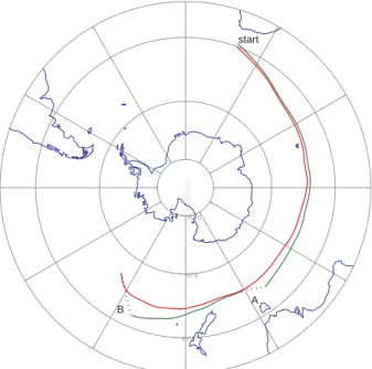
intervals andδx(0) the initial distance at t0=0. Figure1shows two example 12 day tra-jectories on the 450 K level, commencing on 1 August 2000, and where renormalization is applied after 6 days. Distances labelled A and B denoteδx(kT ) (for k=1,2).

McKenna et al.(2002), who use the FTLE as a tool to model mixing in a chemical

5

Lagrangian model, show that FTLEs are directly related to shear and strain rates of the flow. The relation between Lyapunov exponents and mixing, that can be parameter-ized as diffusivity, can be established in the following way (as shown byMcKenna et al.,

2002): since in the calculation of FTLE only diffusion and not advection is accounted for, the corresponding equation for tracer concentrations is a diffusion-only equation,

10

with a solution of the form exp(−₄x_Dt2 ) where _{D is the diffusivity. By assuming that the} distanceδx(T ) represents the halfwidth of the tracer distribution after time step T , the

diffusivity can be approximated by δx(T )₄_T 2. By replacingδx(T ) with δx(0) exp λT the

dif-fusivity can then be related to the FTLE (D= const × exp(λ)), and a link between the

physical process of mixing and Lyapunov exponents is established (even though this

15

connection is rather conceptual). Effective diffusivity, a different measure to the diffu-sivity described above, has been used byHaynes and Shuckburgh(2000) to diagnose both stratospheric transport and mixing. While effective diffusivity broadly matches the spatial structure obtained with FTLE (which measures only mixing), disagreements in the small scale structure exist (Shuckburgh and Haynes,2003).

(8)

ACPD

7, 6189–6228, 2007

Full Screen / Esc

EGU

In this study, Lyapunov exponents, with units of day−1, were calculated from 30 day trajectories with a renormalization period of 10 days. Over this period, diabatic ascent and descent rates were assumed to be negligible (Bowman, 1993). The choice of the renormalization period is not critical (Wolf et al., 1985), and calculations of the Lyapunov exponents for varyingT were found to give similar results. The initial distance

5

δx(0) was chosen to be 1 km. The trajectory length of 30 days provides Lyapunov

exponents for each month. However, these are not monthly means but rather should be interpreted as the degree to which an air parcel is deformed, and therefore mixed with surrounding air, over the course of the month. The location identified with a particular Lyapunov exponent is the origin of the calculated trajectories. The resultant monthly

10

Lyapunov exponents are presented in Sect.4.

To investigate the effects of uncertainties in the NCEP/NCAR reanalyses wind fields on the calculated Lyapunov exponents, the calculations were repeated for one year (1984) with wind fields perturbed as follows: Gaussian distributed errors were added to the winds at each grid point, choosing a standard deviation for the u component

15

of 2.5 m s−1 and for the v wind component of 1.5 m s−1 based on the uncertainties reported inKalnay et al.(1996). The resulting relative errors in the Lyapunov exponents are approximately normally distributed with a mean value near zero (−0.0283) and a standard deviation of ∼0.12. These results indicate a sufficient robustness against errors in the wind fields. The time-latitude pattern of zonal mean Lyapunov exponents

20

of the runs with and without errors are well correlated (with a correlation coefficient of ∼0.72).

3 The regression model

To quantify the underlying geophysical drivers of trends and variability in the calculated Lyapunov exponents, zonal means were calculated and analyzed using a least squares

(9)

ACPD

7, 6189–6228, 2007

Full Screen / Esc

regression model of the form

λ_m(φ, t) =a1(φ, t)+ a2(φ, t) · Linear(t)+ a3(φ, t) · QBO(t + ∆t)+ a4(φ, t) · Solar(t)+ a5(φ, t) · ENSO(t) (1)

whereφ is the latitude, t is the time in months (t=1 for January 1979), and λm(φ, t)

is the modelled Lyapunov exponent. The regression model residuals (r(φ, t)) are the

differences between the modelled and calculated Lyapunov exponents. In addition to an offset and mean annual cycle, a linear term, the QBO, the solar cycle, and El Ni ˜no southern oscillation (ENSO) have been included as basis functions. Their coefficients

ai are expanded to account for seasonal variability as follows:

a_i(φ, t) = ai 0(φ) + N X k=1 [a_{i ks}(φ) sin(2πk(t − 0.5)/12)+ +ai kc(φ) cos(2πk(t − 0.5)/12)] (2)

N is set to 4 for the constant terma1, and for all other basis functions it is set to 2, so that the total number of coefficients is 29. This allows variability at annual and semi-annual periods for the coefficients 2 to 5. The coefficients are calculated by minimizing the sum of the squared residuals for each latitude separately. Uncertainties in the regression coefficients were calculated using:

σ_a2_k = χ 2

N − M[(X

T_{X )}−1

]_kk (3)

whereχ2 is the sum of the squared residuals, N is the length of the time series, M

(10)

ACPD

7, 6189–6228, 2007

Full Screen / Esc

EGU

Zwiers, 2002). This method of calculating the uncertainties in the regression coef-ficients assumes that the residuals are white noise i.e. normally distributed with zero mean and statistically independent in time. If this assumption is violated, the uncertain-ties on the model coefficients will be significantly underestimated (Tiao et al.,1990). In these circumstances a more accurate estimate of the uncertainties in the parameters must be calculated by correcting the residual term for its autocorrelation. The method described in Appendix A ofTiao et al.(1990) is applied here. The first step is to run the regression model and obtain the coefficients a1toa5. These coefficients, together with the basis functions, are then used to construct the modelled Lyapunov exponents which are then subtracted from the observed values to derive the residuals. A first order autocorrelation coefficient (̺) is derived by regressing the residuals at time step

t against the residuals at time t − 1. This coefficient is then used to transform the time

seriesλ(φ, t), and the basis functions, as follows: x(t) → x(t) − ̺ · x(t − 1)

The regression model is now rerun with the transformed variables. The corrected vari-ance in the coefficients is obtained as described above (see Eq.3) with the transformed model. The uncertainty estimates when taking autocorrelation into account were al-most twice as high as when neglecting it, which shows the necessity for doing so in this case. The total variance for coefficient ai is obtained by

σ2(ai) =σ2(ai 0) + N X k=1 [σ2(ai ks) sin2(2πk(t − 0.5)/12)]+ + σ2(aikc) cos2(2πk(t − 0.5)/12)]

In the following, coefficients are considered as significant when ai≥2σ(ai), which

cor-responds to a significance level of about 95% (the ratioa_i/σ(a_i) is student-t distributed and converges to the normal distribution forN−M≥30). This means that with a

cer-tainty of 95% the null hypothesisai=0 can be rejected if ai/σ(ai)> 2.

(11)

ACPD

7, 6189–6228, 2007

Full Screen / Esc

The portion of variability in Lyapunov exponents that is explained by the fitted model can be estimated by the coefficient of multiple determination R2 (von Storch and Zwiers,2002), which is given by

R2(_{φ) =} PN i=1(λm(φ, i) − λ(φ))2 χ2₊PN i =1(λm(φ, i) − λ(φ))2 (4)

whereλ(φ) is the mean observed Lyapunov exponent at latitude φ.

The basis functions used for this regression model are indicators of processes that are believed to play a role in the variability in mixing. The first term on the right hand side of Eq. (1) simply represents the mean annual cycle and offset. By choosing N=4 in Eq. (2) periodicities of 12, 6, 4 and 3 months are allowed. The second term represents

5

a linear trend in mixing, and withN=2, allows for trends to be different during different

months of the year with annual and semi-annual structure.

The QBO dominates equatorial dynamics and is highly likely to influence mixing (Shuckburgh et al.,2001). Monthly mean equatorial zonal mean winds at 50 hPa from the NCEP/NCAR reanalyses were used as the QBO basis function, where a time lag

10

∆t was allowed. The optimal value for ∆t was identified by taking the best fit (minimal sum of squared residuals) of runs with ∆t varying from –12 to +12 months.

The 11-year solar cycle shows significant correlations with dynamical quantities such as geopotential height and temperature in the lower stratosphere (van Loon and

Lab-itzke,2000). A solar cycle influence on mixing is therefore conceivable and has been

15

incorporated in the regression model as 10.7 cm solar fluxes measured at Ottawa. ENSO is represented by the southern oscillation index (SOI), the difference in monthly mean sea level pressure between Tahiti and Darwin.

(12)

ACPD

7, 6189–6228, 2007

Full Screen / Esc

EGU 4 Results from lyapunov exponent calculations

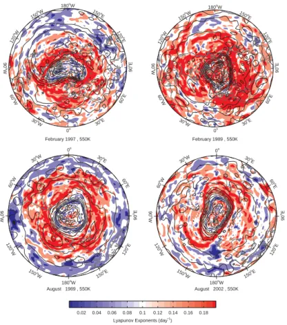
Lyapunov exponents were calculated on a latitude-longitude grid of 180×180 points to provide global coverage at 1◦ latitude and 2◦ longitude resolution. Examples of hemispheric distributions of the calculated Lyapunov exponents are shown in Fig.2.

Because the Lyapunov exponents shown in Fig.2integrate the effects of mixing over

5

a one month period, features with a shorter time-scale, such as tongues of PV in mid-latitudes apparent in the instantaneous PV fields at the start date of the trajectories, would not be reflected in the Lyapunov exponent distributions. However, where features in the PV field persist over time scales on the order of 1 month, the extent of mixing associated with those features is reflected in the Lyapunov exponent distributions.

10

In 1996/1997 the Arctic vortex was weak early in the season and grew rapidly in strength from early 1997 onwards (see further discussion below). In contrast, in 1988/1989 the vortex was strong early in the winter season but was significantly dis-turbed by a sudden stratospheric warming in February 1989. While steep gradients are still visible in the PV field at the start of February, the Lyapunov exponents show

15

strong mixing of air from the interior of the vortex to mid-latitudes. In 1989, the Antarc-tic vortex was strong and well formed by August. In 2002 the early August vortex is very elongated and the Lyapunov exponents suggest that there was mixing across the vortex edge (the region of steep gradients in PV).

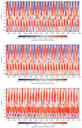
For the analyses presented below, the Lyapunov exponents were zonally averaged,

20

based on their starting coordinates, and are shown in Fig.3 for 1979 to 2005. Note the different colour scaling in the three panels, resulting from increasing variability in mixing with height. A clear annual cycle can be seen at all levels, and in the latitudes mixing is generally high in winter and low in summer. Over southern mid-latitudes at 450 K, the annual cycle is very weak. At 550 K and 650 K, the region of high

25

mixing in winter mid-latitudes, the stratospheric “surf zone”, is equally strong in both hemispheres but extends over a greater range of latitudes in the northern hemisphere. At these two levels, mixing is weaker in summer in the northern hemisphere than in the

(13)

ACPD

7, 6189–6228, 2007

Full Screen / Esc

southern hemisphere.

The Antarctic polar vortex is clearly visible as a winter-time region of low mixing pole-ward of ∼60◦S at the 450 K level. At 550 K and 650 K the Antarctic polar barrier shows low mixing close to the vortex edge with higher mixing both poleward and equatorward of the edge, with considerable interannual variability. The disturbed Antarctic vortex

5

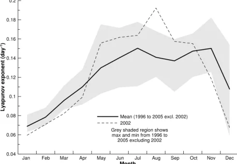
of 2002 (Newman and Nash,2005) appears as a patch of reduced weak mixing dur-ing the 2002 winter at 450 K. At 550 K and 650 K mixdur-ing in late autumn and winter is stronger than usual, and shows an anomalously early transition to even stronger mixing (as shown for 650 K in Fig.4).

In the northern hemisphere the polar vortex is apparent only in some years, e.g.

10

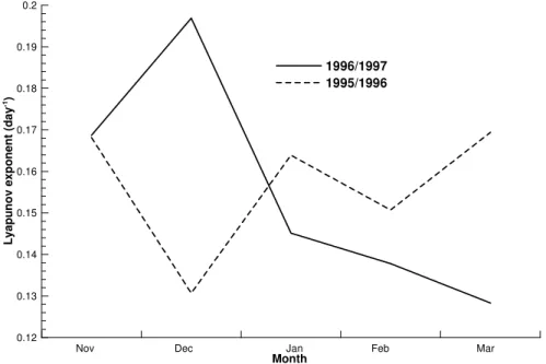
1989/1990, 1996/1997 and 1999/2000 while in other years, e.g. 1984/1985 and 1998/1999, the winter-time mixing extends all the way to the pole. In the Arctic winter of 1996/1997 the vortex did not form until late December after which it was strong and centered on the pole until a late breakdown in April (Coy et al.,1997). This behaviour is apparent at 450 K in Fig.5where a sharp transition from strong mixing in December

15

to weak mixing in January in the Arctic can be seen. This transition is also appar-ent, but less clearly, at 550 K and 650 K (not shown). The opposing seasonal patterns of change in the Arctic winters of 1995/1996 (weak to strong mixing) and 1996/1997 (strong to weak mixing) are reflected in minimum Arctic temperatures on the 475 K surface and in the strength the jet (Figs. 1 and 2 ofCoy et al.,1997).

20

In the tropics, the annual cycle is still apparent but superimposed by interannual differences, especially at upper levels. At 450 K the “tropical reservoir” (Trepte and

Hitchmann,1992), a region of low mixing within ∼15◦ of the equator, is apparent each year with varying strength while at the upper levels, regions of high and low mixing show a more complex structure. At the two upper levels, some two-year periodicity can

25

(14)

ACPD

7, 6189–6228, 2007

Full Screen / Esc

EGU

5 Regression model analysis

5.1 Regression model fits

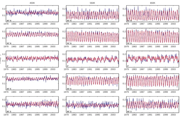
The regression model described in Sect. 3 was applied to the zonal mean monthly Lyapunov exponent time series at each degree of latitude from 1979 to 2005. Examples of regression model fits at 5 selected latitudes and all three analysis levels are shown

5

in Fig.6. At latitudes of 50◦north and south the variability is dominated by the annual cycle and the model captures the variability well (coefficients of multiple determination

R2 as given by Eq. (4) are 0.93, 0.88, 0.93 and 0.92) at the two upper levels. At 450 K in the mid-latitudes the annual cycle is less pronounced, and less variability is explained by the model (R2 values of 0.69 and 0.51). In the polar regions (80◦N/S),

10

at all three levels, the year-to-year variability is much higher and the regression model has difficulty tracking the observations. At 550 K in the northern hemisphere, and at 650 K in both hemispheres, the observed Lyapunov exponents show a strong annual cycle and the regression model captures much of the variance – note however, that the large Arctic winter-time mixing in 1985, 1989, and 2001 is not fully captured by

15

the regression model, suggesting that there are additional sources of variability not currently accounted for. At 550 K in the southern hemisphere, and at 450 K in both hemispheres, the annual cycle is very weak and the regression model has difficulty tracking the observations (R2values of 0.29, 0.48 and 0.36). At the equator, the model fits the variability in the observed Lyapunov exponent time series very well (R2values

20

close to 0.71).

5.2 Lyapunov exponent climatology

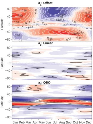
The ai coefficients in Eq. (1) have been expanded at daily resolution (see Eq. 2) at

each latitude and coefficients 1 to 3 are plotted in Figs.7,8 and9 for the three isen-tropic levels. The first coefficient (a1, uppermost panel) represents the climatology in

25

Lyapunov exponents for years 1979–2005 and was significant (ai>2σa_i, see Sect. 3)

(15)

ACPD

7, 6189–6228, 2007

Full Screen / Esc

for all latitudes and times.

The climatology for 450 K shows high winter-time values of Lyapunov exponents in the mid-latitudes of both hemispheres. In the mid-latitudes of the southern hemisphere the annual cycle in mixing is small and values remain high year round with a maxi-mum in spring (September to November) at around 60◦S in approximate agreement

5

withAllen and Nakamura(2001) andHaynes and Shuckburgh(2000). Throughout the northern hemisphere, however, we find weaker mixing in summer than in winter which disagrees with Allen and Nakamura(2001) and Haynes and Shuckburgh(2000) who found strong mixing at 450 K in northern summer.

The tropics are characterized by a broad band of low values from May to November,

10

which is shifted slightly toward the northern hemisphere. From December to April there is a narrow band of low mixing at about 15◦S. This shift toward the summer pole is also apparent in the 18 month time series ofHaynes and Shuckburgh(2000), even though they find a broad band of low mixing year round.

The Antarctic vortex appears as a region of very low Lyapunov exponents with

15

steep gradients across 60◦S. Mixing is low within the vortex, in agreement with

Haynes and Shuckburgh (2000) and Bowman (1993). This strong barrier develops in late autumn (April–June) and remains strong until the vortex breaks up in spring (October–December). The maximum in mixing is located at the vortex edge in Octo-ber/November, which coincides with erosion of the polar vortex by breaking planetary

20

waves. In the Arctic mixing is lowest in summer, and the Arctic vortex is hardly apparent in zonally averaged Lyapunov exponents.

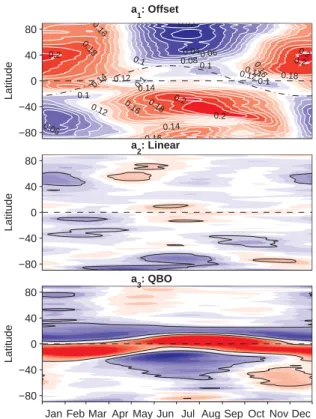
The climatologies at 550 K and 650 K show many similarities. The high mixing in the surf-zone in winter and low mixing in summer mid-latitudes appear at both levels, with a stronger annual cycle at 650 K. Also at both levels the summer minimum extends to

25

the pole in the northern but not in the southern hemisphere. The tropical climatology at these two upper levels shows a seasonally consistent spatial pattern whereby regions of generally low mixing follow a path that is close to, but not perfectly coincident with, the solar declination (dash-dot line in Fig. 8). However, the mixing is not uniform in

(16)

ACPD

7, 6189–6228, 2007

Full Screen / Esc

EGU

time along this path and 5 periods of low mixing are interspersed with periods of higher mixing. In the summer hemisphere, a region of higher mixing occurs equatorward of the regions of low mixing, but appears confined to the tropics and separated from the main winter-time region of high mixing in the mid-latitudes. The pattern at 650 K is similar to the pattern at 550 K but with longer lasting maxima and suppressed minima.

5

Due to the large influence of the QBO in the tropics (see Sect. 5.4), these tropical mixing patterns are unlikely to be directly comparable to other studies which consider only a few years of data and show time series rather than climatologies (e.g.Haynes

and Shuckburgh,2000).

In contrast to 450 K, there are high values of Lyapunov exponents within the fully

10

developed Antarctic vortex in mid-winter. The polar barrier is visible as a band of lower values south of 60◦S. The barrier appears stronger at 550 K than at 650 K and low mixing extends all the way to the pole just before the final warming mixes air from within the vortex into mid-latitudes in early summer. This behavior is again in good agreement withHaynes and Shuckburgh(2000). As at 450 K, the Arctic vortex is seen

15

only weakly.

5.3 Trends in mixing

The a2 coefficients from Eq. (1) have been used to describe global, seasonally de-pendent, long-term (1979–2005) trends in mixing at 450 K, 550 K and 650 K. At 450 K, the dominant pattern is a positive trend in mixing in middle and high southern latitudes

20

with highest values in summer. The maximum total change in mixing of 0.03 day−1over the whole period of 27 years is found at ∼65◦S from mid-September to mid-November, suggesting that mixing across the vortex edge on the 450 K surface has increased over this period. Between 40◦S and 60◦S there are also indications of increases in mixing from January to July. In a confined latitude band close to the equator, positive trends

25

in mixing are seen from May to August.

At 650 K both positive and negative trends in mixing are apparent, and the main features occur also at 550 K in addition to some barely significant trends with little

(17)

ACPD

7, 6189–6228, 2007

Full Screen / Esc

itudinal extent. In the northern surf zone, a total winter-time change of –0.03 day−1 occurs at 650 K over the 1979–2005 period. At 650 K (and less so at 550 K), increases in mixing over northern mid-latitudes occur in late spring and early summer. In con-trast spring-time decreases in southern mid-latitudes are seen. Over southern high latitudes, mixing increases in spring/summer and decreases in winter within the

vor-5

tex. The decreases in winter-time Antarctic mixing are more apparent at 650 K than at 550 K with a total long-term change of –0.05 day−1. In contrast to 450 K, this implies a strengthening of the polar barrier but at an earlier time in the year (July). Over southern high latitudes, increases in mixing are seen at around the time when the vortex breaks up, more so at 550 K than at 650 K.

10

5.4 QBO influence on mixing

The QBO is found to account for most of the non-seasonal variability in Lyapunov exponents in the tropics, as the third panel in Figs.7to9show. The response of mixing to the QBO shows a strong seasonal dependence. Since the QBO basis function is scaled to [-1,1], the parameter a3 added to the climatology a1 corresponds to

west-15

phase conditions (i.e. the QBO panels in the figures show the west phase QBO-induced mixing anomaly and with colour scales reversed would show the east phase mixing anomaly). Recall that the regression model allows for a phase shift in the QBO basis function (see Eq.1). The optimal phase shift, across all latitudes, was found to be –2 months at 450 K, +2 months at 550 K and +6 months at 650 K as expected from the

20

descending nature of the QBO.

In the lower stratosphere, QBO west phases cause mixing to be enhanced around the equator, with the maximum on the summer side of the equator, from June to Octo-ber, accompanied by a decrease in mixing in southern subtropics. During the rest of the year, mixing is inhibited between 5◦S and up to 30◦N. A narrow positive effect is

25

found at 15◦S whereas mixing is lower in the west phase in the southern subtropics year round. At upper levels, the pattern is more seasonally symmetric: in general QBO

(18)

ACPD

7, 6189–6228, 2007

Full Screen / Esc

EGU

parameters at 550 K and 650 K show positive values on the summer side of the equa-tor and negative values on the winter side, though in some cases the winter negative values persist into summer in the sub-tropics.

Shuckburgh et al.(2001) investigated the influence of the QBO on isentropic mixing at 624 K (they argued that the influence is strongest at this level) for 6 years. They

5

found inhibited mixing in east phases throughout the tropics and a narrow band of weak mixing at the equator with regions of enhanced mixing surrounding it during westerly phases. Their calculations were based on equivalent lengths estimated from tracer contours, which were simulated from ECMWF analyzed winds. Our results agree, with a broad region of inhibited mixing close to the equator in easterly phases, but with

10

a seasonal shift of the pattern into the summer hemisphere. Both analyses show a strong maximum in mixing on the summer side of the equator in westerly QBO phases. In contrast toShuckburgh et al.(2001), our analyses show weaker winter-time mixing in the surf zone that does not extend as close to the equator during westerly QBO phases.

15

Over the Arctic, at all three levels (but less so at 650 K), mixing is negatively cor-related with the QBO in winter and positively corcor-related with the QBO in spring. This implies a strengthened Arctic vortex in QBO west phases and a weaker vortex with enhanced mixing in middle to high latitudes in QBO east phases. These results are consistent withHolton and Tan (1980) who showed increased wave activity in winter

20

(November-December) during easterly QBO phases and in late winter/spring (January-March) during westerly QBO phases. This QBO influence on the Antarctic polar vortex is less obvious though the signal at 650 K extends far into the southern hemisphere. 5.5 Solar cycle and ENSO influence on mixing

Both solar cycle and El Ni ˜no Southern Oscillation (ENSO) signals are seldom

statisti-25

cally significant in the Lyapunov exponents at all levels (not shown). The only signif-icant signal that lasts for a few months over a broad range of latitudes is a negative correlation of the ENSO with Lyapunov exponents in spring/early summer in northern

(19)

ACPD

7, 6189–6228, 2007

Full Screen / Esc

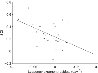
mid-latitudes at 550 K and 650 K. This is shown for 650 K in Fig.10, where Lyapunov exponents, with the offset, the trend, the QBO and the solar cycle signal removed, and averaged over April–June and over 30◦ to 60◦N are plotted against the ENSO index (i.e. the SOI). The correlation between the plotted Lyapunov exponents and SOI is

−0.51, and the correlation is significant at the 99.5% level. The variability in the

aver-5

aged Lyapunov exponent residuals is only partly captured by ENSO/SOI (theR2value, see Eq.4, of the linear fit is 0.26). However, the ENSO signal in other atmospheric

quantities (temperature, ozone) shows strong longitudinal structure (Randel and Cobb,

1994), with the result that the zonal mean analyses presented here may obscure some features. Randel and Cobb (1994) show a wave-1 pattern in winter high latitudes,

10

which coincides with the strongest signal found in mixing. 5.6 Zonal averages over equivalent latitudes

In addition to the zonal averages over geographical latitude, Lyapunov exponents were averaged over latitudes related to potential vorticity (PV) contours i.e. equivalent lati-tude (Butchart and Remsberg,1986). The equivalent latitude of a location with

poten-15

tial vorticity PVloc is the geographic latitude enclosing the same area as the area over which PV exceeds or equals PVloc. The equivalent latitude transformation places the pole at the center of the vortex and, when calculating zonal means, preserves steep meridional gradients in atmospheric constituents that are correlated with PV. Equivalent latitudes were calculated based on NCEP/NCAR reanalysis PV fields.

20

The regression model (Eq.1) was applied to the equivalent latitude averaged Lya-punov exponents, and the variability explained by the model was similar to that for true latitude. The climatologies (coefficient a1) reveal generally steeper gradients of Lyapunov exponents at the vortex edges, both in the Antarctic and the Arctic. The differences were most apparent at 550 K, and the climatology at this level is shown in

25

Fig. 11. The Arctic vortex, which was hardly visible in true latitude coordinates, can be clearly identified as low values in autumn/early winter, extending through the winter with steep gradients at around 60◦N equivalent latitude. In Antarctica, high values at

(20)

ACPD

7, 6189–6228, 2007

Full Screen / Esc

EGU

the vortex edge are concentrated in a narrow band, and with rapid decreases in mixing just equatorward of the vortex edge as the vortex breaks up. The Arctic vortex is appar-ent also at 450 K and 650 K in equivalappar-ent latitudes (not shown). The Antarctic vortex and its barrier to mixing is far more clearly visible in equivalent latitude coordinates than its Arctic counterpart. The regression model coefficients a2toa5show only small

5

differences when averaged over equivalent latitude rather than true latitude.

6 Discussion and conclusions

The analyses presented above show that Lyapunov exponents appear to be a useful diagnostic of stratospheric mixing: they show regions of strong mixing that coincide with the expected regions of the mid-latitude surf zone, barriers to mixing in the

sub-10

tropics and at the polar vortex edge as shown by steep gradients in PV (see Fig.2), and the seasonal climatology in mixing revealed by the Lyapunov exponents agrees well with previous studies (e.g.Haynes and Shuckburgh,2000;Nakamura,1996). Av-eraging over equivalent latitudes showed more clearly the polar barriers, especially in the northern hemisphere where the vortex is highly asymmetric and conventional zonal

15

averaging blurs the steep gradients in mixing.

This study, one of the first to present multi-decadal time series of stratospheric mix-ing, shows long-term secular trends in mixmix-ing, interannual variability on time scales coincident with main sources of atmospheric variability e.g. the QBO, as well as un-explained variability (“noise”) whose magnitude varies with latitude and altitude.

Es-20

pecially in the tropics and subtropics, mixing is strongly modulated by the QBO, with a strong seasonal dependence. To show the QBO modulation of mixing more clearly, latitude-potential temperature cross-sections in July for two indicative years with oppo-site QBO phases are shown in Fig.12 together with monthly mean zonal mean zonal winds.

25

For July 1997, when the equatorial zonal winds were westerly, the region of en-hanced mixing in the summer tropics/subtropics coincides with the zero wind line. This

(21)

ACPD

7, 6189–6228, 2007

Full Screen / Esc

agrees withShuckburgh et al. (2001) and suggests that in QBO west phases, plane-tary waves can penetrate from the winter hemisphere into the tropics and break on the summer side of the equator (where winds turn easterly), which is expected to increase mixing there. In July 1984, when zonal winds are easterly throughout the tropics and the zero wind line lies at around 20◦S, planetary waves are expected to break on the

5

winter side of the tropics, which explains the higher mixing in the winter subtropics. The consistency of this behaviour with variability in wave activity is shown in Fig.13

where 50 hPa July monthly mean zonal mean eddy heat fluxes (v′_T′_{) for southern low} latitudes are shown for different phases of the QBO.

It can be seen that in east phases, v ′_T′

exceeds the mean values whereas in west

10 phases v ′_T′

is weaker than usual south of 15 ◦

S, as expected from the discussion above. However, even though it is assumed that planetary wave breaking is the main cause of mixing, further analyses is required to explore the relationship between plan-etary wave breaking and mixing diagnostics (in particular Lyapunov exponents), and to determine which other factors contribute to dynamical mixing.

15

The QBO induced variability in mixing is likely to have an influence on the distribu-tion of long-lived atmospheric trace gases such as ozone. During QBO west phases, a strengthened tropical barrier on the winter side of the equator and enhanced mixing in the summer tropics/subtropics suggests that trace gases, whose source is in the trop-ics, should show a positive anomaly in the summer subtropics and a negative anomaly

20

in the winter hemisphere. However, because the effect of the QBO on mixing is sea-sonally dependent, the anomaly in trace gas distributions is sensitive to the phasing of the QBO with respect to the annual cycle. The effects of this phasing on southern mid-latitude total column ozone have been analyzed by Bodeker et al. (2007)1. The suggestion of penetration of planetary waves across the equator (Shuckburgh et al.,

25

2001, see discussion above) is in agreement with net transport from the winter

hemi-1

Bodeker, G. E. Garny, H., Smale, D., Dameris, M., and Deckert, R.: The 1985 southern hemisphere mid-latitude total column ozone anomaly, Atmos. Chem. Phys., submitted, 2007

(22)

ACPD

7, 6189–6228, 2007

Full Screen / Esc

EGU

sphere into the summer hemisphere as suggested here and in Bodeker et al. (2007)1. A QBO signal in mixing could be identified in northern high-latitudes (strongest at 550 K), with decreased mixing in winter and increased mixing in spring during QBO west phases, suggesting a strengthened Arctic vortex in west QBO conditions. As mentioned earlier, this behaviour is consistent withHolton and Tan(1980) and

follow-5

up studies (Dunkerton and Baldwin,1991;Dameris and Ebel,1990). The mechanism suggested byHolton and Tan(1980) is a narrowed wave guide for planetary waves in QBO east phases, causing the wave activity to increase in middle to high latitudes. In-creased wave activity and the narrowed wave guide increases the Eliassen-Palm (EP) flux (Randel et al.,1987) towards high latitudes, strengthening the wave-driven mean

10

meridional circulation and causing increased subsidence at high latitudes so that the overall effect is to weaken the vortex in east phases. Our results show increased mix-ing for east phases from the equator to about 30◦N and for latitudes higher than 55◦N in mid-winter. From the Holton-Tan mechanism, increased wave activity is expected at mid-latitudes, and since mixing occurs where waves break, the regions of increased

15

mixing over high latitudes supports the concept of enhanced erosion of the polar vortex by planetary wave breaking.Ruzmaikin et al.(2005) calculated differences in EP fluxes carried by wave 1 and wave 2 for west and east phases of the QBO from NCEP/NCAR reanalyses data at 20 hPa and found significantly higher fluxes for wave 1 in early win-ter (October–December) and lower fluxes in late winwin-ter/spring (January–February) in

20

east phases. Significant differences in wave 2 fluxes were found in spring (February– March), where fluxes are lower in east phases than in west phases. The change of sign in the difference in wave fluxes (east minus west) from winter to spring compares well to the change of sign in mixing anomalies found here.

In the southern hemisphere, no significant QBO signal in mixing could be detected at

25

high latitudes. However, at 650 K (and less so at 550 K), in winter, the QBO signal ex-tends far into the mid-latitudes (60◦S) and in spring/early summer a positive correlation is found. If the wave activity in the southern hemisphere is modulated as suggested by the Holton-Tan mechanism (increased wave activity in east phases), the

(23)

ACPD

7, 6189–6228, 2007

Full Screen / Esc

tion of mixing in the mid-latitudes rather than at high latitudes suggests that the waves break at lower latitudes than in the northern hemisphere. A possible explanation is the comparably stronger polar vortex over Antarctica, causing waves to break at its edge and not, as in the northern hemisphere, propagate to high latitudes and break there. Our analyses of eddy heat fluxes at 30 hPa for July (not shown) suggest that values of

5

v′_T′_{averaged over years with QBO west phases are lower than values of}_v′_T′ _{in QBO} easterlies between 40◦S and 70◦S (at 60◦S eddy heat fluxes in QBO westerlies are about one third of eddy heat flux values in QBO easterlies). This finding supports the hypothesis of enhanced erosion of the polar vortex in QBO east phases.

The regression analysis applied to monthly zonal mean Lyapunov exponents

re-10

vealed trends in mixing over the analysis period of 27 years. At 450 K, an increase in mixing in the southern hemisphere, mainly in late winter/spring, is the main feature and holds also for shorter analysis periods (e.g. 1979–2000 and 1985–2005), which were calculated to test the sensitivity of the trend to different analysis periods. This trend is consistent with an increase in winter-time wave 1 amplitudes at 60◦S over the same

15

time period (Bodeker et al., 20071). From 1979 to 2005 zonal winds at 450 K and 60◦S in October show a positive trend (see Fig.14).

Zonal mean zonal winds at 450 K and 60◦S in October were correlated with Lya-punov exponents from which all fitted signals, other than the trend, were removed. It was found that the best correlation is obtained with averages over 60◦–80◦S in August

20

(correlation coefficient −0.68, significant at the 99.5% level). The negative correlation between August Lyapunov exponents and October zonal winds, apparent in Fig. 14, is at odds with the long-term positive trend in both quantities. This suggests that dif-ferent mechanism drive the year-to-year and long-term interactions between Lyapunov exponents and vortex strength.

25

The negative correlation on short time scales is likely to be due to increased wave activity enhancing the wave-driven mean meridional circulation which increases sub-sidence and therefore the temperature at high latitudes and so decreases the vor-tex strength (as found by Newman et al., 2001, for the northern hemisphere). This

(24)

ACPD

7, 6189–6228, 2007

Full Screen / Esc

EGU

mechanism therefore represents a response of the vortex strength to mostly unex-plained variability in wave driving (the correlation between Lyapunov exponents and zonal winds proves to be even higher when taking only the residual term into account). The long-term trend in the 60◦S zonal winds is believed to be caused by decreasing po-lar temperatures due to ozone depletion (Thompson and Solomon,2002). Therefore,

5

in contrast to the proposed short-term mechanism where mixing influences the vortex strength, on longer time scales the change in zonal winds is likely to influence mixing. Since Lyapunov exponents do not directly measure wave activity, but rather shear and strain rates, higher wave activity will result not only in higher Lyapunov exponents but also higher shear due to a stronger polar jet. This again highlights the need to explore

10

the physical causes of mixing in more detail.

The trends at 550 K and 650 K are consistent with a strengthening of the Antarctic vortex, with decreased mixing in winter at high latitudes and increased mixing in spring. Mixing at the vortex edge is highly correlated with wave activity, quantified here as eddy heat flux (the correlation coefficient for 650 K Lyapunov exponents with 30 hPa eddy

15

heat flux at 60◦S is −0.75). The winter/early spring decrease in northern mid-latitude

mixing is consistent with the changes in EP fluxes noted byHadjinicolaou et al.(2005). Acknowledgements. We would like to thank C.-F. Shih at the National Center for Atmospheric

Research and the National Centers for Environmental Prediction for the NCEP/NCAR data. H. Garny was funded through the Deutsche Akademische Austauschdienst (DAAD). This work

20

was conducted within the FRST funded Drivers and Mitigation of Global Change programme (C01X0204).

References

Allen, D. R. and Nakamura, N.: A seasonal climatology of effective diffusivity in the strato-sphere, J. Geophys. Res., 106, 7917–7936, 2001. 6191,6192,6202

25

Bowman, K.: Large-scale isentropic mixing properties of the Antarctic polar vortex from ana-lyzed winds, J. Geophys. Res., 98, 23 013–23 027, 1993.6191,6192,6193,6195,6202

(25)

ACPD

7, 6189–6228, 2007

Full Screen / Esc

Printer-friendly Version Interactive Discussion Butchart, N. and Remsberg, E. E.: The area of the stratospheric polar vortex as a diagnostic

for tracer transport on an isentropic surface, J. Atmos. Sci., 43(13), 1319–1339, 1986. 6206

Coy, L., Nash, E. R., and Newman, P. A.: Meteorology of the polar vortex: Spring 1997, Geo-phys. Res. Lett., 24(22), 2693–2696, 1997. 6200

Dameris, M. and Ebel, A.: The quasi-biennial oscillation and major stratospheric warmings - A

5

three-dimensional model study, Ann. Geophys., 8, 79–85, 1990,

http://www.ann-geophys.net/8/79/1990/. 6209

Dunkerton, T. J. and Baldwin, M. P.: Quasi-biennial modulation of planetary-wave fluxes in the northern hemisphere winter, J. Atmos. Sci., 48(8), 1043–1061, 1991. 6209

Hadjinicolaou, P., Pyle, J. A., and Harris, N. R. P.: The recent turnaround in stratospheric ozone

10

over northern middle latitudes: A dynamical modeling perspective, Geophys. Res. Lett., 32, L12821, doi:10.1029/2005GL022476, 2005. 6211

Haynes, P. and Shuckburgh, E.: Effective diffusivity as a diagnostic of atmospheric transport 1. Stratosphere, J. Geophys. Res., 105, 22 777–22 794, 2000. 6191,6192,6194,6202,6203,

6207

15

Holton, J. R. and Tan, H.-C.: The influence of the equatorial quasibiennial oscillation on the global circulation at 50 mb, J. Atmos. Sci., 37, 2200–2208, 1980. 6205,6209

Hood, L., Rossi, S., and Beulen, M.: Trends in lower stratospheric zonal winds, Rossby wave breaking behaviour, and column ozone at northern midlatitudes, J. Geophys. Res., 104(D20), 24 321–24 339, 1999. 6191

20

Hoskins, B. J., McIntyre, M. E., and Robertson, A. W.: On the use and significance of isentropic potential vorticity maps, Q. J. R. Meteorol. Soc., 111, 877–946, 1985. 6191

Kalnay, E., Kanamitsu, M., Kistler, R., Collins, W., Deaven, D., Gandin, L., Iredell, M., Saha, S., White, G., Woollen, J., Zhu, Y., Leetmaa, A., Reynolds, B., Chelliah, M., Ebisuzaki, W., Higgins, W., Janowiak, J., Mo, K. C., Ropelewski, C., Wang, J., Jenne, R., and Joseph, D.:

25

The NCEP/NCAR 40-Year Reanalysis Project, Bull. Am. Soc., 77(3), 437–472, 1996.6195

McIntyre, M. and Palmer, T.: The “surf zone” in the stratosphere, J. Atmos. Terr. Phys., 46, 825–849, 1984. 6191,6192

McKenna, D., Konopka, P., Grooß, J.-U., G ¨unther, G., and M ¨uller, R.: A new Chemical La-grangian Model of the Stratosphere (CLaMS) 1. Formulation of advection and mixing, J.

30

Geophys. Res., 107, 4332, doi:10.1029/2000JD000114, 2002. 6191,6194

Nakamura, N.: Two-dimensional mixing, edge formation, and permeability diagnosed in an area coordinate, J. Atmos. Sci., 53(11), 1524–1537, 1996. 6191,6207

(26)

ACPD

7, 6189–6228, 2007

Full Screen / Esc

EGU Nakamura, N. and Ma, J.: Modified Lagrangian-mean diagnostics of the stratospheric polar

vortices 2. Nitrous oxide and seasonal barrier migration in the cryogenic limb array etalon spectrometer and SKYHI general circulation model, J. Geophys. Res., 102(D22), 25 721– 25 735, 1997.6191

Newman, P. A., Nash, E. R., and Rosenfield, J. E.: What controls the temperature of the Arctic

5

stratosphere during the spring?, J. Geophys. Res., 106 (D17), 19 999–20 010, 2001. 6210

Newman, P. A. and Nash, E. R.: The Unusual Southern Hemisphere Stratosphere Winter of 2002, J. Atmos. Sci., 62, 614–628, 2005. 6200

Pierrehumbert, R. T. and Yang, H.: Global Chaotic Mixing on Isentropic Surfaces, J. Atmos. Sci., 50, 2462–2480, 1993.6191,6193

10

Plumb, R. A. and Ko, M. K. W.: Interrelationships between mixing ratios of long-lived strato-spheric constituents, J. Geophys. Res., 97(D9), 10 145–10 156, 1992. 6191

Press, W. H., Flannery, B. P., Teukolsky, S. A., and Vetterling, W. T.: Numerical recipes in Pascal. The art of scientific computing, Cambridge University Press, 1989. 6193

Randel, W. J., Stevens, D. E., and Stanford, J. L.: A study of planetary waves in the southern

15

winter troposphere and stratosphere. Part II: Life cycles, J. Atmos. Sci., 44(6), 936–949, 1987. 6209

Randel, W. and Cobb, J.: Coherent variations of monthly mean total ozone and lower strato-spheric temperature, J. Geophys. Res., 99, 5433–5447, 1994. 6206

Randel, W. J., Wu, F., and Stolarski, R.: Changes in column ozone correlated with the

strato-20

spheric EP flux, J. Meteorol. Soc. Japan, 80, 849–862, 2002.6191

Ruzmaikin, A., Feynman, J., Jiang, X., and Yung, Y.L.: Extratropical signature of the quasi-biennial oscillation, J. Geophys. Res., 110, D11111, doi:10.1029/2004JD005382, 2005.6209

Shuckburgh, E. and Haynes, P.: Diagnosing transport and mixing using a tracer-based coordi-nate system, Physics of Fluids, 15, 3342–3357, 2003. 6194

25

Shuckburgh, E., Norton, W., Iwi, A., and Haynes, P.: Influence of the quasi-biennial oscillation on isentropic transport and mixing in the tropics and subtropics, J. Geophys. Res., 106, 14 327–14 337, 2001. 6191,6192,6198,6205,6208

Tan, D. G. H., Haynes, P. H., MacKenzie, A. R., and Pyle, J. A.: Effects of fluid-dynamical stirring and mixing on the deactivation of stratospheric chlorine, J. Geophys. Res., 103(D1),

30

1585–1605, 1998. 6192

Thompson, D. W. J. and Solomon, S.: Interpretation of recent southern hemisphere climate change, Science, 296, 895–899, 2002. 6211

(27)

ACPD

7, 6189–6228, 2007

Full Screen / Esc

Printer-friendly Version Interactive Discussion Tiao, G., Reinsel, G., Xu, D., Pedrick, J., Zhu, X., Miller, A., DeLuisi, J., Mateer, C., and

Wueb-bles, D.: Effects of autocorrelation and temporal sampling schemes on estimates of trend and spatial correlation, J. Geophys. Res., 95(D12), 20 507–20 517, 1990. 6197

Trepte, C. R. and Hitchman, M. H.: Tropical stratospheric circulation deduced from satellite aerosol data, Nature, 355, 626–628, 1992.6192,6200

5

van Loon, H. and Labitzke, K.: The Influence of the 11-year Solar Cycle on the Stratosphere Below 30 km: a Review, Space Science Reviews, 94, 259–278, 2000. 6198

von Storch, H. and Zwiers, F. W.: Statistical Analysis in Climate Research, Statistical Anal-ysis in Climate Research, by Hans von Storch and Francis W. Zwiers, pp. 494. ISBN 0521012309. Cambridge, UK: Cambridge University Press, 2002. 6196,6198

10

Waugh, D. W.: Subtropical stratospheric mixing linked to disturbances in the polar vortices, Nature, 365, 535–537, 1993. 6191,6192

Waugh, D., Plumb, R., Atkinson, R. J., Schoeberl, M. R., Lait, L. R., Newman, P. A., Loewen-stein, M., Toohet, D., Avallone, L., Webster, C., and May, R.: Transport out of the lower stratospheric vortex by Rossby wave breaking, J. Geophys. Res., 99(D1), 1071–1088, 1994.

15

6191

Wolf, A., Swift, J. B., Swinney, H. L., and Vastano, J. A.: Determining Lyapunov exponents from a time series, Physica D Nonlinear Phenomena, 16, 285–317, 1985.6193,6194,6195

(28)

ACPD

7, 6189–6228, 2007

Full Screen / Esc

Printer-friendly Version Interactive Discussion EGU 80oS 60o_S 40o_S start A B

Fig. 1. Trajectories (red and green solid line) for a 12 day period on the 450 K level,

commenc-ing on 1 August 2000, and with renormalization after 6 days (A and B). The distances A and B, shown as dashed lines, are used to calculate Lyapunov exponents. To show more clearly the evolving spatial separation of the trajectories, the distance between the starting points has been set at 100 km compared to the 1 km value used in the calculations presented in this paper.

(29)

ACPD

7, 6189–6228, 2007

Full Screen / Esc

Printer-friendly Version Interactive Discussion February 1997 , 550K 150 oW 120 oW 90 o W 60 o W 30o W 0o 30 oE 60 oE 90 oE 120 o E 150 o E 180o_W February 1989 , 550K 150 oW 120 oW 90 o W 60 o W 30 o W 0o 30 oE 60 oE 90 oE 120 o E 150 o E 180o W August 1989 , 550K 150 o W 120 o W 90 o W 60 oW 30 oW 0o 30 o E 60 o E 90 oE 120 oE 150 oE 180o W August 2002 , 550K 150 o W 120 o W 90 o W 60 oW 30 oW 0o 30o E 60 o E 90 oE 120 oE 150 oE 180o W 0.02 0.04 0.06 0.08 0.1 0.12 0.14 0.16 0.18 Lyapunov Exponents (day−1

)

Fig. 2. Example Lyapunov exponents for February in the northern hemisphere (upper panels)

and for August in the southern hemisphere (lower panels), on the 550 K surface. For each hemisphere, results from two years are presented and compared. Regions coloured red show high mixing while regions coloured blue show low mixing. Overlaid on the Lyapunov distribu-tions are the 550 K PV fields, shown as contour plots, at the start time of the trajectories used

(30)

ACPD

7, 6189–6228, 2007

Full Screen / Esc

EGU

Lyapunov Exponent at 450K [1/day] 0.07 0.09 0.11 0.13 0.15 0.17 Latitude 1980 1982 1984 1986 1988 1990 1992 1994 1996 1998 2000 2002 2004 2006 −80 −60 −40 −20 0 20 40 60 80

Lyapunov Exponent at 550K [1/day] 0.03 0.05 0.07 0.09 0.11 0.13 0.15 0.17 Latitude 1980 1982 1984 1986 1988 1990 1992 1994 1996 1998 2000 2002 2004 2006 −80 −60 −40 −20 0 20 40 60 80

Lyapunov Exponent at 650K [1/day]

0.02 0.04 0.06 0.08 0.1 0.12 0.14 0.16 0.18 0.2 Latitude 1980 1982 1984 1986 1988 1990 1992 1994 1996 1998 2000 2002 2004 2006 −80 −60 −40 −20 0 20 40 60 80

Fig. 3. Zonally averaged Lyapunov Exponents for 650 K (top), 550 K (middle) and 450 K

(bot-tom) for years 1979–2005. Note the different colour scales.

(31)

ACPD

7, 6189–6228, 2007

Full Screen / Esc

Jan Feb Mar Apr May Jun Jul Aug Sep Oct Nov Dec

Month 0.04 0.06 0.08 0.1 0.12 0.14 0.16 0.18 0.2 L y a p u n o v e x p o n e n t (d a y -1) Mean (1996 to 2005 excl. 2002) 2002

Grey shaded region shows max and min from 1996 to

2005 excluding 2002

Fig. 4. Lyapunov exponents averaged over 60◦S to 90◦S at 650 K for 2002 (dashed line). The

10-year mean 1996 to 2005 (excluding 2002) is shown as a solid line together with the range of values over this time period (grey shaded region).

(32)

ACPD

7, 6189–6228, 2007

Full Screen / Esc

Printer-friendly Version Interactive Discussion EGU Month 0.12 0.13 0.14 0.15 0.16 0.17 0.18 0.19 0.2 L y a p u n o v e x p o n e n t (d a y -1) 1996/1997 1995/1996

Nov Dec Jan Feb Mar

Fig. 5. Lyapunov exponents averaged over 60◦N to 90◦N at 450 K for the northern winters

1995/96 (dashed line) and 1996/97 (solid line).

(33)

ACPD

7, 6189–6228, 2007

Full Screen / Esc

Printer-friendly Version Interactive Discussion 1979 1983 1987 1991 1995 1999 2003 0.1 0.2 80° S 1979 1983 1987 1991 1995 1999 2003 0.1 0.2 50° S 1979 1983 1987 1991 1995 1999 2003 0.1 0.2 λ (day −1 ) 0° 1979 1983 1987 1991 1995 1999 2003 0.1 0.2 50° N 1979 1983 1987 1991 1995 1999 2003 0.1 0.2 450K 80° N 1979 1983 1987 1991 1995 1999 2003 0.1 0.2 80° S 1979 1983 1987 1991 1995 1999 2003 0.1 0.2 50° S 1979 1983 1987 1991 1995 1999 2003 0.1 0.2 0° 1979 1983 1987 1991 1995 1999 2003 0.1 0.2 50° N 1979 1983 1987 1991 1995 1999 2003 0.1 0.2 550K 80° N 1979 1983 1987 1991 1995 1999 2003 0.1 0.2 80° S 1979 1983 1987 1991 1995 1999 2003 0.1 0.2 50° S 1979 1983 1987 1991 1995 1999 2003 0.1 0.2 0° 1979 1983 1987 1991 1995 1999 2003 0.1 0.2 50° N 1979 1983 1987 1991 1995 1999 2003 0.1 0.2 650K 80° N

Fig. 6. Time series of calculated (blue) and modelled (red) Lyapunov Exponents for latitudes

80◦N/S, 50◦N/S, and the equator. Left panels show regression model fits for 450 K, middle panels for 550 K and right panels for 650 K.

(34)

ACPD

7, 6189–6228, 2007

Full Screen / Esc

Printer-friendly Version Interactive Discussion EGU 0. 12 0.14 0.14 0.14 0. 14 0.16 0.16 0.16 0.12 0.16 0.12 0.18 0.18 0.18 0.16 0.1 0. 18 0.1 0.18 0.18 Latitude −80 −40 0 40 80 Latitude −80 −40 0 40 80

Jan Feb Mar Apr May Jun Jul Aug Sep Oct Nov Dec

Latitude −80 −40 0 40 80 −0.04 −0.02 0 0.02 0.04 Coefficients a₂ and a₃ a 1: Offset a 2: Linear a₃: QBO

Fig. 7. Regression model coefficients at 450 K as given by Eq. (2) but evaluated daily. The

uppermost panel shows the climatology of mixing (a₁), with values indicated by the contour labels. The dash-dotted line denotes the solar declination. For the two lower panels, showing the coefficients of the linear term (a2) and the QBO term (a3), the colour bar at the bottom shows the scaling. Parameters are significant (a_i>2σ_a

i, see text) within the black contours.