HAL Id: hal-00492476
https://hal.archives-ouvertes.fr/hal-00492476
Submitted on 8 May 2015
HAL is a multi-disciplinary open access
archive for the deposit and dissemination of
sci-entific research documents, whether they are
pub-lished or not. The documents may come from
teaching and research institutions in France or
abroad, or from public or private research centers.
L’archive ouverte pluridisciplinaire HAL, est
destinée au dépôt et à la diffusion de documents
scientifiques de niveau recherche, publiés ou non,
émanant des établissements d’enseignement et de
recherche français ou étrangers, des laboratoires
publics ou privés.
Spatial, temporal, and vertical variability of polar
stratospheric ozone loss in the Arctic winters
2004/05-2009/10
Jayanarayanan Kuttippurath, Sophie Godin-Beekmann, Franck Lefèvre,
Florence Goutail
To cite this version:
Jayanarayanan Kuttippurath, Sophie Godin-Beekmann, Franck Lefèvre, Florence Goutail. Spatial,
temporal, and vertical variability of polar stratospheric ozone loss in the Arctic winters
2004/05-2009/10. Atmospheric Chemistry and Physics, European Geosciences Union, 2010, 10 (20),
pp.9915-9930. �10.5194/acp-10-9915-2010�. �hal-00492476�
www.atmos-chem-phys.net/10/9915/2010/ doi:10.5194/acp-10-9915-2010
© Author(s) 2010. CC Attribution 3.0 License.
Chemistry
and Physics
Spatial, temporal, and vertical variability of polar stratospheric
ozone loss in the Arctic winters 2004/2005–2009/2010
J. Kuttippurath, S. Godin-Beekmann, F. Lef`evre, and F. Goutail
UPMC Universit´e Paris 06, Universit´e Versailles-Saint-Quentin, UMR 8190 LATMOS-IPSL, CNRS/INSU, Paris, France Received: 10 May 2010 – Published in Atmos. Chem. Phys. Discuss.: 15 June 2010
Revised: 5 October 2010 – Accepted: 8 October 2010 – Published: 20 October 2010
Abstract. The polar stratospheric ozone loss during the
Arctic winters 2004/2005–2009/2010 is investigated by us-ing high resolution simulations from the chemical trans-port model Mimosa-Chim and observations from Aura Mi-crowave Limb Sounder (MLS), by applying the passive tracer technique. The winter 2004/2005 shows the coldest temperatures, highest area of polar stratospheric clouds and strongest chlorine activation in 2004/2005–2009/2010. The ozone loss diagnosed from both simulations and measure-ments inside the polar vortex at 475 K ranges from 0.7 ppmv in the warm winter 2005/2006 to 1.5–1.7 ppmv in the cold winter 2004/2005. Halogenated (chlorine and bromine) cat-alytic cycles contribute to 75–90% of the ozone loss at this level. At 675 K the lowest loss of 0.3–0.5 ppmv is computed in 2008/2009, and the highest loss of 1.3 ppmv is estimated in 2006/2007 by the model and in 2004/2005 by MLS. Most of the ozone loss (60–75%) at this level results from nitro-gen catalytic cycles rather than halonitro-gen cycles. At both 475 and 675 K levels the simulated ozone and ozone loss evolu-tion inside the vortex is in reasonably good agreement with the MLS observations. The ozone partial column loss in 350–850 K deduced from the model calculations at the MLS sampling locations inside the polar vortex ranges between 43 DU in 2005/2006 and 109 DU in 2004/2005, while those derived from the MLS observations range between 26 DU and 115 DU for the same winters. The partial column ozone depletion derived in that vertical range is larger than that esti-mated in 350–550 K by 19±7 DU on average, mainly due to NOxchemistry. The column ozone loss estimates from both
Mimosa-Chim and MLS in 350–850 K are generally in good agreement with those derived from ground-based ultraviolet-visible spectrometer total ozone observations for the respec-tive winters, except in 2010.
Correspondence to: J. Kuttippurath
1 Introduction
Unlike in the Antarctic winter stratosphere, the chemical ozone loss in the Arctic is highly variable. This variability is primarily caused by the variations in Arctic meteorology. That is, the Arctic stratosphere is often disturbed by plane-tary wave forcing triggered by mountain orography that dis-rupts the unstable polar vortex in most winters. Therefore, the Arctic experiences high extreme cold as well as sudden stratospheric warmings (SSWs) at times. As a result the de-gree of ozone loss is mostly controlled by the strength of the vortex and magnitude of air temperature within. For in-stance, the winters 1995, 1996, 2000, and 2005 were very cold and the cumulative total ozone loss was as high as ∼25– 35% (Rex et al., 2006; WMO, 2007; Goutail et al., 2005). On the other-hand, the winters 1997, 1998, 1999, 2001, 2002, 2006, and 2009 were relatively warm and the loss was mini-mal, about 10–15%, while the winters 2003, 2007, and 2008 were moderately cold and hence, the loss was in an average scale of about 15–20% (WMO, 2007; Goutail et al., 2010).
Significant improvements have been made in understand-ing the chemistry of ozone loss in the polar lower strato-sphere in the last decade. Studies suggest that very low temperatures (<195 K) initiate the formation of Polar Strato-spheric Clouds (PSCs), and chlorine activation on these PSCs triggers the ozone depletion when the sun returns over the Arctic in spring. The halogen cycles ClO–ClO and BrO– ClO contribute about 80–90% of ozone loss in this region through the above-said processes (WMO, 2007). However, ozone loss at higher altitudes is driven by different chemical cycles than those discussed in the lower stratosphere. A de-tailed study on the ozone loss process at higher altitudes is still lacking. The available studies deal with specific issues of mid-winter warming and concomitant mid-latitude ozone loss (for e.g. Grooß et al., 2005a; Vogel et al., 2008). None of these studies perform a detailed analysis of the winter strato-sphere in different conditions to diagnose the contribution
of relevant cycles to the ozone loss in a concluding manner. Although the study by Konopka et al. (2007) deal with more than one winter, it is limited to a box model rather than a full-chemistry three dimensional model. Therefore, a compre-hensive study is warranted on the subject to characterise the contribution of various chemical cycles in the polar strato-sphere in different meteorological conditions. The recent six winters were entirely different in this regard, which provide a perfect platform to perform such a study. So in this paper, we examine the ozone loss and its driving chemical cycles (up to 850 K isentropic level) for the recent winters 2005–2010 and assess the variability of ozone loss in a quantitative perspec-tive using simulations and measurements. Calculations using a high resolution chemical transport model (CTM) together with satellite observations are exploited for this purpose.
The article is organised as follows: After Introduction, the model, measurements and meteorological situation of the studied winters are presented in Sect. 2–4. The simulations of ozone, ozone loss, chlorine monoxide (ClO) and their comparison with observations for the recent winters are de-scribed in Sect. 5. The simulated ozone loss and production rates, contribution of different chemical cycles to the ozone loss and the ozone column loss during the winters are anal-ysed in Sect. 6. Section 7 briefs the conclusion of the study.
2 The simulations with Mimosa-Chim CTM
The Mimosa-Chim CTM has been successfully used for the diagnosis of polar ozone loss in previous winters (Kuttippu-rath et al., 2009; Tripathi et al., 2007, 2006) and is described in detail in Tripathi et al. (2006). The model combines the Mimosa advection code (Hauchecorne et al., 2002) with the REPROBUS chemistry scheme (Lef`evre et al., 1994). The model has a horizontal resolution of 1◦×1◦. It has isen-tropic vertical coordinates on 25 levels, resolved by 5 K in the lower stratosphere. Winds and temperatures are taken from the European Centre for Medium Range Weather Fore-casts (ECMWF) operational analyses. The diabatic transport through the isentropes is computed from the heating rate cal-culations by MIDRAD (Shine, 1987), driven by climatolog-ical H2O, CO2and by the O3fields calculated by
Mimosa-Chim.
The model includes a comprehensive description of strato-spheric chemistry. Absorption cross-sections and kinetics data are based on Sander et al. (2006). The absorption cross-sections of Cl2O2 are taken from Burkholder et al. (1990)
and are extrapolated to 450 nm. They are in very good agree-ment with the most recent Cl2O2spectrum measurements by
Papanastasiou et al. (2009). Monthly varying H2SO4fields
leading to the formation of liquid aerosols in the CTM are computed from the outputs of a 2-D-model long-term sim-ulation, which considers the impacts of volcanic eruptions. The heterogeneous chemistry contains reactions on binary and ternary liquid aerosols, nitric acid trihydrate (NAT), and
0.2 0.2 0.2 0.2 0.2 0.6 0.6 0.6 1 1 1 1 1 1 1.4 2005 400 500 600 0.2 0.2 0.2 0.2 0.6 0.6 2006 400 500 600 0.2 0.2 0.2 0.2 0.6 0.6 0.6 1 1 2007 Potential Temperature (K) 400 500 600 0.2 0.2 0.2 0.2 0.2 0.2 0.6 0.6 0.6 0.6 0.6 1 1 1 1 1.4 2008 400 500 600 0.2 0.2 0.2 0.2 0.6 0.6 0.6 1 1 2009 400 500 600 0.2 0.4 0.6 0.8 1 1.2 1.4 1.6 1.8 Day of year 0.2 0.2 0.6 0.6 1 1 1 2010 −30 0 30 60 90 400 500 600 × 107 Km2 Mar Feb Jan Dec
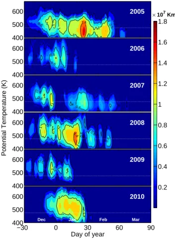
Fig. 1. The area (km2) covered by PSCs (between 400 and 675 K)
inferred from the ECMWF temperature data for the Arctic winters 2005–2010. PSCs are assumed to form at the NAT frost point. The dotted line represents the 475 K and the topmost boundary stands for 675 K potential temperature level.
on water-ice particles. The composition of liquid aerosols is calculated analytically (Luo et al., 1995). The ice particles are assumed to incorporate HNO3 in the form of NAT
de-scribed by a bimodal size distribution (Davies et al., 2002). Cly and Bry are explicitly calculated from their long-lived
sources at the surface and are therefore time dependent. An additional 6 pptv of bromine in the form of CH2Br2is added
to Bryto represent the contribution of brominated short lived
species reaching the stratosphere (WMO, 2007).
For each Arctic winter considered here, the model was run from 1 December to 31 March. Initialisation of ozone on 1 December was provided by the ECMWF operational anal-yses. Other species in Mimosa-Chim were initialised from a long-term simulation of the REPROBUS CTM driven by ECMWF meteorological analyses.
1 1.52 2.5 3 3.54 4.5 4.5 5 5 6 Mimosa−Chim Ozone 400 600 800 1 1.52 2.53 3.5 4 4.5 5 6 Aura MLS Ozone 2005 0 0 0 0.4 Difference (Model−MLS) 11.5 2 2.5 33.5 4 4.5 5 400 600 800 1 1.5 22.5 3 3.5 4 5 2006 −0.4 0 0 0.4 0.4 0.4 1 1.52.52 3 3.5 4 4 4.5 5 Potential Temperature (K) 400 600 800 1 1.52 2.53 3.5 4 4.5 5 2007 −0.8 −0.4 0 0 0 0 0 0 0 1 1.52 2.5 3 3.54 4 4.55 5.5 6 400 600 800 1 1.52 2.5 3 3.54 4.5 4.55 5.5 6 2008 −0.8 −0.4 0 0 0.4 0.4 1 1.5 2 2.5 3 3.5 4 5 400 600 800 1 1.522.5 3 3.5 4 4.5 5 2009 −0.8 −0.4 0 0 0 0 1 1.5 2 2.53 3.5 4 4.5 5 5 5.5 6 −30 0 30 60 90 400 600 800 Day of year 1 1.5 2 2.5 3 3.5 4 4.5 4.5 5 5.5 6 2010 0 30 60 90 1 2 3 4 5 6 7 0 0 0 0 0 0 0.4 0.4 0 30 60 90 −0.5 0 0.5
Jan Feb Mar
Dec Jan Feb Mar Dec Jan Feb Mar
ppmv ppmv
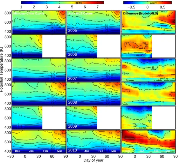
Fig. 2. Temporal evolution of the vertical distribution (350–850 K) of vortex averaged (≥65◦EqL) ozone (ppmv) for the Arctic winters
2005–2010. Left: Mimosa-Chim calculations, Middle: MLS measurements, and Right: The difference between modelled and measured ozone. The model fields are sampled at location of the MLS observations. Due to early vortex dissipation caused by major warmings, the analysis does not extend beyond 10 February in 2006 and 2009. Both data are smoothed for seven days. The white dotted lines represent the study altitudes 475 and 675 K.
3 Measurements: Aura MLS
Ozone and ClO observations (version 2.2) from the Mi-crowave Limb Sounder (MLS) aboard Aura are used to com-pare with the simulations. The retrieved ozone profiles have a vertical range of 215–0.02 hPa and a vertical resolution of ∼3 km, while the horizontal resolution of a profile is
∼200 km. The vertical range of ClO is 100–0.1 hPa and the vertical resolution is 3–3.5 km, whereas the horizontal reso-lution ranges from 350 to 500 km. The estimated accuracy is 5–10% for ozone and 10–20% for ClO depending on altitude (Froidevaux et al., 2006; Santee et al., 2008).
4 Temperature and PSCs during the winters
Figure 1 shows the area covered by PSCs (Apsc) cal-culated from the ECMWF temperature and pressure data for the last six winters. PSCs are assumed here to form at the NAT frost point according to Hanson and Mauers-berger (1988) and are calculated using climatological val-ues of HNO3 and H2O (e.g. Tripathi et al., 2007).
Win-ter 2005 shows the largest PSC area with a maximum of 1.7×10⁷km2 in late-January. Considerable area of PSC is also found in December–January 2008, with a maximum value of 1.4×10⁷km2in mid-January. Due to a vortex split occurrence in mid-December at 475 K and a major warm-ing in February 2010, Apsc durwarm-ing the winter is reduced and it shows a maximum of 1.2×10⁷km2in mid-January. The
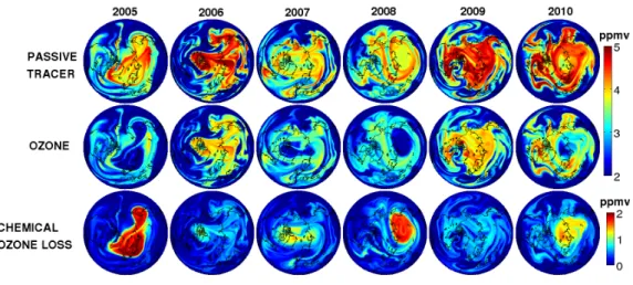
Fig. 3. Maps of passive tracer, ozone, and chemical ozone loss (passive tracer-ozone) calculated by Mimosa-Chim at 475 K on 15 March 2005–2010.
warm winters 2006 and 2009 show much smaller PSC area, limited in late-December/early-January with a peak value of about 0.8×10⁷km2. In winter 2007, the largest area of PSCs, 1.0×10⁷km2, is observed in late-December.
5 Results
We look into the details of ozone loss process of the recent winters in this section. Before starting the discussion on the loss, we first examine the ozone simulations. Since the pas-sive method used for the loss diagnosis depends on tracer simulations, the quality of the model simulations has to be checked against measurements. Therefore, we compare the ozone calculations with MLS observations, as the instrument provides measurements of a number of compounds linked to polar ozone loss since its launch in 2004. It is followed by a discussion of the ozone loss estimated from the simula-tions. The temporal evolution of vortex averaged ozone loss in Mimosa-Chim and MLS are diagnosed afterwards. The ozone loss features are interpreted using modelled and mea-sured chlorine activation in terms of ClO data. We later focus on the ozone loss analyses at two representative altitudes in the lower (475 K) and middle stratosphere (675 K).
5.1 Ozone: simulation and comparison with MLS
Figure 2 displays the vertical distribution of the Mimosa-Chim and MLS ozone together with their difference, sam-pled at the same time and location of the satellite observa-tions. The results are averaged inside the polar vortex de-fined as the area enclosed inside 65◦N of equivalent latitude (EqL) (see M¨uller et al., 2008 for further discussions on ade-quate definition of polar vortex). Due to early final warming (since there was no strong or well-defined polar vortex, we take the major warming in late-January/early-February 2006
and 2009 as the final warming), the data beyond the events are not considered in this study.
Both simulations and measurements show similar maxi-mum and exhibit a rather good agreement, with differences within ±0.5 ppmv depending on isentropic level and time. In general, the comparison yields good agreement in the lower stratosphere, below 500 K in particular. The calculations are in good agreement with the observations in the winters 2007, 2008 and 2009. The model captures well the ozone enhancement during the SSWs, specifically at higher alti-tudes, in January–February 2006 and 2009. The simulated middle stratospheric ozone levels during these periods are higher than those of other winters in accordance with the ob-servations. In February 2010, the higher ozone values due to meridional transport of ozone rich air masses from lower latitudes, associated with a major SSW, can also be seen in both data sets. Inter-annual variability in the evolution of ozone with altitude is apparent in the figure. For instance, the winter 2005 shows low ozone values in the lower strato-sphere up to 600 K. Further, the ozone maximum in the win-ter 2007 is comparatively smaller than that of other winwin-ters. Nevertheless, as displayed in the right panel of Fig. 2, the simulations systematically overestimate (up to 0.7 ppmv) the observations in early-December and March above 600 K in all winters, due to differences in subsidence. This differ-ence is found to be largest in March 2005, and in December and March 2010. In 2006, the model shows higher values of around 0.25 ppmv from December to February at 500– 800 K. On the other hand, the calculations underestimate (up to 0.5 ppmv) the measurements in January–February below 450 K and above 675 K in most winters. Among the winters the smallest differences are found in 2008 and the largest dif-ferences in 2010.
0.4 0.4 0.4 0.8 0.8 0.8 1.2 1.6
Mimosa−Chim Ozone Loss
400 600 800 0.4 0.4 0.4 0.8 0.8 1.2 1.2 Aura MLS Ozone Loss
2005 .4 0.4 400 600 800 0.4 0.4 2006 0.4 0.4 0.8 Potential Temperature (K) 400 600 800 0.4 0.4 0.4 0.8 0.8 1.2 2007 .4 0.4 0.8 1.2 400 600 800 0.4 0.4 0.8 0.8 1.2 2008 0.4 400 600 800 0.4 2009 0.4 0.8 −30 0 30 60 90 400 600 800 Day of year 0.4 0.8 1.2 1.6 2010 0 30 60 90 0 0.2 0.4 0.6 0.8 1 1.2 1.4 1.6 1.8 2 ppmv
Dec Jan Feb Mar Jan Feb Mar
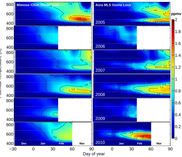
Fig. 4. Temporal evolution of the vertical distribution (350–850 K) of vortex averaged (≥65◦EqL) ozone loss (ppmv) estimated for the
Arctic winters 2005–2010. Left: the ozone loss derived from the difference between the passive tracer and the chemically integrated ozone by Mimosa-Chim. Right: the ozone loss derived from the difference between the Mimosa-Chim passive tracer and the ozone measured by MLS. The model fields are sampled at location of the MLS observations. Due to early vortex dissipation caused by the major warmings, the analysis does not extend beyond 10 February in 2006 and 2009. The ozone loss analysis in March 2010 are not included here because of very weak vortex and due to the tracer uncertainties after the major warming. Both data are smoothed for seven days. The white dotted lines represent the study altitudes 475 and 675 K.
5.2 Ozone loss
5.2.1 Simulations
The ozone chemical loss is computed from the difference be-tween a passive tracer initialised identically to ozone at the beginning of the simulation and the chemically integrated ozone (i.e., Ozone loss=Tracer-Ozone). As an example, Fig. 3 shows the passive tracer, ozone, and the difference (chemical ozone loss) calculated at 475 K on 15 March for each winter. In the figure, polar vortices with high ozone mixing ratios of around 4.5 ppmv corresponding to warm winters and reduced mixing ratios of around 3 ppmv corre-sponding to cold winters, are clearly shown.
Since the winter 2005 was one of the coldest, a vast vortex and large reduction in ozone is simulated, suggesting
sus-tained and high ozone depletion during the winter. Though not as large as observed in 2005, a significant area of low ozone levels off the pole is visible in 2008. Due to a strong SSW around mid-January, there was no vortex afterwards and hence high ozone is simulated in 2006 and 2009. In 2007, the vortex was seemingly smaller and therefore the ozone depletion is reduced. In 2010, even though there was a major SSW in late-January due to a planetary wave 1 event, the vortex split and merged again later. Therefore, a small dissipated vortex, displaced into the mid-latitude, with mod-erate ozone loss is simulated in that period. The maps dis-played in Fig. 3 clearly illustrate the strong inter-annual vari-ability in the meteorology and chemical ozone loss in the Arctic, with large losses (2 ppmv) diagnosed inside the polar vortex in 2005 and 2008, more limited loss in 2007 and 2010
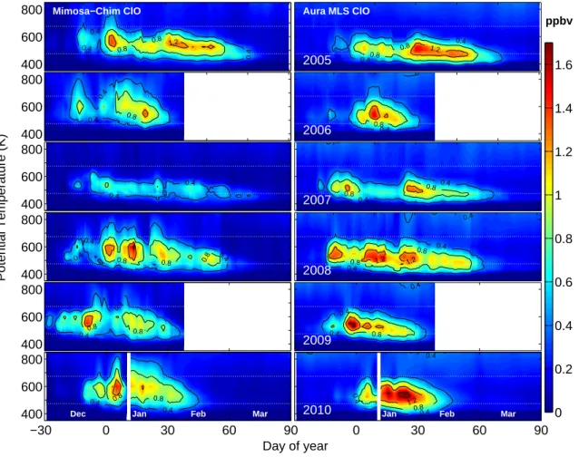
0.4 0.4 0.4 0.8 0.8 1.2 Mimosa−Chim ClO 400 600 800 0.4 0.4 0.4 0.8 0.8 1.2 Aura MLS ClO 2005 0.4 0.4 0.8 400 600 800 .4 0.4 0.8 2006 0.4 0.4 Potential Temperature (K) 400 600 800 0.4 0.4 0.4 0.8 0.8 2007 0.4 0.4 0.4 0.8 0.8 0.8 400 600 800 0.4 0.4 0.4 0.8 0.8 1.2 1.2 2008 0.4 0.40.8 0.8 400 600 800 0.4 0.4 0.4 0.8 2009 0.4 0.4 0.8 0.8 −30 0 30 60 90 400 600 800 Day of year 0.4 0.4 0.4 0.8 1.2 2010 0 30 60 90 0 0.2 0.4 0.6 0.8 1 1.2 1.4 1.6 ppbv
Jan Feb Mar
Dec Jan Feb Mar
Fig. 5. Temporal evolution of the vertical distribution (350–850 K) of vortex averaged (≥65◦EqL) ClO (ppbv) for the Arctic winters 2005–
2010. Left: Mimosa-Chim calculations and Right: MLS measurements. The Model and MLS ClO coincident profiles are selected for solar
zenith angles <89◦and local time between 10 h and 16 h. Both data are smoothed for three days. MLS ClO values are corrected for the
negative bias identified by Santee et al. (2008).
(0.8–1 ppmv), and the absence of vortex, as of 15 March, in 2006 and 2009. Thus, as discussed in Sect. 1, the most recent Arctic winters show a wide variety of polar processing, quite in line with previous northern winters.
5.2.2 Comparison with MLS: vertical features
Figure 4 (left panel) displays the vertical structure of the ac-cumulated chemical ozone loss computed from the simula-tions for the winters 2005–2010. The vortex averaged ozone loss computed from the model grids and at the MLS sam-pling points show rather small differences. Therefore, we present the ozone loss computed at the MLS footprints in-side the vortex for each winter for comparison purpose.
Among the winters, 2005 exhibits the largest ozone loss with a maximum of 1.7 ppmv in March around 475 K. The loss is spread vertically between 450 and 850 K in January– February, reaching 1.5 ppmv above 600 K in late-February. In March, most of the loss is confined between 400 and
600 K. Comparatively large losses are also found in the cold winters 2007 and 2008. In 2007, the ozone loss shows a double peak feature with a maximum of 1.3 ppmv at 675 K. In 2008, the ozone loss is delimited between 450 and 600 K with a peak loss of 1.4 ppmv around 475 K. Little loss is com-puted above the 650 K level in this winter. Due to major warmings, the winters 2006 and 2009 show limited ozone loss, not exceeding 0.8 ppmv. The winter 2009 presents the smallest vertical extent in the diagnosed ozone loss, which is mainly centred below 650 K until the final warming. In 2010, a wide spread loss of around 0.9 ppmv from mid-January to February at 450–800 K with a peak loss of about 1.1 ppmv at 600 K is estimated. Ozone loss analysis for this winter is restricted until February due to problems in tracer descent after the warming, as identified from the modelled N2O
iso-pleths. Additionally, there was no activated chlorine to in-duce a sustained loss afterwards in March. Study by Goutail et al. (2010) also show that the ozone loss has stopped by the end of February.
Figure 4 (right panel) describes the temporal evolution of the vertical distribution of vortex averaged ozone loss de-rived from the observations. Ozone loss from the measure-ments is computed in a similar way as for the simulation (the difference between the passive ozone tracer sampled at each measurement point and observed ozone). In agreement with the calculations, comparatively large losses are estimated from the measurements in 2005 and 2008, reaching 1.5 and 1.4 ppmv respectively. The simulations reproduce quite well the gross features of observed ozone loss in each winter, e.g. its onset in the course of the winter, the altitude of its maxi-mum and its vertical distribution. The agreement between the model and MLS is particularly good in 2006, 2007, 2008 and 2009, where the differences are mostly within ±0.2 ppmv. As shown in Fig. 2, the modelled ozone in March is com-paratively higher and therefore, the maximum ozone loss is slightly lower in the model depending on altitude. In 2010, the computed loss from MLS is about 0.5 ppmv larger than that of Mimosa-Chim. This difference is due to relatively higher values (0.5–0.8 ppmv) in simulated ozone throughout the winter at 500–700 K and also because of larger passive tracer values calculated after the warming, as compared to previous winters. However, in 2005 the model does simulate the second ozone loss maximum observed around 600 K, al-beit with a lesser amplitude. In both cases, the results show a large ozone loss in the middle stratosphere, as compared to other winters followed by its strong decrease in March. In addition, both the simulations and observations provide the highest ozone loss above 500 K in 2007. To further investi-gate the causes of differences in the estimated ozone loss, we analyse the measured chlorine activation and its representa-tion in the model in the next secrepresenta-tion.
5.2.3 Comparison: ClO and Chlorine activation
Figure 5 compares the temporal evolution of vertical dis-tribution of vortex averaged ClO extracted from MLS ob-servations and Mimosa-Chim simulations for various win-ters. As expected from large areas of PSCs, the observa-tions show high chlorine activation in 2005, 2008, and 2010 with enhanced ClO values in the lower stratosphere up to about 600 K. In these winters, vortex averaged ClO reach 1.2–1.5 ppbv around 550 K in January. Chlorine activation usually starts in December above 475 K (in late-December during the first two winters and a little earlier in the later ones) and then extends lower down in the course of the win-ter. Both simulated and measured ClO occupy a larger verti-cal stretch and exhibit higher values in January 2010 as com-pared to other winters, consistent with higher ozone loss es-timated in that period. The simulations generally reproduce the observed ClO and its variability throughout the winter quite well, although some differences are seen. In 2005 and 2010, a stronger chlorine activation extending up to 650 K is simulated in late-December as compared to the observa-tions. In 2005, later during the winter, higher ClO values
are observed in MLS extending up to mid-March. This dis-crepancy explains the stronger ozone loss derived from the observations at 500–600 K in March (see Fig. 4). In 2007, Mimosa-Chim clearly underestimates the observed chlorine activation. The vortex averaged ClO in Mimosa-Chim is lower by about 0.4 ppbv, which explains the underestimation of ozone loss in the simulations for that year. In other win-ters, the simulations show generally a good agreement with the observations at most altitudes. A closer examination of the ozone loss in the lower and middle stratosphere at two representative isentropic levels, 475 and 675 K, is presented in the following sections.
5.2.4 Comparison: lower stratosphere
As shown by Fig. 4, the simulated ozone loss until January is generally within 0.2 ppmv and it varies in January–March for each year at 475 K. The maximum ozone loss derived from the simulations is, respectively, 1.7, 0.7, 1.1, 1.3, 0.9 and 0.9 ppmv in 2005, 2006, 2007, 2008, 2009 and 2010. The corresponding observed losses are in turn 1.5, 0.7, 1.2, 1.4, 0.8 and 0.9 ppmv, and are in very good agreement with the simulated ones, with differences within ±0.2 ppmv.
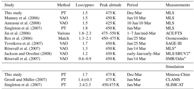
The ozone loss obtained from our study is in general good agreement with that obtained from other techniques for the winter 2005 (WMO, 2007), 2006 (Manney et al., 2007) and 2007 (R¨osevall et al., 2008). Table 1 presents the compar-ison of ozone loss derived from various measurements and model calculations for the winter 2005. The maximum loss simulated at 475 K is about 1.7 ppmv (1.5 ppmv from MLS) in 2005, which compares well with that of Grooß and M¨uller (2007). Our loss estimations are also in very good agreement with those of Jackson and Orsolini (2008); R¨osevall et al. (2007); Singleton et al. (2007) and Tsvetkova et al. (2007), as we estimate comparable values in respective periods. It must be noted that the ozone loss computed from MLS observa-tions by Manney et al. (2006) and Amraoui et al. (2008) also show the same maximum of 1.5 ppmv, which greatly support our ozone loss computation technique. However, the peak ozone loss altitude shown by some works are generally about 25 K lower than in our analysis. Such a discrepancy among various techniques was also noted by Grooß et al. (2005a) for the winter 2003. The only diagnosis that departs consid-erably from all other evaluation is R¨osevall et al. (2007), with Submillimeter Radiometer (SMR) data. This could be due to the peculiarity of their method, which is prone to more mix-ing and dilution in the vortex air. The vertical motion was not represented explicitly but was calculated from N2O
measure-ments for their analyses. Other details regarding the method can be found from Jackson and Orsolini (2008), who pro-vide a brief comparison of most ozone loss estimation tech-niques. In agreement with the measured and simulated ozone loss and Apsc, the chlorine activation is predominant in 2005 and 2008, moderate in 2010, and weak in 2007 at 475 K. The winters 2006 and 2009 started off with low temperatures
Table 1. The vortex averaged (≥65◦EqL) ozone loss estimated in volume mixing ratio (ppmv) from Mimosa-Chim and MLS data, compared to different studies for the Arctic winter 2005. The initial offset in tracer and Mimosa-Chim ozone is corrected with respect to MLS ozone to avoid any bias in ozone loss computations. The passive tracer method is denoted by PT and the vortex averaged/profile descent method is
denoted by VAO. The ozone loss analyses based on assimilated data are indicated by∗.
Study Method Loss/ppmv Peak altitude Period Measurements
This study PT 1.5 475 K Dec/Mar MLS
Manney et al. (2006) VAO 1.5 450 K Jan/10 Mar MLS
Amraoui et al. (2008) VAO 1.5 425 K 10 Jan/10 Mar MLS
Singleton et al. (2007) PT 1.8 450 K Jan/Mar MLS
Jin et al. (2006) Various 1.8–2.3 475–550 K 1–7 Jan/mid-Mar ACE/FTS
Rex et al. (2006) Match 1.3–2.1 450–475 K Jan/25 Mar Ozonesondes
Tsvetkova et al. (2007) VAO 1.7 450 K Jan/25 Mar SAGE III
R¨osevall et al. (2007) VAO 1.3 450 K Jan/14 Mar MLS∗
Jackson and Orsolini (2008) VAO 1.2 450 K early-Jan/early-Mar MLS/SBUV2∗
R¨osevall et al. (2007) VAO 0.6–0.9 450 K Jan/14 Mar SMR/Odin∗
Simulation
This study PT 1.7 475 K Dec/Mar Mimosa-Chim
Grooß and M¨uller (2007) PT 1.4±0.3 475 K Jan/Mar CLAMS
Singleton et al. (2007) PT 2.4/2.3 450/475 K Jan/Mar SLIMCAT
and therefore, were subjected to early chlorine activation and ozone loss as compared to other winters. It has to be re-called that a similar range of ozone loss values, from 0.7 to 2.3 ppmv, was also computed for the cold Arctic winter 2000 by various methods (Newman et al., 2002).
5.2.5 Comparison: middle stratosphere
As evident in Fig. 4, the simulated ozone loss at 675 K is around 0.2 ppmv in early-January in most winters. The max-imum loss reaches 1.1, 0.7, 1.2, 0.8, 0.3, and 0.9 ppmv in 2005, 2006, 2007, 2008, 2009, and 2010, respectively. The loss derived from observations show successively 1.2, 0.6, 0.8, 0.7, 0.5, and 0.7 ppmv for the corresponding winters. The simulated ozone depletion shows good agreement with that of observations, within ±0.2 ppmv. The large loss cal-culated around 675 K in January–February 2005 is also con-firmed by other estimations (Jin et al., 2006; Rex et al., 2006; Grooß and M¨uller, 2007; Tsvetkova et al., 2007; Jackson and Orsolini, 2008). The high ozone depletion simulated at 675 K is in good agreement with that of Grooß and M¨uller (2007), who estimate a similar loss at this altitude. This double peak structure is not pronounced in the analysis of Singleton et al. (2007) and thus, the measured and simulated ozone loss in their study are considerably smaller (about 0.7 ppmv) than our estimates. There is only a little amount of active chlorine present at 675 K, as most of it is found below 600 K. There-fore, key factors driving ozone loss at 675 K will be discussed in the succeeding sections.
6 Discussion
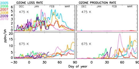
6.1 Ozone loss and production rates
To gain further insights into the inter-annual variability of ozone in the Arctic vortex, we have calculated the ozone loss and production rates for the winters 2005–2010. The fol-lowing equation was applied to compute the vortex averaged ozone loss and production rates from the model output.
δO3(θ,j ) (ppbv/sh) = λeq=90 X λeq=65 δO3(θ,j,λeq) ×sh(θ,j,λeq) λeq=90 X λeq=65 sh(θ,j,λeq)
where, δO3(θ,j )is the ozone loss or production averaged
within EqL (λeq) ≥65◦for each model isentrope (θ ) and day
(j ). δO3(θ,j,λeq) is the instantaneous ozone loss or
produc-tion calculated by the model for each grid point defined by latitude (φ) and longitude (ψ ) for each θ and j . sh(θ,j,λeq)
is the sunlit hour calculated with respect to solar zenith angle
<95◦that varies between 0 and 1 for complete darkness to full illumination. The λeqis computed for each model grid
(θ ,φ,ψ) and for each day using potential vorticity (PV) data. Figure 6 shows the vortex averaged instantaneous ozone loss and production rates in ppbv per sunlit hour (ppbv/sh) at 475 (top panel) and 675 K (bottom panel).
Fig. 6. Vortex averaged (≥65◦EqL) chemical ozone loss and production rates at 475 and 675 K, expressed in ppbv per sunlit hour (ppbv/sh), for the Arctic winters 2005–2010. The data are exempted from temporal smoothing to explicitly show the effect of daily movement of vortex and its impact on ozone production and loss rates.
6.1.1 Lower stratosphere
At 475 K, the winter 2005 shows the largest loss rate of around 5 ppbv/sh in February. In 2010, loss rates of 3– 5 ppbv/sh are calculated in mid-January/mid-February, while relatively lower depletion rates are found in 2008 and 2007 during these months. The warm winters 2009 and 2006 show loss rates up to 3–4 ppbv/sh in December and mid-January respectively, which are higher than those of the cold winters during the same period. There is hardly any ozone produc-tion at this isentropic level.
For the winters discussed here, there are no other stud-ies with which to compare our simulated ozone loss rates. Therefore, we compare the results of previous Arctic win-ters from Frieler et al. (2006). They derive ozone loss rates (seven/ten day averages) of 5–10 ppbv/sh at 490 K in 1995, 5–8 ppbv/sh at 475 K in 1996, 6–7 ppbv/sh at 500 K in 2000, 4.5–8.5 ppbv/sh at 475 K in 2001 and 4–5 ppbv/sh at 475 K in 2003 in January. Since calculation of Frieler et al. (2006) is based on a box model, the figures are not directly compa-rable. However, our results are generally in good agreement with their analyses. For instance, (i) both observations and our simulations show higher loss rates in late-January/early-February, (ii) the loss rates in warm winters rarely extend beyond January, but are higher than those for most cold win-ters for the same period, and (iii) cold winwin-ters with sustained loss show higher simulated loss rates in January/mid-March, consistent with the measured rates.
6.1.2 Middle stratosphere
At 675 K, ozone loss and production rates tend to increase with time until February. The largest loss rates of our study are found in February–March 2008, around 12 ppbv/sh. In
2010, elevated loss rates of 4–9 ppbv/sh are simulated in mid-February/mid-March. A similar evolution of production rates is also calculated during these two winters, in which the lat-ter shows a massive production of 5–19 ppbv/sh. The large loss of 2–6 ppbv/sh is masked by enhanced production of 2–14 ppbv/sh in mid-March 2005. The loss rates dominate over production rates in 2007 except in late-February, which is consistent with the highest ozone loss found at 675 K in March. The warm winter 2006 records the largest loss and production rates in December–January in line with the high chlorine activation and ozone loss during the period.
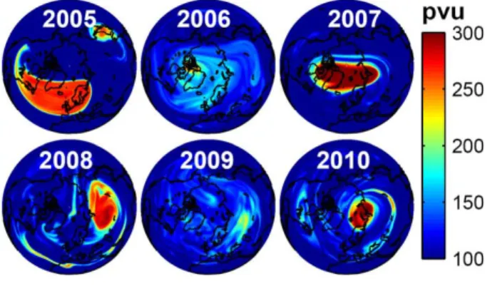
Figure 7 shows the PV maps on 15 March of each year at 675 K. Since ozone production depends solely on sunlight, the movement of vortex over illuminated regions causes its variation. As can be seen from the figure, the displacement of the vortex to the mid-latitudes explains the reasons for higher production rates in 2005, 2008 and 2010 as compared to other winters. This is also clearly seen in late-January/early-February in 2006 and 2009, and late-late-January/early-February/early-March 2010, during which the polar vortices were displaced off the pole by major SSW events (Manney et al., 2006; Flury et al., 2009; Kuttippurath et al., 2010). Further, it is evident from Fig. 6 that the production rate in March increases with time, which is well anticipated as the final warming approaches. On the other hand, a pole centred vortex and hence, compar-atively diminished production rates are found in 2007.
6.2 Ozone loss and chemical cycles
In order to better understand the prime chemical cycles driv-ing the ozone loss inside the vortex in the lower and mid-dle stratosphere, we have evaluated contribution of various chemical cycles as a function of time at 475 and 675 K for the winters discussed here. Contribution of each cycle is given in
9924 J. Kuttippurath et al.: Arctic ozone loss variability and chemical cycles
Fig. 7. Maps of potential vorticity (1 PV units
(pvu))=10−6km2kg−1s−1) calculated from ECMWF data
on 15 March 2005–2010 at 675 K. The maps also display the strength and position of polar vortex on 15 March in each winter.
percent of the total contribution from all cycles. This contri-bution is shown in Fig. 8 left panel for the lower stratosphere (475 K) and right panel for the middle stratosphere (675 K).
6.2.1 Lower stratosphere
The importance of halogen cycles in ozone destroying pro-cess in the polar lower stratosphere is relatively well known (e.g. WMO, 2007) and this study too finds similar results. At 475 K, the ClO–ClO and ClO–BrO cycles represent 80–90% of the total loss (e.g. Frieler et al., 2006; Woyke et al., 1999). The ClO–O cycle contributes 10% to the loss throughout the winter at this level, consistent with a previous study at 465 K based on UARS MLS (Upper Atmosphere Research Satel-lite MLS) measurements in the Arctic and Antarctic winter of 1993 (MacKenzie et al., 1996). The ClO dimer cycle is prominent in January/mid-March (since the ozone loss be-fore January is very small, the contribution bebe-fore the pe-riod is not shown), with a maximum contribution of ∼50% in mid-January/mid-February. Because of its quadratic depen-dence on ClO, the efficiency of the ClO–ClO cycle to destroy ozone falls very rapidly when active chlorine returns to reser-voir forms at the end of the winter. This is not the case for the contribution of BrO–ClO, which decreases not as rapidly in these conditions, and therefore becomes larger than that of the ClO–ClO cycle in early-March. When the ClO dimer cy-cle becomes less important, the contribution from ClO–BrO enhances. A similar result was also observed by Butz et al. (2007) in the Arctic winter 1999 from balloon-borne mea-surements. From early-March onwards, as there are no PSCs and chlorine activation the contribution of the HOxand NOx
cycles grow quickly and become the active ozone depleting cycles in the second half of the month.
Another interesting feature to note is the contribution of the cycles in 2010. During this winter temperatures were rel-atively high and as emphasised previously, the vortex was
subjected to a major SSW and subsequent split. Therefore, in early-February the ClO–ClO contribution fell dramatically and contribution from other cycles (HOxand BrO–ClO
cy-cles in particular) dominated later during the winter for the reasons stated above. Contribution from HOx dominates
during warming periods, and is demonstrated by its rela-tively higher contribution in the vortex dissipation (mid/late-March) or major SSW periods (late-January 2006 and 2009, and mid-February 2010). Since increase in mixing ratios of H2O and HNO3 during warmings are expected (e.g. Flury
et al., 2009) and are the sources of HOx, contribution from
this cycle outweighs others (e.g. Marchand et al., 2005). The maximum contribution of the ClO–ClO cycle to the total loss varies from ∼50% in cold winters to ∼40% in warm winters. In contrast, contribution from ClO–BrO equals that of ClO–ClO in warm winters and decreases to
∼25–30% in cold winters. The larger difference in the contribution of both cycles, during the period of sustained ozone loss, is found in the winter 2008 from January to late-February.
Our results on the contribution of halogens to the total loss are consistent with those found in Frieler et al. (2006). Using a photochemical box model, they also show a contribution of 50% from the ClO dimer, ∼27–48% from BrO–ClO and 5– 10% from ClO–O to the total loss in the Arctic winters 1995, 1996, 2000, and 2001, and in the Antarctic winter 2003 in the lower stratosphere. They also find that the efficiency of the BrO–ClO cycle increases with faster photolysis rate of ClO dimer. Studies using UARS MLS measurements for the Antarctic winters 1992–1994 also point out that these two cycles account nearly for 90% of the total loss in the lower stratosphere (Wu and Dessler, 2001). Therefore, our study confirms the fact that the odd oxygen loss in the polar winter lower stratosphere is dominated by the ClO dimer and ClO– BrO catalytic cycles, which is quite in line with our current theoretical understanding and is consistent with the findings of previous studies.
6.2.2 Middle stratosphere
In contrast to what is found at 475 K, the halogen catalysed cycles play comparatively a small role in the Arctic ozone depletion at 675 K, as demonstrated in Fig. 8 (right panel). At this level, the ozone loss is essentially due to the NO– NO2 cycle, which represents 50–75% of the total depletion
in February–March, complemented by the ClO–O cycle that contributes about 10–20% to the total loss during the period. The ClO–O contribution is found to be as large as 20–55% in January. However, ozone loss at this altitude during the period is very small (0–0.3 ppmv). The contribution of HOx
cycle, which is about 10–20% in January, increases during the course of the winter to become equal or larger than that of ClO–O in late winter. The rate limiting step in all these cycles is the combination of the oxygen atom with a specific molecule (for e.g. HO2+O for HOx, and ClO+O for ClOx).
Fig. 8. Vortex averaged (≥65◦EqL) relative contribution of selected ozone depleting chemical cycles to the total chemical ozone loss at 475 (left panel) and 675 K (right panel) in the Arctic winters 2005–2010. The data are smoothed for ten-days. The dotted lines represent 50% and the top lines of each plot represent 100% contribution.
Therefore, the availability of O-atoms mainly determines the efficiency and duration of these cycles and thus, the accumu-lated ozone loss at 675 K.
The inter-annual variability is relatively strong for ClO–O and NO–NO2cycles, markedly in January. The variability of
ClO–O contribution is linked to the formation of PSCs. The NO–NO2cycle contributes 10–20% in 2010, 2009, 2008 and
2006, but 30–45% in 2005 and 2007 in January. The maxi-mum ozone depletion simulated around 675 K in 2007 is in agreement with the relatively high contribution of NO–NO2
during the winter. However, similar contribution of this cycle in other winters is compensated by large ozone production, as discussed in Sect. 6.1.
Unlike for lower stratosphere, only a few studies are per-formed on the aspects of contribution of different chemical
cycles to the total loss above 650 K. Moreover, the available studies on previous winters address contribution of the cy-cles in some specific issues such as ozone loss due to addi-tional NOx loading during solar proton events or warming
events (Grooß et al., 2005a; Vogel et al., 2008). For instance, box model calculations by Konopka et al. (2007) noted the efficiency of NOx, HOx, ClO–ClO and BrO–ClO cycles as
76, 12.5, 3.5 and 1% respectively at 600–900 K during the warm Arctic winter 2003. Interestingly, large loss of ozone at higher altitudes with a double peak structure (as found in 2005) was simulated in this winter too (Grooß et al., 2005a). Simulated ozone loss for the winter is comparable to that of 2005, with a maximum of around 1.4 ppmv at 475 and 675 K. They also linked the higher loss above 600 K to the exposure of vortex air to sunlight that began early during this
dynamically disturbed winter, in tune with their analyses for the southern winter 2002 (Grooß et al., 2005b). These results are in agreement with our analysis for the warm winters, dur-ing which the contribution from NOx is larger than that of
the cold winters, inducing higher ozone loss above 600 K. Therefore, in PSC-free polar stratosphere in 600–850 K, the NO–NO2cycle plays a major role in ozone depletion.
6.3 Partial column ozone loss
To complement our ozone depletion analysis based on mix-ing ratio, we have computed the ozone column loss for each winter from both the Mimosa-Chim simulations and MLS observations. For the integration, the model ozone and tracer profiles were interpolated to the MLS sampling points inside the vortex (≥65◦EqL). The MLS profiles were then interpo-lated to the vertical levels of the model in order to have the same column computation procedure for both data sets. Most studies concentrate the ozone column loss in the lower strato-sphere, and therefore we have calculated the loss in the 350– 550 K column range. In order to analyse the contribution from middle stratosphere by cycles like NOx, as discussed
in the previous section, we have computed the column loss for the whole 350–850 K range. Except for the warm win-ters 2006, 2009 and 2010, the accumulated column loss are estimated from December through the end of March. Calcu-lations for the warm winters are restricted to 10 February for 2006 and 2009, and 28 February for 2010, consistent with our previous analysis. The daily average ozone and tracer data are used for these column loss calculations. The re-sulting column losses in 350–550 K and 350–850 K for each winter are given in Table 2.
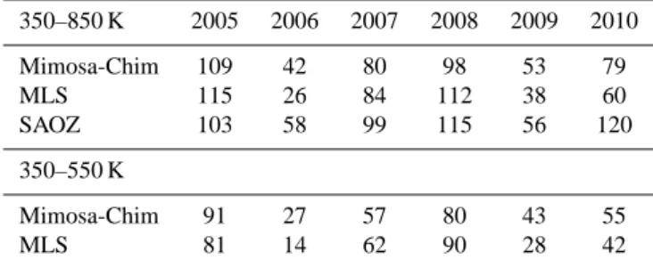
For the 350–850 K partial column, the largest loss is found in 2005 and the lowest loss in 2006, in agreement with our previous discussion on the vertical distribution of ozone loss. In 2005 and 2008, the column loss simulated by the model is respectively 109 and 98 DU while that derived from the MLS observations amounts to respectively 112 and 115 DU. In the warm winters 2006 and 2009, a limited loss reaching 53 DU (in 2009) is simulated. The most recent warm win-ter 2010 is characwin-terised by a moderate loss of 79 DU by the end of February. The column loss calculated by the model overestimates the measured loss in all three warm winters (2006, 2009 and 2010) by 16–19 DU. These figures from Mimosa-Chim and MLS compare reasonably well with those derived from the ground-based total column observations from UV-visible SAOZ (Systeme d’Analyse par Observation Zenithale) network in the Arctic (Goutail et al., 2005, 2010). As shown by the simulations, large loss in cold and relatively small loss in warm winters are computed from the SAOZ measurements. The SAOZ estimations are generally in good agreement with those of Mimosa-Chim/MLS, with devia-tions within 20 DU. In 2010, the difference is much larger, reaching 40 and 60 DU with the simulations and MLS obser-vations respectively. The offset between SAOZ and
Mimosa-Table 2. The vortex averaged (≥65◦EqL) accumulated ozone
par-tial column loss (DU) estimated in 350–850 and 350–550 K from the MLS sampling inside the vortex and corresponding Mimosa-Chim simulations interpolated to the observed points for each win-ter (121 Days from December to March). The SAOZ total column loss computations for the winters are compared to Mimosa-Chim and MLS loss estimates in 350–850 K. The calculations for the warm winters 2006 and 2009 are performed for 72 days (from 1 December to 10 February), and 2010 for 90 days (from 1 December to end of February). The maximum loss is found (shown below) around 23–25 March in cold winters. The initial offset between tracer and MLS/Mimosa-Chim ozone is corrected with respect to MLS ozone to account for any biases in ozone loss computations. The column loss is computed from the the daily average of ozone and tracer column found inside the vortex.
350–850 K 2005 2006 2007 2008 2009 2010 Mimosa-Chim 109 42 80 98 53 79 MLS 115 26 84 112 38 60 SAOZ 103 58 99 115 56 120 350–550 K Mimosa-Chim 91 27 57 80 43 55 MLS 81 14 62 90 28 42
Chim/MLS ozone loss can be due to differences in the vortex limit criteria and sampling. That is, the ground-based estima-tions depend on seven staestima-tions in the vortex, while the MLS sampling covers relatively quite well the polar region. Ad-ditionally, the ground-based analysis uses slightly different vortex criterion and the column measurements do not sample vortex air at all altitudes, whereas only vortex air is consid-ered in our analysis.
The ozone loss in the lower stratosphere, in 350–550 K, shows similar features as noted in the 350–850 K column range. Namely, (i) cold and warm winters exhibit respec-tively higher and lower ozone column depletion, (ii) the ozone loss estimated from MLS is larger than that from the model alone (except in 2005 in 350–550 K), and (iii) the modelled loss is larger by about 10–20 DU than the measured depletion in warm winters.
In a study using Match ozonesonde measurements in the Arctic, Harris et al. (2010) derive an accumulated ozone col-umn depletion of 72 DU in 2007 and 65 DU in 2008 in 380– 550 K. Both Mimosa-Chim and MLS loss estimations under-estimate the Match results in 2007 by 10–15 DU and overes-timate them in 2008 by 15–25 DU. In contrast to the Match results, our estimations provide comparatively larger ozone loss in the cold winter 2008. The simulated loss in 2006 is in good agreement with that of Feng et al. (2007), who cal-culate a loss of about 32 DU in early-February in 380–550 K. The comparison of ozone column loss estimates for the Arc-tic winter 2005 is presented in a separate section as there are several published results available for a discussion.
Table 3. The vortex averaged (≥65◦EqL) ozone partial column loss (DU) computed from Mimosa-Chim and MLS data in 350–550 K and 350–675 K are compared to various results for the Arctic winter 2005. Individual vortex definition is used by each study. The error estimation provided by the respective studies are given together with the ozone loss values. Here, the column title “Period” represents the time line of individual studies and “Max. Loss” indicates the day on which the maximum ozone depletion is estimated. The column length used for the ozone loss computations are relatively small for the estimates given in italics.
Study Data Column Period Max. Loss Loss (DU)
This study MLS 350–675 K December–March March end 109
– MLS 350–550 K December–March March end 81
Singleton et al. (2007) Satellites 400–550 K January/March March end 90±15
Tsvetkova et al. (2007) SAGE III 350–625 K January/25 March 25 March 116±10
Jin et al. (2006) ACE-FTS 375–650 K 1–7 January/mid-March 15 March 116
Rex et al. (2006) Match 350–550 K January/25 March 25 March 127±21
von Hobe et al. (2006) in-situ 344–460 K 7 March 7 March 62−+178
Simulations
This study Mimosa-Chim 350–675 K December–March March end 107
– Mimosa-Chim 350–550 K December–March March end 91
Grooß and M¨uller (2007) CLAMS 380–580 K January–March 23 March 69±20
Feng et al. (2007) SLIMCAT 380–550 K December–March March end ∼140
The difference between the partial column loss estimated in 350–550 K and 350–850 K (i.e., 1 Loss=Loss350−850K–
Loss350−550K) averaged over the studied winters is equal
to 18.0±5.2 and 19.7±8.6 DU for the MLS observations and Mimosa-Chim simulations respectively. Such a differ-ence, mainly due to the effect of NOxchemistry in the
mid-dle stratosphere, has to be taken into account when com-paring polar ozone loss computed from total ozone ob-servations with that derived from ozone profile measure-ments/simulations.
6.3.1 Partial column loss in 2005
Since the winter 2005 was one of the coldest in the decade, a number of ozone loss estimations based on measurements and simulations have been published. Table 3 compiles the vortex averaged ozone column loss calculated from various data sets. For a better comparison with other results we have also estimated the loss in 350–675 K from both Mimosa-Chim simulations and MLS observations. As shown by the table the loss estimated by different studies generate differ-ent results. The Mimosa-Chim analysis shows a good agree-ment with Singleton et al. (2007), who also compute a sim-ilar loss from MLS observations. The Mimosa-Chim/MLS ozone loss in 350–675 K show a good agreement with those from Jin et al. (2006) and Tsvetkova et al. (2007). The larger loss simulated in Feng et al. (2007) is due to the higher vor-tex descent and accompanied increase in chlorine loading in the lower stratosphere of their model. The ozone loss com-putation from von Hobe et al. (2006) shows the lowest value among these analyses while that of Rex et al. (2006) pro-vides the largest estimate. The accumulated loss in von Hobe et al. (2006) was estimated on 7 March, which is much
ear-lier than in other studies (around 25 March) and there was a strong vortex and sustained loss afterwards. Also, the loss was estimated only up to 460 K, which is much lower than the column upper limit considered in other studies. Such a discrepancy in the altitude range used for the analyses is one of the reasons for the spread in the results. Another possi-ble reason for the difference is that most works use their own vortex criterion for the ozone column loss estimation.
Regarding the ozone loss derived from various model re-sults, the simulations by Grooß and M¨uller (2007) provide the lowest estimate. This offset can be due to a different sampling of the vortex by the model grid, as compared to the satellite observations. In order to check this, we aver-aged the simulated loss over all the model grid points (not only at the footprint of MLS observations) using the same vortex criterion of Grooß and M¨uller (2007) and obtained a loss of 73 DU in 350–550 K (our model vertical levels are different). This estimate is in very good agreement with the calculation of Grooß and M¨uller (2007). Another important fact to note is the sampling of the vortex by the MLS sensor, which is limited to 82◦. In contrast, the model grid spans to the full 90◦including the pole. Therefore, the average cal-culated from the models can cover the area inside the vortex from this additional latitude region of 8◦(i.e., 83–90◦N) too, and hence, this average can differ from the mean loss esti-mated at the satellite footprints. In short, the differences in vortex sampling, altitude range, time period and vortex def-inition of the analyses have to be taken into account when comparing different ozone loss estimations.
7 Conclusions
The evaluation of vortex averaged ozone loss from the model and satellite observations shows large variability in the Arctic winters 2005–2010, in accordance with analyses performed for previous northern winters. The cold winters 2005 and 2008 record the highest loss with peak ozone loss around 475 K. In 2007, the maximum loss is estimated at a higher al-titude, around 650 K and the minimal loss among the winters is obtained in the warm winters 2006 and 2009. At 475 K, the cumulative ozone loss ranges from 0.7 ppmv in 2006 to 1.5–1.7 ppmv in 2005. At 675 K the loss ranges from 0.3– 0.5 ppmv in 2009 to 1.3 ppmv in 2005. In general, the ozone loss values derived from the Mimosa-Chim simulations and MLS observations, combined with the model passive tracer, are in good agreement and the differences are mostly within the estimated accuracy of the observations.
It has to be noted that, since there is a large variability in peak ozone loss altitude from one year to the next, analysis or comparison of ozone loss at specific altitudes is neither com-plete nor well-represented as far as the variability of Arctic winters is concerned. Therefore, care has to be taken while interpreting the ozone loss estimated at specific altitudes, to characterise or compare different winters.
Model runs with specific chemical cycles suggest that the halogen cycles; ClO–ClO contributes ∼40–50% and BrO– ClO contributes ∼30–40% to the total loss in December-February at 475 K. These cycles depend on temperatures in the lower stratosphere, PSCs, heterogeneous reactions on PSCs and thus the Arctic meteorology. The NO–NO2cycle
is the key mechanism that depletes about 60–75% of ozone in the middle stratosphere, which is essentially predominant in January–March period. In warm winters, the contribution from HOx cycle gradually increases and eventually
domi-nates in the lower stratospheric ozone loss process after the major warming.
The ozone partial column loss estimated in 350–850 K from Mimosa-Chim calculations at the MLS footprints in-side the vortex shows about 109, 42, 80, 98, 53, and 79 DU in 2005, 2006, 2007, 2008, 2009 and 2010, respectively, and are in good agreement with those of the MLS and SAOZ ob-servations within the limits of their error estimations. There is a significant difference (∼19±7 DU) in the ozone column loss estimated between the ranges 350–850 and 350–550 K. The additional loss above 550 K is mainly due to NOx
chem-ical cycles and should be accounted for while estimating the column loss from ozone profile measurements/simulations. This is particularly important in cold winters with vertically spread ozone depletion (e.g. in 2005) and warm winters with peak ozone loss above 550 K (e.g. in 2009).
Acknowledgements. The authors would like to thank Cathy Boonne of IPSL/CNRS Paris for the REPROBUS data. They also thank Andrea Pazmino and Julien Gazeaux of CNRS/LATMOS Guyan-court/Paris for their co-operation during this study. They extend their gratitude to the reviewers, Jens-Uwe Grooß and Mar-tin Dameris (the Editor) for their constructive comments on the article that helped to further improve the quality of this article. The MLS data used in this study were acquired as part of the NASA’s Earth-Sun System Division and archived and distributed by the Goddard Earth Sciences (GES) Data and Information Services Center (DISC). The work is supported by funds from the
ANR/ORACLE–O3France and the EU SCOUT–O3projects.
Edited by: M. Dameris
The publication of this article is financed by CNRS-INSU.
References
Amraoui, L. El, Semane, N., Peuch, V.-H., and Santee, M. L.: In-vestigation of dynamical processes in the polar stratospheric vor-tex during the unusually cold winter 2004/2005, Geophys. Res. Lett., 35, L03803, doi:10.1029/2007GL031251, 2008.
Burkholder, J. B., Orlando, J. J., and Howard, C. J.: Ultraviolet
absorption cross-sections of Cl2O2between 210 and 410 nm, J.
Phys. Chem., 94, 687–695, 1990.
Butz, A., B¨osch, H., Camy-Peyret, C., Dorf, M., Engel, A., Payan, S., and Pfeilsticker, K.: Observational constraints on the ki-netics of the ClO-BrO and ClO-ClO ozone loss cycles in the Arctic winter stratosphere, Geophys. Res. Lett., 34, L05801, doi:10.1029/2006GL028718, 2007.
Davies, S., Chipperfield, M. P., Carslaw, K. S., et al.: Mod-elling the effect of denitrification on Arctic ozone deple-tion during winter 1999/2000, J. Geophys. Res., 107, 8322, doi:10.1029/2001JD000445, 2002.
Feng, W., Chipperfield, M. P., Davies, S., von der Gathen, P., Kyr¨o, E., Volk, C. M., Ulanovsky, A., and Belyaev, G.: Large chemi-cal ozone loss in 2004/2005 Arctic winter/spring, Geophys. Res. Lett., 34, L09803, doi:10.1029/2006GL029098, 2007.
Flury, T., Hocke, K., Haefele, A., K¨ampfer, N., and Lehmann, R.: Ozone depletion, water vapor increase, and PSC generation at mid-latitudes by the 2008 major stratospheric warming, J. Geo-phys. Res., 114, D18302, doi:10.1029/2009JD011940, 2009. Frieler, K., Rex, M., Salawitch, R. J., Canty, T., Streibel, M.,
Stimpfle, R. M., Pfeilsticker, K., Dorf, M., Weisenstein, D. K., and Godin-Beekmann, S.: Toward a better quantitative under-standing of polar stratospheric ozone loss, Geophys. Res. Lett., 33, L10812, doi:10.1029/2005GL025466, 2006.
Froidevaux, L., Livesey, N. G., Read, W. G., et al: Early validation analyses of atmospheric profiles from EOS MLS on the Aura satellite, IEEE Trans. Geosci. Remote Sens., 44, 1106–1121, 2006.
Goutail, F., Pommereau, J.-P., Lef`evre, F., van Roozendael, M., An-dersen, S. B., K˚astad Høiskar, B.-A., Dorokhov, V., Kyr¨o, E., Chipperfield, M. P., and Feng, W.: Early unusual ozone loss during the Arctic winter 2002/2003 compared to other winters, Atmos. Chem. Phys., 5, 665–677, doi:10.5194/acp-5-665-2005, 2005.
Goutail, F., Lef`evre, F., Kuttippurath, J., Pazmi˜no, A., Pommereau, J.-P., Chipperfield, M., Feng, W., Van Roozendael, M., Eriksen, P., Stebel, K., Dorokhov, V., Kyro, E., Adams, C., and Strong, K.: Total ozone loss during the 2009/2010 Arctic winter and compar-ison to previous years, Geophys. Res. Abs., 12, EGU2010-3725-2, 2010.
Grooß, J.-U., G¨unther, G., M¨uller, R., Konopka, P., Bausch, S., Schlager, H., Voigt, C., Volk, C. M., and Toon, G. C.: Simulation of denitrification and ozone loss for the Arctic winter 2002/2003, Atmos. Chem. Phys., 5, 1437–1448, doi:10.5194/acp-5-1437-2005, 2005a.
Grooß, J.-U., Konopka, P., and M¨uller, R.: Ozone chemistry dur-ing the 2002 Antarctic vortex split, J. Atmos. Sci., 62, 860–870, 2005b.
Grooß, J.-U. and M¨uller, R.: Simulation of ozone loss in
Arctic winter 2004/2005, Geophys. Res. Lett., 34, L05804, doi:10.1029/2006GL028901, 2007.
Hanson, D. and Mauersberger, K.: Laboratory studies of the ni-tric acid trihydrate: implications for the south polar stratosphere, Geophys. Res. Lett., 15, 855–858, 1988.
Harris, N. R. P., Lehmann, R., Rex, M., and von der Gathen, P.: A closer look at Arctic ozone loss and polar stratospheric clouds, Atmos. Chem. Phys., 10, 8499–8510, doi:10.5194/acp-10-8499-2010, 2010.
Hauchecorne, A., Godin, S., Marchand, M., Heese, B., and Souprayen, C.: Quantification of the transport of chemical con-stituents from the polar vortex to mid-latitudes in the lower stratosphere using the high-resolution advection model MI-MOSA and effective diffusivity, J. Geophys. Res., 107, 8289, doi:10.1029/2001JD000491, 2002.
Jackson, D. R., and Orsolini, Y. J.: Estimation of Arctic ozone loss in winter 2004/2005 based on assimilation of EOS MLS and SBUV/2 observations, Q. J. Roy. Meteorol. Soc., 134, 1833– 1841, 2008.
Jin, J. J., Semeniuk, K., Manney, G. L., Jonsson, A. I., Bea-gley, S. R., McConnell, J. C., Dufour, G., Nassar, R., Boone, C. D., Walker, K. A.,Bernath, P. F., and Rinsland, C. P.:
Severe Arctic ozone loss in the winter 2004/2005:
Obser-vations from ACE-FTS, Geophys. Res. Lett., 33, L15801, doi:10.1029/2006GL026752, 2006.
Konopka, P., Engel, A., Funke, B., et al.: Ozone loss driven by ni-trogen oxides and triggered by stratospheric warmings can out-weigh the effect of halogens, J. Geophys. Res., 112, D05105, doi:10.1029/2006JD007064, 2007.
Kuttippurath, J., Godin-Beekmann, S., Lef`evre, F., and Pazmi˜no, A.: Ozone depletion in the Arctic winter 2007/08, Int. J. Remote sens., 30, 4071–4082, doi:10.1080/01431160902821965, 2009. Kuttippurath, J., Godin-Beekmann, S., Lef`evre, F., and Nikulin, G.:
Dynamics of the exceptional warming events during the recent Arctic winters, Geophys. Res. Abs., 12, EGU2010-5499, 2010. Lef`evre, F., Brasseur, G. P., Folkins, I., Smith, A. K., and Simon,
P.: Chemistry of the 1991/1992 stratospheric winter: three di-mensional model simulation, J. Geophys. Res., 99, 8183–8195,
1994.
Luo, B., Carslaw, K. S., Peter, T., and Clegg, S. L.: Vapour
pres-sures of H2SO4/HNO3/HCl/HBr/H2O solutions to low
strato-spheric temperatures, Geophys. Res. Lett., 22, 247–250, 1995. MacKenzie, I., Harwood, R., Froidevaux, L., Read, W., and
Wa-ters, J.: Chemical loss of polar vortex ozone inferred from UARS MLS measurements of ClO during the Arctic and Antarctic late winters of 1993, J. Geophys. Res., 101(D9), 14505–14518, 1996. Manney, G. L., Santee, M. L., Froidevaux, L., Hoppel, K., Livesey, N. J., and Waters, J. W.: EOS MLS observations of ozone loss in the 2004–2005 Arctic winter, Geophys. Res. Lett., 33, L04802, doi:10.1029/2005GL024494, 2006.
Manney, G. L., Daffer, W. H., Zawodny, J. M., et al.: Solar Occulta-tion satellite data and derived meteorological products: sampling issues and comparisons with Aura MLS, J. Geophys. Res., 112, D24S50, doi:10.1029/2007JD008709, 2007.
Marchand, M., Bekki, S., Pazmino, A., Lef`evre, F., Godin-Beekmann, S., and Hauchecorne, A.: Model simulations of the impact of the 2002 Antarctic ozone hole on the Midlatitudes, J. Atmos. Sci., 62, 871–884, 2005.
M¨uller, R., Grooß, J.-U., Lemmen, C., Heinze, D., Dameris, M., and Bodeker, G.: Simple measures of ozone depletion in the polar stratosphere, Atmos. Chem. Phys., 8, 251–264, doi:10.5194/acp-8-251-2008, 2008.
Newman, P. A., Harris, N. R. P., Adriani, A., et al.: An overview of the SOLVE/THESEO 2000 campaign, J. Geophys. Res., 107(D20), 8259, doi:10.1029/2001JD001303, 2002.
Papanastasiou, D. K., Papadimitriou, V. C., Fahey, D. W., and Burkholder, J. B.: UV absorption spectrum of the ClO dimer
(Cl2O2) between 200 and 420 nm, J. Phys. Chem. A, 113,
13711–13726, 2009.
Rex, M., Salawitch, R. J., Deckelmann, H., et al.:
Arc-tic winter 2005: Implications for stratospheric ozone loss
and climate change, Geophys. Res. Lett., 33, L23808,
doi:10.1029/2006GL026731, 2006.
R¨osevall, J., Murtagh, D. P., and Urban, J.: Ozone depletion in the 2006/2007 Arctic winter, Geophys. Res. Lett., 34, L21809, doi:10.1029/2007GL030620, 2007.
R¨osevall, J., Murtagh, D. P., Urban, J., Feng, W., Eriksson, P., and Brohede, S.: A study of ozone depletion in the 2004/2005 Arctic winter based on data from Odin/SMR and Aura/MLS, J. Geo-phys. Res., 113, D13301, doi:10.1029/2007JD009560, 2008. Sander, S. P., Friedl, R. R., Golden, D. M., et al.: Chemical kinetics
and photochemical data for use in atmospheric studies, Eval. 15, JPL Publ. 06-2, Jet Propul. Lab., Pasadena, USA, 2006. Santee, M. L., Lambert, A., Read, W. G., Livesey, N. J., Manney,
G. L., Cofield, R. E., Cuddy, D. T., Daffer, W. H., Drouin, B. J., Froidevaux, L., Fuller, R .A., Jarnot, R. F., Knosp, B. W., Perun, V. S., Snyder, W. V., Stek, P. C., Thurstans, R. P., Wagner, P. A., Waters, J. W., Connor, B., Urban, J., Murtagh, D., Ricaud, P., Barrett, B., Kleinb¨ohl, A., Kuttippurath, J., K¨ullmann, H., von Hobe, M., Toon, G. C., and Stachnik, R. A.: Validation of the Aura Microwave Limb Sounder ClO measurements, J. Geophys. Res., 113, D15S22, doi:10.1029/2007JD008762, 2008. Shine, K. P.: The middle atmosphere in the absence of
dynami-cal heat fluxes, Q. J. Roy. Meteorol. Soc., 113(8322), 603–633, 1987.
Singleton, C. S., Randall, C. E., Harvey, V. L., et al.: Quantifying Arctic ozone loss during the 2004–2005 winter using satellite
observations and a chemical transport model, J. Geophys. Res., 112, D07304, doi:10.1029/2006JD007463, 2007.
Tripathi, O. P., Godin-Beekmann, S., Lef`evre, F., et al.: High res-olution simulation of recent Arctic and Antarctic stratospheric chemical ozone loss compared to observations, J. Atmos. Chem., 55, 205–226, 2006.
Tripathi, O. P., Godin-Beekmann, S., Lef`evre, F., et al.: Com-parison of polar ozone loss rates simulated by one-dimensional and three-dimensional models with Match observations in recent Antarctic and Arctic winters, J. Geophys. Res., 112, D12307, doi:10.1029/2006JD008370, 2007.
Tsvetkova, N. D., Yushkov, V. A., Luk’yanov, A. N., Dorokhov, V. M., and Nakane, H.: Record-breaking chemical destruction of ozone in the arctic during the winter of 2004/2005, Izvestiya Atmos. Ocean. Phys., 43, 592–598, 2007.
Vogel, B., Konopka, P., Grooß, J.-U., M¨uller, R., Funke, B., L´opez-Puertas, M., Reddmann, T., Stiller, G., von Clarmann, T., and Riese, M.: Model simulations of stratospheric ozone loss caused
by enhanced mesospheric NOxduring Arctic Winter 2003/2004,
Atmos. Chem. Phys., 8, 5279–5293, doi:10.5194/acp-8-5279-2008, 2008.
von Hobe, M., Ulanovskya, A., Volk, C. M., et al.: Severe ozone depletion in the cold Arctic winter 2004-05, Geophys. Res. Lett., 33, L17815, doi:10.1029/2006GL026945, 2006.
World Meteorological Organisation (WMO): Scientific Assessment of Ozone Depletion: 2006, Global Ozone Monitoring and Re-search Project-Report No: 50, Geneva, Switzerland, 572 pp., 2007.
Woyke, T., M¨uller, R., Stroh, F., McKenna, D. S., Engel, A., Margi-tan, J. J., Rex, M., and Carslaw, K. S.: A test of our understanding of the ozone chemistry in the Arctic polar vortex based on in situ
measurements of ClO, BrO, and O3in the 1994/1995 winter, J.
Geophys. Res., 104(D15), 18755–18768, 1999.
Wu, J. and Dessler, A. E.: Comparisons between measurements and models of Antarctic ozone loss, J. Geophys. Res., 106(D3), 3195–3201, 2001.