HAL Id: hal-00301184
https://hal.archives-ouvertes.fr/hal-00301184
Submitted on 4 May 2004HAL is a multi-disciplinary open access
archive for the deposit and dissemination of sci-entific research documents, whether they are pub-lished or not. The documents may come from teaching and research institutions in France or abroad, or from public or private research centers.
L’archive ouverte pluridisciplinaire HAL, est destinée au dépôt et à la diffusion de documents scientifiques de niveau recherche, publiés ou non, émanant des établissements d’enseignement et de recherche français ou étrangers, des laboratoires publics ou privés.
Ozone loss and chlorine activation in the Arctic winters
1991?2003 derived with the TRAC method
S. Tilmes, R. Müller, J.-U. Grooß, J. M. Russell Iii
To cite this version:
S. Tilmes, R. Müller, J.-U. Grooß, J. M. Russell Iii. Ozone loss and chlorine activation in the Arctic winters 1991?2003 derived with the TRAC method. Atmospheric Chemistry and Physics Discussions, European Geosciences Union, 2004, 4 (3), pp.2167-2238. �hal-00301184�
ACPD
4, 2167–2238, 2004
Ozone loss and chlorine activation in
the Arctic winters 1991–2003 S. Tilmes et al. Title Page Abstract Introduction Conclusions References Tables Figures J I J I Back Close
Full Screen / Esc
Print Version Interactive Discussion
© EGU 2004 Atmos. Chem. Phys. Discuss., 4, 2167–2238, 2004
www.atmos-chem-phys.org/acpd/4/2167/ SRef-ID: 1680-7375/acpd/2004-4-2167 © European Geosciences Union 2004
Atmospheric Chemistry and Physics Discussions
Ozone loss and chlorine activation in the
Arctic winters 1991–2003 derived with the
TRAC method
S. Tilmes1, R. M ¨uller1, J.-U. Grooß1, and J. M. Russell III2
1
Institute of Stratospheric Research (ICG-I), Forschungszentrum J ¨ulich, Germany
2
University of Hampton, VA, USA
Received: 11 March 2004 – Accepted: 3 April 2004 – Published: 4 May 2004 Correspondence to: S. Tilmes ([email protected])
ACPD
4, 2167–2238, 2004
Ozone loss and chlorine activation in
the Arctic winters 1991–2003 S. Tilmes et al. Title Page Abstract Introduction Conclusions References Tables Figures J I J I Back Close
Full Screen / Esc
Print Version Interactive Discussion
© EGU 2004
Abstract
In this paper chemical ozone loss in the Arctic stratosphere was investigated for twelve years between 1991 and 2003. The accumulated local ozone loss and the column ozone loss were consistently derived mainly on the basis of HALOE observations. The ozone-tracer correlation (TRAC) method is used, where the relation between ozone
5
and a long-lived tracer is considered over the lifetime of the polar vortex. A detailed quantification of uncertainties was performed. This study demonstrates the interaction between meteorology and ozone loss. The correlation between temperature conditions and chlorine activation becomes obvious in the HALOE HCl measurements, as well as the dependence between chlorine activation and ozone loss. Additionally, the degree
10
of homogeneity of ozone loss is shown to depend on the meteorological conditions, as there is a possible influence of horizontal mixing of the air inside a weak polar vortex edge.
Results estimated here are in agreement with the results obtained from other meth-ods. However, there is no sign of very strong ozone losses as deduced from SAOZ for
15
January considering HALOE measurements. In general, strong accumulated ozone loss is found to occur in conjunction with a strong cold vortex containing a large po-tential area of PSCs, whereas moderate ozone loss is found if the vortex is less strong and moderately warm. Hardly any ozone loss was calculated for very warm winters with small amounts of the area of possible PSC existence (APSC) during the entire
win-20
ter. Nevertheless, the analysis of the relationship between APSC (derived using the PSC threshold temperature) and the accumulated ozone loss indicates that this rela-tionship is not a strictly linear relation. An influence of other factors could be identified. A significant increase of ozone loss (of ≈40 DU) was found due to the different duration of illumination of the polar vortex in different years. Further, the increased burden of
25
aerosols in the atmosphere after the Pinatubo volcanic eruption in 1991 and the loca-tion of the cold parts of the vortex in different years may impact the extent of chemical ozone loss.
ACPD
4, 2167–2238, 2004
Ozone loss and chlorine activation in
the Arctic winters 1991–2003 S. Tilmes et al. Title Page Abstract Introduction Conclusions References Tables Figures J I J I Back Close
Full Screen / Esc
Print Version Interactive Discussion
© EGU 2004
1. Introduction
The mixing ratio of stratospheric ozone in the Arctic vortex is determined by both chem-ical reactions and by transport. In particular, the most prominent transport process inside the polar vortex is the diabatic descent of air during winter. Descent of air tends to increase the ozone mixing ratio at a given altitude, because ozone mixing ratios are
5
larger in higher altitudes in the lower stratosphere. Thus, air with large mixing ratios of ozone is transported downwards into the lower stratosphere, the region, where chemi-cal ozone destruction occurs. Ozone variations due to transport are often of the same magnitude as those due to chemical ozone destruction (e.g.Manney et al.,1994;von der Gathen et al., 1995; M ¨uller et al., 1996). Therefore, it is necessary to separate
10
these two processes in order to quantify the chemical ozone loss in the stratosphere. Different approaches were developed over the last decade to separate transport and chemistry employing the explicit model calculation of diabatic descent (e.g.Rex et al., 1999b;Manney et al.,2003a;Knudsen et al.,1998;Goutail et al.,1999;Lef `evre et al., 1998; Harris et al., 2002). Another possibility in deriving chemical ozone loss, is to
15
exclude transport processes implicit, using the tracer-tracer correlation (TRAC) method (e.g.Proffitt et al.,1990;M ¨uller et al.,1996,1999,2002;Tilmes et al.,2003b), as it is used in this study.
Chemical ozone loss in the polar stratosphere is caused beyond doubt by the burden of CFCs in the atmosphere, which is due to anthropogenic emissions (e.g.Solomon,
20
1999; WMO, 2003). The inactive chlorine reservoir species are converted into ac-tive – ozone destroying – form through heterogeneous reactions on the surface of polar stratospheric clouds (PSCs). PSCs form during a cold period of the Arctic win-ter. Therefore, chemical ozone depletion is linked with meteorological conditions (e.g. Manney et al.,2003a; Rex et al.,2002). Santee et al. (2003) discussed the
connec-25
tion between interanual variability of the ClO abundance and meteorological conditions during the 1990s. The strongest ClO abundance was found in the very cold winter 1995–1996 in the Arctic lower stratosphere.
ACPD
4, 2167–2238, 2004
Ozone loss and chlorine activation in
the Arctic winters 1991–2003 S. Tilmes et al. Title Page Abstract Introduction Conclusions References Tables Figures J I J I Back Close
Full Screen / Esc
Print Version Interactive Discussion
© EGU 2004 In this paper, ozone loss was analysed consistently over the period of the last twelve
years (1991–1992 to 2002–2003) using the TRAC method, mainly on the basis of Version 19 HALOE satellite observations (Russell et al.,1993). Recent improvements of the method (M ¨uller et al., 2002; Tilmes et al., 2003b) and further enhancements, described in this study, enable a comprehensive error analysis of the derived chemical
5
ozone loss. We present a detailed analysis for each year including the correlation between ozone loss, chlorine activation and the area of possible PSC existence (APSC). A comparison is performed between ozone loss derived using the TRAC method and other methods using model simulations to estimate transport processes. Reliable results inside the range of uncertainty during a period of twelve years allow considering
10
the correlation between APSCand the calculated column ozone loss and accumulated local ozone loss between early winter and spring. The correlation indicates an increase of ozone loss with increasing APSC. This relation is not a linear correlation. Besides APSC, here further dependencies of the chemical ozone loss was found. Other factors are controlling chemical ozone loss. The illumination time of solar radiation onto cold
15
parts of the vortex may have significant influence on ozone loss, as well as the loading of volcanic sulfate aerosols in the atmosphere.
2. The tracer-tracer (TRAC) method
2.1. Methodology
The tracer-tracer correlation (TRAC) technique has its seeds in the study of Roach
20
(1962) and later Allam et al. (1981). They first noticed that a relation between two different species arise by the elimination of dynamical variability from measurements. Compact relations between long-lived tracers in the stratosphere were first observed by Ehhalt et al. (1983) and were simulated using various chemical transport models (Mahlman et al.,1986;Holton,1986;Plumb and Ko,1992;Avallone and Prather,1997)
25
ACPD
4, 2167–2238, 2004
Ozone loss and chlorine activation in
the Arctic winters 1991–2003 S. Tilmes et al. Title Page Abstract Introduction Conclusions References Tables Figures J I J I Back Close
Full Screen / Esc
Print Version Interactive Discussion
© EGU 2004 the TRAC technique to quantify chemical ozone loss inside an isolated vortex from
high altitude aircraft measurements. Later this technique was applied and extended to satellite (M ¨uller et al.,1996,1997;Tilmes et al.,2003b) and balloon (M ¨uller et al., 2001; Salawitch et al., 2002) measurements. The TRAC method was further used to investigate chlorine activation (through the analysis of HCl-tracer correlations) (e.g.
5
M ¨uller et al., 1996; Tilmes et al., 2003a) and denitrification (through the analysis of NOy-N2O correlations) (e.g.Fahey et al.,1996;Rex et al.,1999a).
Over the course of the winter constant compact relationships are expected for trac-ers with sufficiently long lifetimes for the air mass inside the polar vortex that is largely isolated from the surrounding air masses (Plumb and Ko, 1992). Therefore,
consid-10
ering relations between two chemically long-lived tracers, the effect of transport can be excluded (e.g. Proffitt et al., 1993). If one of the tracers is subject to chemical or physical change (active tracer), owing to the special meteorological conditions inside the polar vortex, changes in mixing ratio are identified as changes of the tracer-tracer correlation (e.g.M ¨uller et al.,1996,2002;Tilmes et al.,2003b).
15
Here, we use the TRAC method to consider the correlation of two long-lived tracers inside the polar vortex during twelve Arctic winter periods. To decide whether profiles are inside or outside the Arctic vortex a methodology is employed based on UKMO me-teorological analysis allowing accurate selection criteria (Tilmes et al.,2003b). Three vortex regions are defined, based on the algorithm derived byNash et al.(1996), the
20
vortex core, the outer vortex (the area between vortex core and vortex edge) and the outer part of the vortex boundary region (outside the vortex edge). Further, trajectory calculations were used to reposition each measured profile to noon. This is the time at which UKMO meteorological analysis are available to apply theNash et al. (1996) algorithm .
25
The HALOE instrument (Russell et al.,1993) measures two long-lived tracers, namely CH4and HF. Both tracers can be used to calculate chemical ozone loss with the TRAC technique. Additionally, the use of these two long-lived tracers enables a further im-proved selection criterion for the HALOE profiles. Because CH4 and HF have very
ACPD
4, 2167–2238, 2004
Ozone loss and chlorine activation in
the Arctic winters 1991–2003 S. Tilmes et al. Title Page Abstract Introduction Conclusions References Tables Figures J I J I Back Close
Full Screen / Esc
Print Version Interactive Discussion
© EGU 2004 long lifetimes, the relationship between CH4 and HF inside the polar vortex region is
nearly linear, and does not change significantly over the whole lifetime of the vortex in each year. In this study, a linear relationship from HALOE measurements was derived from profiles inside the polar vortex for each year, with a standard deviation less than 0.1 ppmv (Table1). Profiles deviating more than 0.2 ppmv from the constant CH4/HF 5
relation are neglected in order to eliminate observations that are uncertain.
Besides CH4and HF, the HALOE instruments measures ozone and HCl, which are used as the active tracers in this study. HCl is chemically destroyed by heterogeneous reactions and increases due to the deactivation of chlorine via the reaction of Cl with CH4. Chemical ozone loss occurs if large concentrations of chemically active halogen
10
compounds are present in an air mass. This is the case in late winter and spring inside the polar vortex in the presence of sunlight.
To derive chemical losses of ozone, first, the ozone-tracer relation has to be deter-mined at a time before ozone has chemically changed. This is usually the case in the early winter when rather little sunlight is present. The ozone-tracer relation, referred to
15
as “early winter reference function”, is mathematically formulated as a polynomical and is considered as the reference for chemically unperturbed conditions. It is necessary to derive an early winter reference function for each of the considered twelve years to determine chemical ozone loss for each year. For this, the observation time of the un-derlying profiles considered has to be chosen carefully. The turning point from summer
20
to winter circulation marks the time of the formation of the polar vortex. Thus, the time of the minimum of the ozone column density is the earliest time at which the early win-ter reference function can be dewin-termined. This point in time can be derived considering the total ozone column form global satellite measurements. Tilmes (2003, Sect. 3.3) used TOMS observations for this purpose. On the other hand, this time of the winter
25
may be not the most suited time to derive the early early winter reference function, if the early vortex is not yet strong enough. Horizontal mixing across the vortex edge may change the tracer-tracer relation without chemical changes. A case in point is the winter 1996–1997, where the ozone-tracer relation changed until the beginning of
Jan-ACPD
4, 2167–2238, 2004
Ozone loss and chlorine activation in
the Arctic winters 1991–2003 S. Tilmes et al. Title Page Abstract Introduction Conclusions References Tables Figures J I J I Back Close
Full Screen / Esc
Print Version Interactive Discussion
© EGU 2004 uary 1997, due to horizontal mixing processes derived from ILAS observations (Tilmes
et al.,2003b). Further, in winter 1991–1992 the ozone-tracer relation changed from November 1991 to December 1992 due to mixing derived from HALOE observations.
In summary, the early winter reference function has to be determined at a time when the vortex has already formed and, additionally, is sufficiently isolated from mid-latitude
5
air, but at the same time early enough so that no ozone loss has already taken place. Therefore, if the vortex is isolated, the reference function has to be derived as early as possible, if observations are available, to ensure that no ozone loss has already occurred.
To draw conclusions on possible chlorine activation and therefore possible ozone
10
loss in a certain time period, the consideration of the value of “area of possible PSC existence”, APSC, is useful, because significant chlorine activation is not possible with-out the existence of PSCs (Solomon, 1999). Significant ozone loss is not possible without the existence of active chlorine components and further, without the present of sunlight.
15
APSC describes the total area on a certain potential temperature level, where the temperature (determined from the UKMO analysis) does not exceed the PSC threshold temperature. This PSC threshold temperature was calculated (Hanson and Mauers-berger,1988) for a HNO3 mixing ratio of 10 ppbv and a H2O mixing ratio of 5 ppmv. Therefore, if PSC existence is not possible at the time before the early winter reference
20
function was derived, no chlorine activation and ozone loss should have been occurred. On the other hand, an existing potential for PSCs during the early winter may result in active chlorine components that causes ozone loss, if sunlight was present (see be-low). Using APSC as an indicator for chlorine activation, it has to keep in mind that these calculations of APSCdo not include these PSCs, which occur on the mesoscale
25
due to orographically induced mountain waves (e.g. Fueglistaler et al., 2003). Fur-ther, the use of different meteorological analyses may result in differences up to ≈25% (Knudsen et al.,2002;Manney et al.,2003a). If HALOE measurements are available at the time for which the early winter reference function is determined, chlorine
activa-ACPD
4, 2167–2238, 2004
Ozone loss and chlorine activation in
the Arctic winters 1991–2003 S. Tilmes et al. Title Page Abstract Introduction Conclusions References Tables Figures J I J I Back Close
Full Screen / Esc
Print Version Interactive Discussion
© EGU 2004 tion can be clearly detected from the TRAC analysis of HCl-tracer correlations (M ¨uller
et al.,1996;Tilmes et al.,2003a) as a strong loss of HCl.
HALOE makes measurements fifteen times per day at each sunrise and sunset oc-cultation along two latitude lines. These lines move between 80◦N and 80◦S in about 45 days. Therefore, measurements in high northern latitudes are available every two
5
or three months, depending on the year and in most years considered, relatively few observations were available inside the early vortex. Thus, to derive the early winter reference function, additional data sources such as ILAS satellite measurements and balloon measurements were used.
For two out of twelve winters, for which no direct measurements could be obtained
10
in the early vortex, a methodology has been developed to estimate the early winter reference functions. In this way, for each of the twelve winters considered a reliable early winter O3-tracer reference functions could be derived, as described in Sect.3.
A reliable calculation of ozone loss during the course of the winter is possible, as long as the polar vortex is isolated well enough, so that the tracer-tracer correlation
15
would remain compact and unaltered in absence of chemical changes. Tilmes et al. (2003b) andTilmes(2003) have shown that a compact ozone-tracer correlation exists inside the polar vortex during January in the Arctic winter 1996–1997 when no chemical ozone loss is expected due to the lack of sunlight based on ILAS observations. The ILAS instrument measured seven month in high northern latitudes (58◦N–73◦N), thus
20
well inside the Arctic vortex most of the time. In these studies it was shown that the vortex has to be isolated well enough to obtain a compact reliable reference correlation. In the winter 1996–1997 this situation was found for the Arctic vortex since January 1997. Further, during winter and spring and exact criterion has to be defined to decide, whether profiles are measured in or outside the vortex, because the characteristics of
25
air outside the vortex is very different to vortex air. Using a mixture of profiles measured in and outside the vortex will lead to the erroneous conclusion that compact ozone-tracer correlation does not exist.
ACPD
4, 2167–2238, 2004
Ozone loss and chlorine activation in
the Arctic winters 1991–2003 S. Tilmes et al. Title Page Abstract Introduction Conclusions References Tables Figures J I J I Back Close
Full Screen / Esc
Print Version Interactive Discussion
© EGU 2004 based on ILAS measurements. They have not separated isentropic levels at different
altitudes into measurements inside and outside the vortex and therfore obtain no com-pact January relationship, whereas exactly the same data indicate a comcom-pact O3/N2O correlation inside the vortex core if sorted accordingTilmes(2003) (Fig. 4.4, the pole-ward edge of the vortex boundary region, using the algorithm derived byNash et al.,
5
1996).
In the study by Sankey and Shepherd (2003) O3/CH4 correlation are considered the course of an Arctic winter analysing results of the CMAN model. The ozone-tracer correlations on the different isentropic levels are similar to those shown by Khosrawi et al. (2004). Thus the shape of the lines should not be seen as a lack of compactness
10
inside the polar vortex, as it is interpreted by Sankey and Shepherd (2003), but it is rather the result of considering measurements in high northern latitudes, which are not separated in profiles measured outside and inside the polar vortex.
Further,M ¨uller et al.(2001), used balloon-borne measurements in the Arctic winter 1991–1992 to show that the impact of mixing between air masses from outside the
15
vortex with air inside the vortex would result in a tendency to greater ozone mixing ratios in the ozone-tracer relation. Recent model calculations for the development of tracer distributions in the winter 1999/2000 (Konopka et al., 2003) corroborate this finding. The effect should thus lead to an underestimation of the chemical ozone loss. Tilmes et al.(2003b) have shown that this effect is not significant since January 1997
20
using ILAS observations. Even inside the vortex remnants in May 1997, a compact correlation is found.
In this study we argue that a compact correlation exists during all the observed twelve Arctic winters. Especially, the analysis of the very warm winters (1998–1999 and 2001– 2002) – where no substantial chemical ozone loss is expected – demonstrates that the
25
ozone-tracer correlations do not significantly change due to mixing processes, although the vortices are less strong compared to other winters. Only if the vortex totally breaks down and reforms, as it was the case in March 2001, no reliable results can be obtained using the TRAC technique.
ACPD
4, 2167–2238, 2004
Ozone loss and chlorine activation in
the Arctic winters 1991–2003 S. Tilmes et al. Title Page Abstract Introduction Conclusions References Tables Figures J I J I Back Close
Full Screen / Esc
Print Version Interactive Discussion
© EGU 2004 2.2. Error analysis
An error analysis was consistently performed for all the years analysed here. In the early winter and during the course of the winter, the scatter of the ozone-tracer relations arises, on the one hand, due to variability of the mixing ratios of tracers inside the vortex, and, on the other hand, it may possibly be due to the random error of the
5
satellite measurements. Both these uncertainties are estimated with the calculation of the standard deviation of the profiles contributing to the early winter reference function. Further, any systematic error of the satellite measurements is not taken into account, because assuming that all available measurements of one satellite are affected in the same way it would have no impact on the ozone loss calculation. Therefore, the
uncer-10
tainty of results was derived from the uncertainty of the early winter reference function. Additionally, the standard deviation of monthly averaged column ozone loss deduced from the individual profiles is considered. It describes the homogeneity of the deduced ozone loss during a particular time span and in a particular region. Inhomogeneities may be caused by both, the inhomogeneity of the ozone loss inside the vortex, and,
15
the random error of the satellite measurements, as described above.
To derive results with minimum uncertainty, it is also necessary to calculate ozone loss in the appropriate altitude range. Column ozone loss is therefore calculated for an altitude range of 380–550 K, 400–500 K and 380–600 K (to compare the results with other studies) from HALOE observations, because within this range the empirical
20
ozone-tracer reference relations are valid and possible mixing processes below 380 K are excluded. The smallest uncertainty arises if the column ozone loss is calculated in an altitude range between 400–500 K. Here, the vortex is most compact and accuracies of observation data are better than at lower altitudes.
ACPD
4, 2167–2238, 2004
Ozone loss and chlorine activation in
the Arctic winters 1991–2003 S. Tilmes et al. Title Page Abstract Introduction Conclusions References Tables Figures J I J I Back Close
Full Screen / Esc
Print Version Interactive Discussion
© EGU 2004
3. Ozone-tracer and HCl-tracer relations and PSC area
3.1. Development of early winter reference functions
The early winter reference functions is derived from all available HALOE measure-ments inside the early vortex for the six winters 1992–1993 to 1995–1996 and in 1998–1999 and 2001–2002. The profiles used were located inside the early vortex
5
for each year, at a time when in general no ozone loss was expected (as outlined below). In 1991–1992 (M ¨uller et al.,2001), 1999–2000 (M ¨uller et al.,2002) and 2002– 2003 (Tilmes et al.,2003a), early winter reference functions were derived from balloon observations. In winter 1996–1997 ILAS observations were used to define an early winter reference function to calculate ozone loss from measurements made by HALOE
10
(Tilmes et al.,2003b).
An overview of the mathematically formulated tracer-tracer early winter reference functions derived from HALOE observations only inside the early vortex is summarised in Tables2and3. As in Table 1, polynomial functions of the form: [y]= Pni=0ai·[x]i with
n≤4 are reported as well as the standard deviation of the observation points from the
15
fitted reference function σ. The empirical relations are valid for mixing ratios of CH4 in ppmv, HF in ppbv and O3in ppmv, respectively.
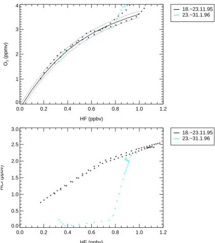
As an example, the derivation of the early winter reference function in 1995–1996 from HALOE profiles inside the early vortex is discussed. In this winter HALOE vortex profiles were available at the end of November. At this time of the winter, the APSCwas
20
negligible. No deviation from the unperturbed HCl/HF relation was found. Therefore, no activated chlorine compounds and thus no ozone loss can be expected. At the end of January (Fig.1, bottom panel) one profile inside the vortex boundary region indicates strong chlorine activation noticeable as a change in the HCl/HF relation in correspon-dence which a large APSCduring January. But still, no changes in the O3/HF relation 25
are detected (Fig.1, top panel). Changes in the O3/HF relation due to isentropic
mix-ing are not expected durmix-ing December and January, because at that time the vortex was already very strong. Therefore, this single January profile still describes the
chem-ACPD
4, 2167–2238, 2004
Ozone loss and chlorine activation in
the Arctic winters 1991–2003 S. Tilmes et al. Title Page Abstract Introduction Conclusions References Tables Figures J I J I Back Close
Full Screen / Esc
Print Version Interactive Discussion
© EGU 2004 ically undisturbed O3/HF relation. Of course, the HCl-tracer relation decreases much
faster than the O3-tracer relation, because chlorine activation occurs on much shorter time scales than ozone loss. However, in this winter ozone loss causes deviation from the derived early winter reference function that is less than its range of uncertainty. The fact that in 1996 – in spite of the early vortex having been cold and strong – no
signif-5
icant ozone loss occurred during January may be explained by the very small amount of sunlight that has illuminated the early vortex. The delayed occurrence between chlo-rine activation and ozone loss is further discussed below, considering the tracer-tracer correlation during spring.
In the following, the derivation of the early winter reference function from balloon
10
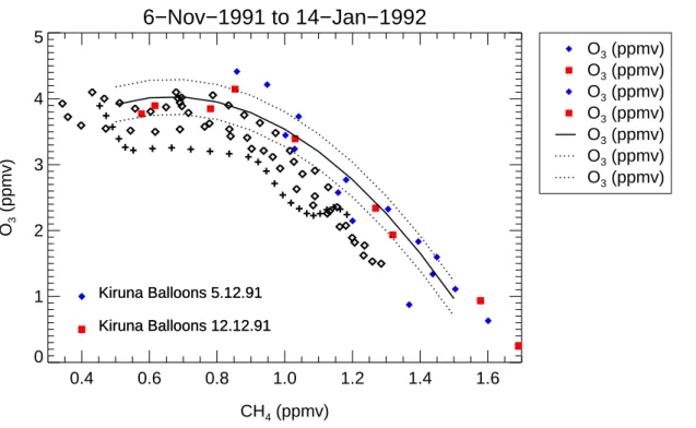
observations in 1991–1992, 1999–2000 and 2002–2003 is briefly described. For winter 1991–1992, the early winter reference function was derived from measurements of ozone and N2O made by cryosampler measurements (Schmidt et al.,1987) on 5 and 12 December 1991, respectively. The O3/N2O profiles were transformed to O3/CH4
with the N2O/CH4 relationship from Engel et al. (1996), see M ¨uller et al. (2001). To
15
derive the O3/HF reference function the O3/CH4 relation was converted using the
CH4/HF relation derived from HALOE observations for the winter 1991–1992 (Table1).
The vortex started forming in November 1991. One HALOE profile was found inside the early vortex at the beginning of November, with low ozone mixing ratios compared to profiles inside the vortex measured in January (see Fig. 2, black asterisks). At
20
that time the vortex was not well developed and mixing in of air masses from out-side the early vortex was still possible. Therefore, the low ozone mixing ratios ob-served in November increased until the vortex became fully isolated in December. The HALOE profiles in January 1992 scatters below the derived reference relation for about 1.2 ppmv (see Fig.2). Thus ozone loss have already occurred during January 1992,
25
corresponding to a small detected area of possible PSC existence at the beginning of January (see Fig.6). In contrast to the winter 1995–1996, ozone loss during January 1992 was much stronger although APSCin January 1995–1996 was even larger than in January 1991–1992. This shows that ozone loss is influenced by more than APSC as
ACPD
4, 2167–2238, 2004
Ozone loss and chlorine activation in
the Arctic winters 1991–2003 S. Tilmes et al. Title Page Abstract Introduction Conclusions References Tables Figures J I J I Back Close
Full Screen / Esc
Print Version Interactive Discussion
© EGU 2004 further discussed in Sect. 6.
In winter 1999–2000 again no HALOE observations were available inside the early vortex to derive the early winter reference function. Fortunately, during the SOLVE-THESEO 2000 campaign two balloon flights were conducted inside the early vortex, the OMS (Observations of the Middle Stratosphere) in-situ flight on 19 November 1999 and
5
the OMS remote flight on 3 December 1999 (M ¨uller et al.,2002). HF measurements were only available from the MkIV instrument on the OMS-remote flight. Thus, these data were used to derive the O3/HF reference function for this winter. Two early winter
reference functions were derived using CH4 as the long-lived tracer, one was derived using the OMS-in-situ measurements and the second using the OMS-remote flight
10
measurements (M ¨uller et al., 2002). For 2002–2003, MkIV balloon observations in mid-December 2002 (Toon et al.,1999) were used to derive the early winter reference function (Tilmes et al.,2003a).
The early winter reference functions of the winters 1994–1995 and 2002–2003 were derived from measurements at a time, when the vortex was already developed. Before
15
this time, a large area of PSCs was already detected and some activation of chlorine already occurred (Tilmes et al.,2003a). HALOE measurements in January 1994–1995, show strong deviations of the HCl/HF relations at the time when the reference function was deduced. Rex et al.(2003b) andGoutail et al. (1999) reported large ozone loss rates for January 1995. These losses may have already result in a small decrease of
20
the O3/HF relation before the reference function was deduced. Therefore, these ozone
losses cannot be included in the calculations below.
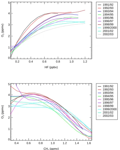
The derived ozone-tracer early winter reference functions for ten out of twelve years are shown in Fig.3.
The ozone-tracer relation in the early winter has its own characteristics each year,
25
mainly due to inter-annual differences in polar vortex development and not due to chemical loss (Manney et al.,2003b). Thus, it is not possible to use one single refer-ence function for all years. Year to year variations are also possible due to the changes of mixing ratios of the long-lived tracer used. Especially the increase of HF from 1991
ACPD
4, 2167–2238, 2004
Ozone loss and chlorine activation in
the Arctic winters 1991–2003 S. Tilmes et al. Title Page Abstract Introduction Conclusions References Tables Figures J I J I Back Close
Full Screen / Esc
Print Version Interactive Discussion
© EGU 2004 to 2003 should have an influence on the O3/HF reference function.
Therefore, two early winter reference functions, one for winter 1997–1998 and an-other for 2000–2001, were constructed from a climatology of all HALOE profiles that were measured inside the early vortex over the ten year period between 1992 and 2002. Actually, measurements inside the early vortex are available for six winters
5
(1992–1993, 1993–1994, 1994–1995, 1995–1996, 1998–1999 and 2001–2002). The HALOE O3/HF and O3/CH4profiles are corrected for the growth rate of HF and CH4, respectively, between each single year and the year 1997–1998 (2000–2001). The CH4 growth was taken from the tropospheric growth rate derived by Simpson et al. (2002). The HF growth rate was deduced from the HALOE HF/CH4 relationships
10
(Table 1) (Tilmes, 2003). No correction was applied to ozone, because ozone was relatively constant during the 1990s in northern latitudes (WMO,2003). The O3/CH4
and O3/HF profiles inside the early vortex of the six years transformed in this way are
used to construct reference functions for 1997–1998 and 2000–2001 determined from all available HALOE measurements inside the early vortex. Thus, for the winter 1997–
15
1998 and 2000–2001 in each case two early winter reference relations were derived, one using HF as the long-lived tracer and one using CH4(Tables2and3).
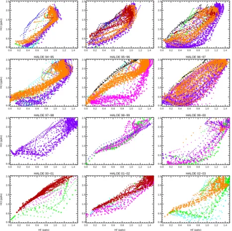
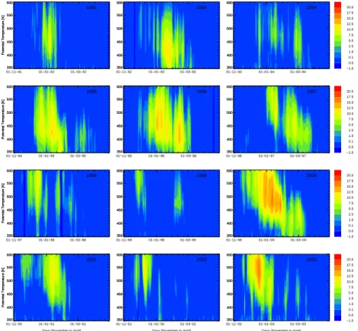
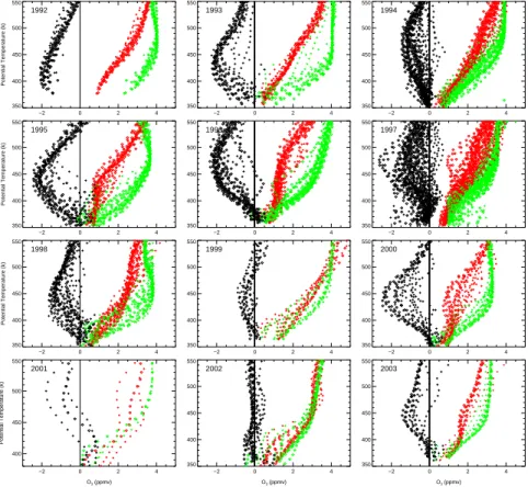
3.2. Tracer-tracer development during twelve Arctic winters
Active chlorine inside the polar vortex causes chemical ozone loss. Chlorine activation in the Arctic lower stratosphere may be identified as a strong reduction of HCl
com-20
pared to normal values. Therefore, using measurements made by HALOE, the evolu-tion of the chlorine chemistry can be inferred from the development of the HCl-tracer relation during each year. The evolution of HCl-tracer relation and O3-tracer relation is analysed for each of the twelve observed winter periods (Figs.4and5). The tempera-tures thus control the activation of chlorine and consequently the chemical destruction
25
of ozone. If temperatures are sufficiently low PSCs can occur in the polar stratosphere. Therefore, APSCis used here to analyse the interaction between meteorology and de-velopment of tracer-tracer relationship for each winter (Fig.6). Further, a division into
ACPD
4, 2167–2238, 2004
Ozone loss and chlorine activation in
the Arctic winters 1991–2003 S. Tilmes et al. Title Page Abstract Introduction Conclusions References Tables Figures J I J I Back Close
Full Screen / Esc
Print Version Interactive Discussion
© EGU 2004 cold, moderately cold and warm winters is carried out.
– 1991–1992:
The cold vortex in winter 1991–1992 was disturbed by several warming pulses between November and February (Naujokat et al.,1992). The threshold temper-ature for PSCs was only reached during January. Therefore, significant ozone
5
depletion can be expected starting in January 1992. During March the tempera-tures at the north pole steadily increased and the vortex finally broke down at the end of April (Naujokat et al.,1992). In February and at the beginning of March very low HCl mixing ratios are clearly noticeable and strong chlorine activation (Fig.4) occurred in the lower stratosphere (below ≈420 K).
10
By April, the HCl levels have increased towards unperturbed values, especially in altitudes below ≈420 K. The vortex became steadily weaker during April. From February up to the beginning of April a homogeneous moderate deviation from
O3/HF reference functions was occurring.
– 1992–1993:
15
The vortex in winter 1992–1993 was cold and nearly undisturbed until the end of January. A strong minor warming in February shifted the cold air (with low ozone values) towards Europe. This, together with a blocking anticyclone in the troposphere, led to low total ozone values over Europe in February (Naujokat and Labitzke,1993). Conditions for chemical ozone loss were reached, because of the
20
low stratospheric temperatures (Fig. 6). Unfortunately, no measurements were taken inside the vortex in February, but HCl measurements inside the outer part of the vortex boundary region indicate a strong chlorine activation in February at lower altitudes (Fig.4, small green crosses). Temperatures started rising in March and the final break-up of the vortex occurred around 10 April. At that time HCl
25
levels have recovered to unperturbed values. Strong (homogeneous) deviation from the O3-tracer reference function is obvious in March and April (Fig.5). Until the end of April, the deviation from the O3/HF reference function does not further
ACPD
4, 2167–2238, 2004
Ozone loss and chlorine activation in
the Arctic winters 1991–2003 S. Tilmes et al. Title Page Abstract Introduction Conclusions References Tables Figures J I J I Back Close
Full Screen / Esc
Print Version Interactive Discussion
© EGU 2004 change inside the remaining parts of the vortex.
– 1993–1994:
The early vortex in winter 1993–1994 was slightly disturbed in November, Decem-ber and January (Naujokat et al.,1995a). Owing to the warming over Europe in February, the vortex was split most of the time. At the end of February and the
5
beginning of March, the vortex air masses cooled down again and temperatures were below the threshold for the existence of PSCs for a few days (Fig. 6). A small decrease of HCl in February is noticeable from the HCl/HF relation (Fig.4). Afterwards HCl strongly decreased during March (HCl mixing ratios were below 0.1 ppbv for HF mixing ratios below 0.7 ppbv). During April the HCl levels quickly
10
increased while the vortex became weaker. In March and April moderate devia-tions from the O3/HF reference function became noticeable (Fig.4), although the chlorine activation in March seemed to be quiet pronounced.
– 1994–1995:
The vortex in 1994–1995 formed early and was very cold and strong especially
15
between mid-December and mid-January. A large APSC was deduced for the whole of January 1995. Owing to a warming event in February the vortex was displaced towards Siberia but did not break. The temperatures of the cold centre of the vortex towards Siberia were low enough for PSC formation until 10 February (Naujokat et al., 1995b). Record low temperatures were reached again in the
20
lower stratosphere in March (Naujokat et al., 1995b). In April the vortex split and one part rapidly weakened and disintegrated over eastern Asia. The main vortex centre vanished more slowly. As in winter 1992–1993, a strong decrease of HCl mixing ratio in the outer part of the vortex boundary region was observed by HALOE in February. Although the chlorine activation in March was not as
25
strong as in the previous winter 1993–1994, much stronger deviations from the O3-tracer reference relation in March were observed. During April the HCl levels have increased towards unperturbed values.
ACPD
4, 2167–2238, 2004
Ozone loss and chlorine activation in
the Arctic winters 1991–2003 S. Tilmes et al. Title Page Abstract Introduction Conclusions References Tables Figures J I J I Back Close
Full Screen / Esc
Print Version Interactive Discussion
© EGU 2004
– 1995–1996:
The winter 1995–1996 was the coldest recorded by the US National Meteorol-ogy Center (NMC) in 18 years (Manney et al., 1996). Since December 1995, the stratospheric temperatures in the Arctic were below the PSC threshold until March. The final warming began in early March. Measurements taken by HALOE
5
in the vortex are available for the first part of March and the first part of April. The strongest chlorine activation in March for this twelve-year overview was observed. In April, HCl levels have almost completely recovered to unperturbed values. The deviation from the early winter reference function O3/HF is the same for March
and April, so that in April no further ozone loss was identified between March and
10
April.
– 1996–1997:
In winter 1996–1997, the polar vortex formed in November. It was strongly dis-turbed at the end of November and reformed again during December. Before the vortex was fully established at the end of December, horizontal mixing between
15
air from inside and outside the vortex occurred and the minimum temperature remained above the PSC threshold of ≈195 K. After the reformation, the vortex was very cold and strong. At the 475 K potential temperature level, the lowest temperatures in an 18-year data set were reached in this year in March and April (temperatures were below the PSC threshold until the beginning of April) inside
20
the vortex core (Coy et al.,1997). In March, the vortex core was small and strong whereas the boundary region was wide. PSC occurrence was not possible before January therefore no chlorine activation and thus no ozone loss can be expected in November and December 1996. Until the end of March the temperatures were low enough for PSC existence (Fig. 6). During mid-February, this potential for
25
chemical ozone loss was enhanced by significant denitrification (Kondo et al., 2000). Deviations from the O3-tracer early winter reference function are sepa-rated into two parts. The chlorine activation is also rather inhomogeneous with the strongest decrease of HCl inside the vortex core, except for one profile inside
ACPD
4, 2167–2238, 2004
Ozone loss and chlorine activation in
the Arctic winters 1991–2003 S. Tilmes et al. Title Page Abstract Introduction Conclusions References Tables Figures J I J I Back Close
Full Screen / Esc
Print Version Interactive Discussion
© EGU 2004 the outer vortex, measured in the second part of March (Fig.4, small purple plus
sign). The strongest April decrease of HCl mixing ratio was observed in this year, because the vortex remained intact for an extremely long period.
– 1997–1998:
The vortex in 1997–1998 was slightly disturbed throughout the whole winter. The
5
final warming began in the middle of March (Pawson and Naujokat,1999). Mini-mum temperatures were low enough to activate HCl during December and during January (Fig.6). Moderate chlorine activation was observed by HALOE in March and only small deviations from the reference function for O3-tracer occurred. In that winter HALOE data are only available for March inside the polar vortex.
10
– 1998–1999:
The winter 1998–1998 was unusually warm due to a major stratospheric warming in mid-December (Manney et al.,1999). The vortex in 1998–1999 was very weak and disturbed. Almost no changes in the HCl/HF relation occurred, owing to a small APSCand thus, very little chlorine activation at the end of February. However,
15
small deviations from the O3/HF early winter reference function were found (see
discussion below).
– 1999–2000:
In 1999–2000 the Arctic stratosphere was very cold from the middle of November to late March (Manney and Sabutis,2000). The lowest values of the February HCl
20
mixing ratios for any of the observed years were reached, owing to the largest APSC during January in the observed period. HCl mixing ratios are comparable to the low mixing ratios in March 1996. In March 2000, a slight recovery of HCl levels towards unperturbed values became noticeable, with a total recovery at the end of April. The small deviation from the early winter reference function HF/O3
25
in February strongly increased in March up to April.
ACPD
4, 2167–2238, 2004
Ozone loss and chlorine activation in
the Arctic winters 1991–2003 S. Tilmes et al. Title Page Abstract Introduction Conclusions References Tables Figures J I J I Back Close
Full Screen / Esc
Print Version Interactive Discussion
© EGU 2004 The vortex in 2000–2001 developed during October and November 2000. A
strong Canadian warming at the end of November greatly disturbed the vortex. An undisturbed cold period followed from late December until mid-January. Af-terwards, a major warming broke down the vortex in mid-February. During this warming, the vortex drifted over central Europe for a few days and PSC conditions
5
were reached due to a short-term cooling of the vortex. The vortex re-established in March and lasted until April. Figure 4 displays strong chlorine activation in February 2001. From March to April HCl levels totally recovered towards normal values. In the ozone-tracer relation in February 2001 one profile inside the outer vortex indicates a significant deviation from the early winter reference function. In
10
March and April the early winter reference function is certainly not valid any more, owing to the temporary break-up of the vortex in February, and ozone-tracer pro-files scatter above the derived function. Therefore, the TRAC technique cannot be applied to ozone-tracer profiles in March and April.
– 2001–2002:
15
The winter 2001–2002 was a very warm winter. Although the temperatures at the end of November reached a record minimum for the period 1979–2001, a strong warming in the second half of December occurred so that the vortex significantly weakened. After the vortex was re-established in January, it was weak and warm until it broke down in May. Very little chlorine activation is noticeable at the end of
20
March 2002 (Fig.4) and very little deviation from the O3/HF early winter reference
relation is apparent at the end of April.
– 2002–2003:
In this winter the polar vortex formed in November 2002. It was characterised by very low temperatures in the early vortex and chlorine activation already in
25
mid-December 2002. APSC was largest in December for the entire lifetime of the vortex. Afterwards, temperatures increased around mid-January and the vortex split two times, once in January and once in February. Only a small APSC was
ACPD
4, 2167–2238, 2004
Ozone loss and chlorine activation in
the Arctic winters 1991–2003 S. Tilmes et al. Title Page Abstract Introduction Conclusions References Tables Figures J I J I Back Close
Full Screen / Esc
Print Version Interactive Discussion
© EGU 2004 derived for the following month. Some chlorine deactivation was deduced from the
HALOE measurements in the vortex in February. In April, HCl had recovered, thus chlorine was completely deactivated. The strongest deviation from the ozone-tracer reference appeared for the profiles in February, and for one profile in April. A detailed analysis of this winter using the TRAC method is described in (Tilmes
5
et al.,2003a).
To summarise the temperature conditions for winters between 1991–1992 and 2002– 2003, five winters are characterised as being cold (1992–1993, 1994–1995, 1995– 1996, 1996–1997 and 1999–2000). These winters show a strong decrease of the HCl mixing ratio in the HCl/HF relation in spring and strong deviations of O3-tracer profiles
10
from the early winter reference function. For the cold winters the daily APSCaverage in 400–500 K between January and March is above 3*106km2(shown below in Sect. 6). Moderate deviations from the O3/HF reference were found in 1991–1992, 1993–1994,
1997–1998, 2000–2001 and 2002–2003. These winters indicating a more frequently disturbed vortex are characterised as moderately cold. The daily APSCaverage is ≈1–
15
2*106km2. The winters 1998–1999 and 2001–2002 are warm with very little chlorine activation and very little deviation from the early winter ozone-tracer reference function. The value of the daily APSCaverage does not exceed 0.5*106km2for these very warm winters.
4. Ozone loss profiles and column ozone loss
20
The chemical ozone loss calculated using the TRAC method should be interpreted as the total amount of destroyed ozone in a period between the time of the early winter reference function and the time of the investigated profile. In this section, calculated local ozone loss profiles in February/March each year are presented, as well as the monthly average column ozone loss over the course of the entire winter for two different
25
ACPD
4, 2167–2238, 2004
Ozone loss and chlorine activation in
the Arctic winters 1991–2003 S. Tilmes et al. Title Page Abstract Introduction Conclusions References Tables Figures J I J I Back Close
Full Screen / Esc
Print Version Interactive Discussion
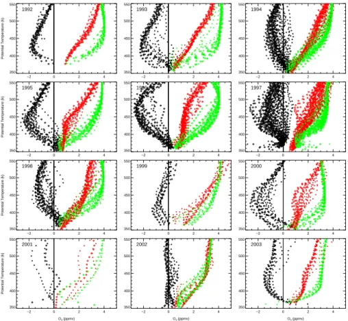
© EGU 2004 4.1. Vertical ozone loss profiles
For each year, the ozone loss profiles differ with respect to the altitude range where ozone loss occurs, the maximum local ozone loss, the altitude where this maximum loss occurs and the extent of homogeneity of the distribution inside the vortex. Vertical ozone loss profiles are calculated using both HF (Fig.7) and CH4(Fig.8) as the
chemi-5
cally long-lived tracers. These ozone loss profiles (black symbols) are calculated as the difference between the actually measured ozone concentration O3 (red symbols) and the corresponding ozone proxy ˆO3 (green symbols) (e.g. M ¨uller et al., 1996; Tilmes, 2003).
In all winters considered, significant ozone loss arose mainly in an altitude range
10
between 380 and 550 K. At altitudes below 380 K the uncertainty of calculated ozone loss profiles increased in most winters, because of the increasing dynamic variability, that is the influence of mixing processes.
The amount of ozone destroyed at different altitudes and, therefore, the shape of the vertical ozone loss profiles depends on the different meteorological conditions inside
15
the polar vortex for each winter. The maximum of the vertical ozone loss profile (in mixing ratio) and the corresponding altitude range (in potential temperature) is shown in Table4for March (or February in the year 2001 and 2003) of each year.
The results derived using two different tracers are within the combined uncertainties for each year. To perform a comparison between the different years, the average of
20
the maximum ozone loss of the two different long-lived tracers is calculated (Table 4, column 6). The strongest local ozone loss of all the years considered, about 2.4 ppmv in 1995–1996 and 2.5 ppmv 1996–1997, was found in the altitude range from about 450–490 K. In the cold winters of 1994–1995 and of 1999–2000 the maximum of local ozone loss profiles was similarly strong in the altitude range from about 410–460 K.
25
In March 1992 and 1993 local ozone loss is also rather strong, 2.0 ppmv in 1992 and 2.2 ppmv in 1993 at very low altitudes in 390–460 K. Winters termed moderately cold, in the section above, 1991-1992, 1993-1994, 1997-1998 and 2001–2002, show local
ACPD
4, 2167–2238, 2004
Ozone loss and chlorine activation in
the Arctic winters 1991–2003 S. Tilmes et al. Title Page Abstract Introduction Conclusions References Tables Figures J I J I Back Close
Full Screen / Esc
Print Version Interactive Discussion
© EGU 2004 ozone loss of about 1.5 ppmv, except for the winter 1991-1992. (The reason for the
relatively strong ozone loss in 1991–1992 is discussed below). In 2000–2001 local ozone loss reached 1.7 ppmv from profiles inside the outer vortex in February only, whereas the local ozone loss profiles inside the vortex core did not exceed 1.0 ppmv in February 2000–2001 (Fig.7). In the warm winters, 1998–1999 and 2001–2002, the
5
local ozone loss is 1.0 ppmv and 0.4 ppmv, respectively.
As well as the value of the maximum itself, the altitude ranges and the width of the peak of the maximum ozone loss differs from winter to winter in correspondence to the location of APSCduring the winter. These factors control the amount of column ozone loss calculated by the vertical integration of the ozone loss profile.
10
In some years 1991–1992, 1992–1993, 1999–2000, 2002–2003, the ozone loss pro-files taken inside the vortex core are very homogeneous (Fig.8). This is the result of an isolated vortex core with homogeneous ozone loss.
For 1993–1994, 1994–1995, 1995–1996 and 1997–1998, a few profiles of ozone loss indicate a somewhat smaller deviation from the reference function inside the
vor-15
tex core but the majority of profiles inside the vortex core are homogeneously dis-tributed. In 1993–1994 and 1994–1995 a warming in February disturbed the isolated vortex. The vortex shifted off the pole and the cold region was near the edge of the vortex. At this time rapid ozone destruction occurred at the vortex edge (Manney et al., 2003a). The vortex in 1995–1996 and 1997–1998 was already weakening at the end
20
of February and broke down in March. The ozone loss profiles∆O3in 1996–1997 are separated in two distinct parts with moderate loss inside the entire vortex and strong loss in the vortex core (Tilmes et al.,2003b).
The meteorological developments during various winters, described above, may be responsible for inhomogeneous temperature distributions inside the vortex and,
there-25
fore, are responsible for the inhomogeneities in ozone destruction inside the entire vortex. For for the most years considered here, the calculated ozone loss profiles for the outer vortex (plus signs in Figs.7and8) show less ozone loss than the profiles in the vortex core. The temperatures inside the outer vortex are generally not as low as
ACPD
4, 2167–2238, 2004
Ozone loss and chlorine activation in
the Arctic winters 1991–2003 S. Tilmes et al. Title Page Abstract Introduction Conclusions References Tables Figures J I J I Back Close
Full Screen / Esc
Print Version Interactive Discussion
© EGU 2004 inside the vortex core and, therefore, less ozone loss occurred inside the outer vortex
than inside the vortex core. In some years (March 1994–1995, 1997–1998, 1998–1999 and February 2000–2001) very few profiles show slightly stronger deviations from the reference relation and, therefore, stronger ozone loss inside the outer vortex than in-side the vortex core. This is possible, because the exposure to sunlight may be longer
5
inside the outer vortex than inside the vortex core, due to the location of the outer vor-tex more towards lower latitudes. Further discussion of the differences between ozone loss inside the vortex core and the outer vortex is given below in the next section. 4.2. Column ozone loss
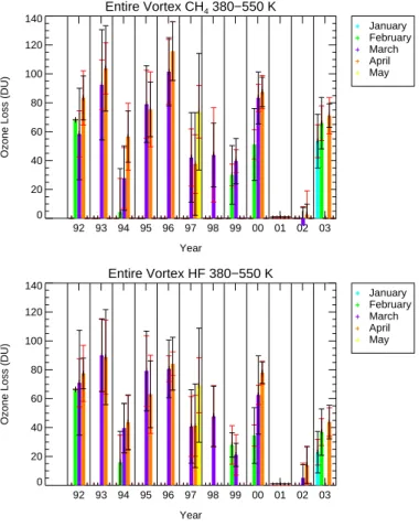
Column ozone loss for a twelve years period was derived by integrating the vertical
10
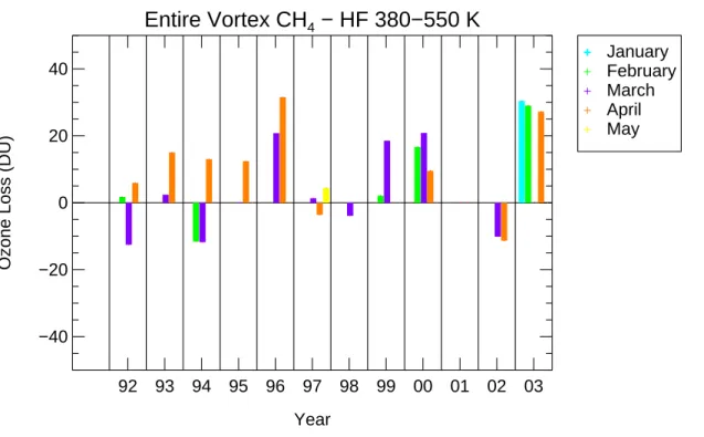
ozone loss profiles (see Appendix A). This value constitutes a good approximation of the total amount of ozone loss over the entire column of ozone if the vertical integration is extended over a sufficiently large vertical range (≈380–550 K). In this paper, the monthly average column ozone loss is analysed for altitude ranges between 380 and 550 K and between 400–500 K. Further, a comparison of results of different parts of the
15
polar vortex was performed as well as comparison between the results using different long-lived tracers.
Tables5 and6 summarise the column ozone loss in 380–550 K and in 400–500 K, respectively, averaged over different months, February, March, April and May (May only in winter 1996–1997), calculated for each year if measurements are available. In
20
February 2000–2001, for two of three profiles measured inside the entire vortex ozone loss was found only in altitudes above ≈450 K (Figs. 7 and 8). These two profiles scatter above the estimated early winter reference function in altitudes below 450 K and would wrongly increase the calculated ozone loss. Thus, for this winter the column ozone loss was calculated for the altitude range between 450 and 500 K only. In Fig.9
25
results for the entire vortex are shown, calculated for the altitude range of 380–550 K. The uncertainty of the mean column ozone loss is described by two parameters. The uncertainty which arises solely due to the uncertainty of the early winter reference
ACPD
4, 2167–2238, 2004
Ozone loss and chlorine activation in
the Arctic winters 1991–2003 S. Tilmes et al. Title Page Abstract Introduction Conclusions References Tables Figures J I J I Back Close
Full Screen / Esc
Print Version Interactive Discussion
© EGU 2004 function is shown as a red error bar in Fig.9. The standard deviation of the column
ozone loss deduced from the individual profiles, is shown as a black error bar.
The uncertainty of the early winter reference function is about 15–25 DU in the alti-tude range of 380–550 K (Table5) depending on the scatter of profiles inside the early vortex from which the reference function was derived. If there is little variability of the
5
mixing ratios of tracers inside the early vortex, the error in the results is smaller than 10 DU. This is the case in the year 1995–1996 using HF as the long-lived tracer and in 1998–1999 using CH4 as the long-lived tracer. Differences of the uncertainties of the results derived using two different long-lived tracers in one year is possible, due to differences in the random error of the different tracers used. If the early winter
refer-10
ence function was derived using only one profile, as it is the case in 1999–2000 and 2001–2002, information about the variability of the mixing ratios of tracers inside the early vortex are not included, and the estimated error may be underestimated.
For March 1997 the standard deviation of averaged column ozone loss is larger compared to the other winters and is much larger than the early winter reference error
15
(Fig. 9). At this time, the vortex is divided into two parts, a part with strong ozone loss and a part with moderate ozone loss (McKenna et al.,2002;Tilmes et al.,2003b). The ozone loss in March 1996–1997 is spatially much more inhomogeneous than the ozone loss observed in all the other winters investigated here (Fig.7).
The error which arises owing to the early winter reference function is significantly
20
smaller in an altitude range of 400–500 K than in 380–550 K (Tables5 and 6). Here, calculated ozone loss for the cold, moderately cold and warm winters between the 400– 500 K level is summarised. In the following, the average between the results using CH4 and HF as the long-lived tracers are considered. In 1992–1993, 1994–1995, 1995– 1996 and 1999–2000 column ozone loss is 60–80 DU between the 400–500 K level.
25
The maximum of the column ozone loss in this twelve-year study was obtained for the winters 1992–1993 and 1995–1996. In 1996–1997 the strongest mean ozone loss was reached in May (48 DU in the 400–500 K level). Although the winter 1996–1997 was cold, the mean column ozone loss for this winter (47±17 DU inside the vortex
ACPD
4, 2167–2238, 2004
Ozone loss and chlorine activation in
the Arctic winters 1991–2003 S. Tilmes et al. Title Page Abstract Introduction Conclusions References Tables Figures J I J I Back Close
Full Screen / Esc
Print Version Interactive Discussion
© EGU 2004 core in the 400–500 K level in April) is comparable with the results of the moderate
winters, because of the inhomogeneity of the ozone loss in the vortex. Nonetheless, the maximum ozone loss locally of this winter is comparable with results of the cold winters (Fig.7) .
The moderately cold winters 1991–1992, 1994–1995,1997–1998 and 2002–2003
5
reach a mean column ozone loss between 31 DU (in winter 1994–1995) and 57 DU (in winter 1991–1992) inside the vortex core in March. (Results of winter 2002–2003 using CH4as the long-lived tracer are excluded, due to uncertain data, as discussed below). In 2000–2001, mean column ozone loss was deduced for February in 450–500 K, as described above. Only 10 DU were calculated for the entire vortex. Nevertheless, the
10
maximum column ozone loss reached 20±4 DU and 21±6 DU using HF and CH4 as the long-lived tracers for one profile inside the outer vortex in 450–500 K. In the warm winter 1998–1999 ozone loss still reaches 25±10 DU derived for an altitude range of 400–500 K from profiles inside the entire vortex and 21±10 DU for profiles inside the vortex core. Inside the entire vortex in March 2002 no ozone loss is diagnosed with the
15
TRAC technique within the uncertainty of the early winter reference function.
The exact mean calculated column ozone loss differs depending on whether HF or CH4is used as the long-lived tracer. Further, ozone loss differs depending whether the vortex core or the entire vortex is considered. In Fig.10, the difference between the ozone loss derived with the two long-lived tracers are shown.
20
The differences between the results are ≈10–20 DU for most of the observed years and are similar for the entire vortex and the vortex core (not shown). The smallest differences are calculated for the winter 1996–1997 and 1997–1998 (below 5 DU). The difference of the early winter reference functions using the two different long-lived tracer are mostly responsible for the different results. In most observed years the results
ob-25
tained using CH4as the long-lived tracer agree with those using HF inside the uncer-tainty introduced by the unceruncer-tainty of the reference function.
In some years, ozone loss calculated employing CH4 as the long-lived tracer has a tendency towards larger ozone loss toward the end of the winter compared to HF
ACPD
4, 2167–2238, 2004
Ozone loss and chlorine activation in
the Arctic winters 1991–2003 S. Tilmes et al. Title Page Abstract Introduction Conclusions References Tables Figures J I J I Back Close
Full Screen / Esc
Print Version Interactive Discussion
© EGU 2004 (Fig.9). Especially in March 1996, the results differ by more than 30 DU for the entire
vortex. In winter 2002–2003 results derived using CH4 as the long-lived tracer are significantly larger (25–30 DU) than using HF during the entire winter period. The CH4 mixing ratios inside the Arctic vortex at altitudes below about 450 K may be problematic in these years, due to signal saturation problems. Such problems are also discussed for
5
the winter 1999–2000 byM ¨uller et al.(2002) and may be responsible for the differences in 2002–2003 (Tilmes et al., 2003a). Therefore, results derived employing CH4 as the long-lived tracer are not discussed in Tilmes et al. (2003a). Also, the significant uncertainties in March 1996 may be explained by this problem.
Inside the outer vortex, the mean column ozone loss is in most cases less than inside
10
the vortex core (Fig.11). The vortex core usually is colder than the outer vortex and, thus, the extent of ozone loss is expected to be stronger, as described above. This effect is very strong for the winters 1991–1992, 1992–1993, 1996–1997, 1999–2000 and 2002–2003. However, in some years the ozone loss is insignificantly greater inside the outer vortex than inside the vortex core (in April 1992, 1994 and 1995, February
15
and March 1999 and February 2001). As discussed above, this is possible because the exposure to solar radiation may be longer inside the outer vortex than inside the vortex core, which causes stronger ozone loss. Further, in some years the standard deviation for profiles in the outer vortex is significantly larger than inside the vortex core (1992–1993, 1994–1995, 1995–1996 and 1999–2000) (see Tables5and6). That
20
is because the ozone loss inside the outer vortex was much more inhomogeneous than in the vortex core in these winters. These inhomogeneities may be caused by inhomogeneous temperature distributions inside the outer vortex.
5. Comparison with ozone loss estimates using different methods
The results deduced here using the TRAC method are compared with published results
25
obtained by different methods for the determination of chemical ozone loss. Chemical ozone loss in the Arctic vortex in the past decade was estimated by a variety of methods
ACPD
4, 2167–2238, 2004
Ozone loss and chlorine activation in
the Arctic winters 1991–2003 S. Tilmes et al. Title Page Abstract Introduction Conclusions References Tables Figures J I J I Back Close
Full Screen / Esc
Print Version Interactive Discussion
© EGU 2004 for different winters (Harris et al.,2002;Newman et al.,2002). However, a comparison
between the different ozone loss estimates is only meaningful, if the figures compared are determined for exactly the same conditions (Harris et al.,2002).
Column ozone loss from the SAOZ/REPROBUS approach (Goutail et al.,1999; De-niel et al.,1998; Lef `evre et al.,1998), was estimated for a period from December to
5
March/April for the winters 1993–1994 to 2002–2003 (Goutail et al.,2000,2003). The TRAC technique estimates ozone loss between the time when the reference function was derived and the time when HALOE measurements are available in March/April. The early winter reference function in winter 1993–1994 was derived from observa-tions at the end of November and at the beginning of January. During these two month
10
no ozone loss was found. To compare the results, ozone loss from SAOZ is also considered for the period between January and March 1994. Considering different al-titudes had little impact on the total column ozone loss. In this winter, SAOZ estimated ≈10% ozone loss in December (Goutail et al.,2003) and ≈7% between January and March. If an average of 441 DU is taken from the inert tracer simulations in March 1994
15
(pers. comm., F. Goutail, 2004) 31 DU ozone loss are estimated for the period between January and March 1994 from SAOZ (Table 7), which agrees well with accumulated ozone derived from HALOE measurements using the TRAC technique.
In winter 1994–1995, the early winter reference function was derived in mid-January. Therefore, SAOZ ozone loss is estimated for the time period between mid-January
20
and March (Goutail et al.,2003) (≈21% or 95 DU, where 452 DU is the approximated passive ozone). This result is somewhat greater than derived from HALOE, although inside the range of uncertainty (Table 7). The ozone loss derived using the Match technique (Rex et al.,1998;Schulz et al.,2000) for the same winter but for the time period between 1 January and March 1995, in 370–700 K, is more than 40 DU larger
25
(127±14 DU) than that from HALOE (in 380–550 K). Like SAOZ, the Match technique estimated strong ozone loss during the first two weeks in January. Because the tempo-ral evolution of ozone destruction estimated by SAOZ and Match coincides quiet well (Rex et al.,1998), we assume that about 12% of 36±4% derived by Match occurred
ACPD
4, 2167–2238, 2004
Ozone loss and chlorine activation in
the Arctic winters 1991–2003 S. Tilmes et al. Title Page Abstract Introduction Conclusions References Tables Figures J I J I Back Close
Full Screen / Esc
Print Version Interactive Discussion
© EGU 2004 during the first half of January. This results in accumulated ozone loss of 24±4%
(108±18 DU) estimated from Match results, which agrees with HALOE results with the range of uncertainty (Table7).
The early winter winter reference function in 1995–1996 was derived from both November and January profiles. As for 1993–1994 no ozone loss was found during
5
these two month. SAOZ accumulated ozone loss in winter 1995–1996 between mid-January and March is ≈20% (83 DU). This value is in good agreement with HALOE results. For 1996–1997 the result from SAOZ agrees with the largest ozone loss cal-culated by HALOE inside the vortex core (90–110 DU), but averages do not agree.
In winters 1997–1998 and 1998–1999 results of SAOZ and HALOE data agrees
10
within the considered uncertainty. The estimated ozone loss from SAOZ in winters 1999–2000, 2001–2002 is ≈20 DU larger than derived here from HALOE.
The column ozone loss from UARS microwave limb sounder (MLS) measurements for the winters 1991–1992 to 1997–1998 was calculated for above 100 hPa (Manney et al.,2003a). Therefore, the results are compared with HALOE results for the potential
15
temperature range 400–550 K (Table 8). The results of the two methods agree in so far as, with both techniques, the strongest ozone loss was found for the winters 1995– 1996 and 1992–1993. For the winters 1991–1992, 1992–1993, 1994–1995, the ozone losses determined from MLS data are about 10 DU smaller than the lower limit of the uncertainty range of those derived from HALOE data for profiles inside the entire
vor-20
tex. In 1995–1996 and 1997–1998 MLS results are smaller than those deduced from HALOE, but within the considered uncertainties of the HALOE results. In 1993–1994 values calculated from HALOE observations are insignificantly smaller (6 DU) than cal-culated from MLS observations inside the entire vortex. For 1996–1997 the average value of the entire vortex is in accordance with the MLS observations.
25
MLS values of column ozone loss are reported only for the height range above 100 hPa. The column ozone loss between the potential temperature levels 400–550 K deduced here based on HALOE measurements will not exactly correspond to a loss derived for a height range above 100 hPa, and may include some ozone loss at