Downscaling and projection of summer rainfall in Eastern China using a nonhomogeneous hidden Markov model

(1)

HAL Id: hal-02016597

https://hal.sorbonne-universite.fr/hal-02016597

Submitted on 12 Feb 2019

HAL is a multi-disciplinary open access

archive for the deposit and dissemination of sci-entific research documents, whether they are pub-lished or not. The documents may come from teaching and research institutions in France or abroad, or from public or private research centers.

L’archive ouverte pluridisciplinaire HAL, est destinée au dépôt et à la diffusion de documents scientifiques de niveau recherche, publiés ou non, émanant des établissements d’enseignement et de recherche français ou étrangers, des laboratoires publics ou privés.

Downscaling and projection of summer rainfall in

Eastern China using a nonhomogeneous hidden Markov

model

Lianyi Guo, Zhihong Jiang, Mei Ding, Weilin Chen, Laurent Li

To cite this version:

Lianyi Guo, Zhihong Jiang, Mei Ding, Weilin Chen, Laurent Li. Downscaling and projection of summer rainfall in Eastern China using a nonhomogeneous hidden Markov model. International Journal of Climatology, Wiley, In press, �10.1002/joc.5882�. �hal-02016597�

(2)

Accepted manuscript. Guo et al. 2018 International J. of Climatology https://doi.org/10.1002/joc.5882 page 1

Downscaling and projection of summer rainfall in Eastern China

using a nonhomogeneous hidden Markov model

Lianyi Guo1, Zhihong Jiang1*, Mei Ding2, Weilin Chen1, Laurent Li1, 3

1. Key Laboratory of Meteorological Disaster, Ministry of Education, Joint International Research Laboratory of Climate and Environment Change, Collaborative Innovation Center on Forecast and Evaluation of Meteorological Disasters, Nanjing University of Information Science &Technology, Nanjing 210044, China

2. Maanshan Meteorological Bureau, Maanshan 243000, China

3. Laboratoire de Météorologie Dynamique, CNRS, Sorbonne Université, Ecole Normale Supérieure, Ecole Polytechnique, Paris, France

* Corresponding author address: Prof. Zhihong Jiang, College of Atmospheric Sciences, Nanjing University of Information Science and Technology, 219 Ning Liu Road, Nanjing 210044, China. E-mail: zhjiang@nuist.edu.cn

(3)

Abstract

A nonhomogeneous hidden Markov model (NHMM) is used to stochastically simulate summer (June- August) daily precipitations in the middle and low reaches of the Yangtze River in Eastern China, with driving forcing from three global climate models (GCMs). Simulations cover the historical period from 1961 to 2005 and from 2006 to 2100 following the RCP4.5 scenario. The model is firstly evaluated against data from the regional observation network. Results show that NHMM effectively enhances the ability of GCMs in simulating summer daily rainfall in the region. For future projection at different time horizons of the 21st century, the spectral distribution of regional precipitations (in function of their intensity) shows consistent changes with a decrease of occurrence probability for light rain (< 10mm/day) and an increase for heavy rain (> 10mm/day). Among variables of interest, total precipitation (PRCPTOT), precipitation intensity (SDII), number of rainy days for daily precipitation exceeding 10mm (R10mm) and 95th percentile of precipitation (P95), all show a gradually increasing trend in the 21st century, and geographically an eastward gradient with smaller increase (or even weak decrease) for the west and larger increase for the east. It is noted that obvious changes occur in eastern region with 95% significance level, and PRCPTOT or R10mm increases by 40%~60% in the late 21st century. Further quantitative assessment is performed for global warming of 1.5℃ and 2℃. The half-degree additional warming makes R10mm change by -3.7%, 2.4% and 12.1% over western, central and eastern regions, respectively.

Key words: Nonhomogeneous hidden Markov model, Statistical downscaling, Daily

(4)

1 Introduction

The middle and low reach of the Yangtze River in Eastern China is strongly influenced by the Asian monsoon. The annual precipitation in this zone is about 1000mm and two-thirds fall in summer. The region suffers frequent extreme climate events causing serious losses of lives and properties. It is therefore important for us to investigate future evolution of such events under global warming. Furthermore, the 2015 Paris Agreement aims to limit the global warming to well below 2℃ above the pre-industrial and to pursue efforts to limit it to 1.5℃ (UNFCC, 2015). Particularly, the half-degree warming from 1.5°C to 2.0°C becomes an issue for international geopolitics, since some recent studies concluded that it may drastically augment the occurrence frequencies and impacts of extreme events (Schaeffer et al., 2012; Knutti et al., 2016).

Global climate model (GCM) which can well simulate large-scale climate variables is often used to make future climate change projection in China. However, GCM has shortcomings to well simulate regional climate, mainly due to its relatively coarse spatial resolution. It generally fails to reproduce mean and extreme precipitations (Jiang

et al., 2009; Xu et al., 2011; Jiang et al., 2012; Jiang et al., 2015; Yang et al., 2016).

Downscaling techniques are thus indispensable to transform outputs of GCM to reliable regional climate simulations. To do so, the statistical downscaling approach can be very appropriate, in particular, for simulating daily precipitation and with multiple realisations (Ben Alaya et al., 2015; Dayon et al., 2015; Jha et al., 2015; Ding et al.,

2016; Hundecha et al., 2016; Jones et al., 2016; Wu et al., 2016).

The nonhomogeneous hidden Markov model (NHMM) is a good candidate for climate downscaling. It was firstly used by Hughes et al. (1994) to construct a relationship between large-scale atmospheric information and regional precipitation.

(5)

This climate downscaling procedure is based on the hypothesis that the occurrence probability of local weather is determined by large-scale fields, NHMM being able to determine the transition of local meteorological pattern on a daily timescale. Many interesting results were reported in the literature on using NHMM to conduct climate downscaling in different regions and obtained good effect (Bates et al., 1998; Charles et

al., 1999; Greene et al., 2011; Tan et al., 2013; Cioffi et al, 2016). Fu et al. (2013a) used

NHMM to generate an ensemble of stochastic daily rainfall projections for 30 stations across south-eastern Australia. Robertson et al. (2004) applied NHMM to outputs of the global climate model ECHAM4.5 over Northeast Brazil and pointed out that the generated daily precipitation series have good statistical properties. Recently, we also applied NHMM to produce daily precipitation in the Yangtze-Huaihe River Basin with BCC-CSM1.1(m) global model. A preliminary evaluation was reported in Ding et al.

(2016). We found that our downscaling methodology with NHMM can effectively

improve the daily precipitation properties on its spatial distribution, temporal variation and probability distribution function (PDF). The present work is an extension of Ding et

al. (2016). We want to extend the utilization of NHMM to outputs from multiple

climate models, and further investigate fine features of regional response with high credibility. Meanwhile, we also strongly hope that our projected daily precipitation for future is useful and can be used for regional management and relevant researches for surface hydrology, agriculture and land use.

The outline of this paper is as follows. Section 2 describes data and methodology.

Section 3 presents a validation of NHMM applied to three global models. The future

projection of indices' changes during twenty-first century and under the global warming of 1.5℃ and 2℃ are presented in Section 4. Finally, Section 5 provides a general discussion and conclusions.

(6)

2 Data and methodology

2.1 Datasets

To construct a performant statistical downscaling model, we selected 56 high-quality stations in the middle and low reach of the Yangtze River (27.5-32°N, 110-122°E) from June 1 to August 31 from the China Meteorological Administration (CMA) network with daily rainfall records from 1961 to 1990. Daily atmospheric circulation fields are from ERA-40 reanalysis with 2.5°×2.5° resolution from the European Centre for Medium-Range Weather Forecasts (ECMWF). They are used, together with rainfall from stations, to establish the NHMM statistical downscaling model. Large-scale predictors are sea level pressure (12.5-35°N, 105-120°E), geopotential height at 500hPa (10-25°N, 95-170°E), zonal wind at 500hPa (25-32.5°N, 95-140°E) and relative humidity at 500hPa (27.5-32.5°N, 105-125°E) (Ding et al. 2016).

Three GCMs used in the NHMM are BCC-CSM1.1(m) (1.125°×1.125°) from China National Climate Center, IPSL-CM5A-MR (2.50°×1.27°) from French Pierre Simon Laplace Institute and MPI-ESM-MR (1.88°×1.87°) from Germany Max Planck Institute. Large-scale atmospheric predictors from GCMs from 1986 to 2005 are firstly applied into the NHMM. Simulated daily precipitations are carefully compared against observations from the same period, which provides a verification of the statistical model. A comparison with rainfalls directly from GCMs can reveal added value of the downscaling procedure. In a similar way, future climate projection is done for the three GCMs and for three periods at different horizons, 2016-2035, 2046-2065 and 2081-2100. It’s noted that our NHMM, as described in Ding et al. (2016), was trained at a global grid of 2.5° by 2.5°. We need thus to interpolate predictors fields from GCMs into the grid of ERA-40 reanalysis with a bilinear interpolation scheme. In addition, the

(7)

four large-scale predictors entering into the NHMM calculation are normalized anomalous fields, with 1961-1990 climatology removed at each point, and the standard deviation as a normalization factor.

2.2 Nonhomogeneous hidden Markov model (NHMM)

The NHMM is a double stochastic process consisting of hidden states that cannot be directly found and an observed state sequence. The model decomposes the daily precipitation field on a network of stations into a few discrete hidden states, which are modelled as a first-order Markov chain progressing in time. Each hidden state is associated with a distinct atmospheric circulation regime. The transition of hidden states is unavoidably affected by large-scale predictors. The hidden states of whatever day in the temporal sequence are jointly determined by those of the precedent day and current-day large-scale predictors. In such a way, the whole precipitation sequence is stochastically simulated. Without the external large-scale predictors, NHMM would become a simple hidden Markov model.

We can now use and to designate observed precipitations and hidden states on day ( = 1, 2 … ). Both are defined at stations over the study area, is time sequence length in days, i.e., 92 for boreal summer. If the number of hidden states is noted as , and then = { , … … }, where denotes each hidden state. represents atmospheric circulation field on day and thus _: = ( , … ) denotes the time series of circulation field from = 1 to = . The NHMM is defined with two assumptions (Hughes et al., 1994, 1999).

( | : , : , : ) = ( | ) (1)

( | : , : ) = ( | , ) (2)

The first assumption is that the multivariate precipitation at time is conditionally independent of all other variables, given the hidden states at time . The

(8)

second assumption indicates that the hidden states on day depend only on the predictor vector for day and the hidden states on day − 1. A flow chart demonstrating how NHMM practically works is shown in Fig. 1.

The modeling process for NHMM was introduced by Hughes et al. (1994, 1999). For the precipitation probability distribution function (conditional to the hidden states )

( | ), we establish a δ function and a double-exponential distribution function to

describe the probability of non-rainfall and rainfall, respectively.

P( | = ) = ∏" ( = !| = ) # = ∏" # $ (3) $ = % & ! = 0 ( )* )+ ,-./0 )# ! > 0

Where ! is the observed precipitation at station 2 on day , is the hidden state on day , 2 = 1, 2 … , 3 = 1, 2 … , 4 is the number of exponentials, ₎ refers to the weight, and *₎ denotes the exponential distribution function parameter.

To calculate the transition matrix ( | , ) , we use Bayes conditional probability theory to decompose it into a product of the baseline transition matrix 5₆ (P( = 7 = ₆8 and a function of the atmospheric predictors P( | =

6, = ).

Considering that the relevant atmospheric predictors are usually derived variables of high-dimensional atmospheric fields, we can reasonably assume that are multivariate and normally distributed. This leads to the following model for

( | , ):

P( = | = 6, ) ∝ P( = 7 = 68P( | = 6, = )

(9)

Here, >₆ is the mean of the atmospheric predictors associated with transitions from state ₆ at day t − 1 to state at day t. ∑ is the covariance matrix of the atmospheric predictors. To ensure identifiability of the parameters, the constraints ∑ 5₆ = 1 and

∑ >6 = >6 = 0 are imposed.

Parameter estimation is accomplished by the methodology of maximum likelihood. Letting Θ denote the model parameters, the likelihood can be written as:

L(Θ) = P( : | : ) = ∑ P(EF:G : , : | : )

= ∑EF:GP( | ) ∏ P( |_# , )∏ P( | )# (5)

The set of parameters Θ that maximize L(Θ) can be obtained with the widely-used Baum-Welch algorithm (Rabiner et al., 1986), a variant of the iterative Expectation-Maximization (EM) algorithm (Dempster et al., 1977) for obtaining maximum likelihood parameter estimates for models with hidden variables and/or missing data. The specific EM procedure that we used in this paper for NHMM parameter estimation is fully detailed in Robertson et al. (2003).

After the calibration of NHMM, model parameters including the hidden states

= { , … … } , the transition matrix P(SI| SI , XI) and the precipitation

probability distribution function (conditional to the hidden states S_I) P(R_I| S_I) are fully determined. They remain unchanged for all rainfall simulations, including future climate conditions. As shown by the technical flowchart in Fig. 1, the first step of using NHMM is to generate a Markov chain of hidden states, S , S , … , S_L, based on a sequence of daily atmospheric predictors, and the transition matrix P(S_I| S_I , X_I). The next step is to simulate daily precipitation, r, according to probabilities P(R_IN = r|S_I = q_P). In the case of future warming climate, atmospheric predictors corresponding to global warming would lead to modifications in the frequency of the hidden states with different rainfall amounts. Eventually more (or less) precipitation can be generated.

(10)

Therefore, the case of climate change for a future scenario is explicitly taken into account in the frequency of each hidden states.

The number of hidden states K is optimized by the Bayesian information criterion (BIC). The BIC score with K states is defined as:

BIC = 2U(V∗_{) − X log \]^ (6)}

Where V∗ is the estimated maximum likelihood parameter vector, as is obtained through EM applied to the training data for a model with K states, U(V∗) is the likelihood of the model evaluated at V∗ and X is the number of parameters in the K-state model. The least BIC score corresponds to an optimal model exploring the training data. After tests, an eight-state model (K = 8) is finally chosen for us (Ding et al., 2016).

NHMM, applied to climate downscaling, needs appropriately-selected predictors. Our previous paper (Ding et al., 2016) shows that with four large-scale predictors, including sea level pressure, geopotential height at 500hPa, zonal wind at 500hPa and relative humidity at 500hPa, it is possible to establish a good NHMM to simulate summer daily precipitation over Eastern China. Actually, the basic principle of selecting predictors is that they must have a good correlation with precipitation (the predictand) and a clear physical meaning.

In practice, the selection is as follows. We firstly calculated the leading principal component of summer precipitation from the 56 stations available in the middle and low reach of the Yangtze River. The leading PC was then used to calculate the temporal correlation coefficients with eighteen atmospheric variables including sea level pressure, atmospheric geopotential height, temperature, relative humidity, and wind fields. The obtained correlation maps could help us to determine potential predictors to select and their spatial domains which include major areas passing the 95% significance test. The second step of our practice consists of actually testing the performance of NHMM by

(11)

using different combinations of potential predictors. We evaluated the model ability by examining the temporal variability and spatial distribution of its simulations.

Finally the optimal model was obtained with the following predictors (with their relevant domain): sea level pressure (12.5-35°N, 105-120°E), geopotential height at 500hPa (10-25°N, 95-170°E), zonal wind at 500hPa (25-32.5°N, 95-140°E) and relative humidity at 500hPa (27.5-32.5°N, 105-125°E).

To reduce the dimensionality of the selected predictors, a principal component analysis (PCA) is applied to the combined normalized fields of the four predictors. The first twenty six principal components, explaining up to 90% of the total variance, are selected as “actual predictors” of the model.

Furthermore, since our NHMM was established with the 2.5°-grid of ERA-40 and its four variables as predictors, the same four variables extracted from GCMs outputs need to be firstly interpolated into the 2.5°-grid. They are then normalized by their standard deviations of the period (1961-1990) and finally form a combined field. To eliminate models systematic biases, the combined field from GCMs is projected onto the 26 ERA-40-based spatial EOF structures. The obtained 26 principal components are then used in NHMM to perform rainfall downscaling simulation: daily precipitations for each of the 56 stations and for the whole time period.

Further details of our NHMM algorithms and procedures can be found in Hughes

et al. (1994), Robertson et al. (2003), Kirshner et al. (2005) and Ding et al. (2016). The

practical realization of NHMM used in this paper is through the toolbox "HMMTool"

developed and maintained in the International Research Institute

(

https://iri.columbia.edu/our-expertise/climate/tools/hidden-markov-model-tool/hmmtool/).

(12)

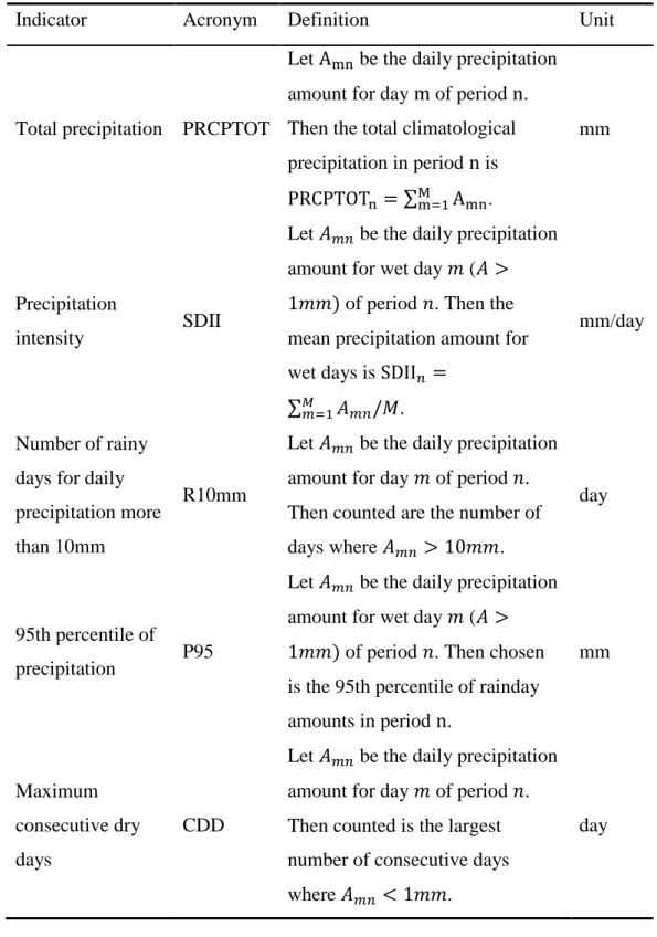
In order to measure the climate characteristics of simulated precipitations, five indices including precipitation means and extremes are used (Jiang et al., 2012). They are all calculated with the diagnostic software provided by the Statistical and Regional Dynamical Downscaling of Extremes for European Regions (STARDEX) (Haylock et

al., 2006). Their definition is presented in Table 1.

Performance metrics include a parameter assessing the distribution of daily precipitations, skill Score ( _`)a0b), and the Taylor diagram describing the spatial pattern of a geophysical variable (Perkins et al., 2007; Liu et al., 2011; Fu et al., 2013b; Taylor,

2001).

`)a0b was proposed in Perkins et al. (2007) to measure the coincidence of two PDF curves by calculating the cumulative minimum value of the two distributions.

`)a0b= ∑ c3d3efe(g# h, a) (7)

Where h and a are the modelled and observed 3th probability values of each bins and

i is the number of bins. It varies from 0 (no overlapping at all) to 1 (total matching between the two distributions).

Taylor Diagram (Taylor, 2001) provides a statistical summary of patterns similarity between simulations and observations in terms of spatial correlation coefficient, centered root-mean-square (RMS) difference, and ratio of spatial standard deviations. A perfect simulation would have the value of 1 for the centered pattern root mean square error (RMSE), and 0 for the spatial correlation. The ratio of spatial standard deviations would be 1.

2.4 Time windows for 1.5

℃

and 2

℃

global warming targets

As defined in the Paris climate Agreement, the 1.5℃ and 2℃ global warming thresholds are relative to the pre-industrial level. The period 1861-1900 is selected as a common pre-industrial period in this study. The emission scenario is RCP4.5. Time

(13)

series of global averaged temperature anomalies are firstly smoothed by a 21-year moving average before selecting the year for which the 1.5℃ or 2℃ threshold is firstly reached. Finally a period of 21 years in total is defined with 10 years before and after the nominative year, as shown in Table 2. This way of defining the time windows is consistent and comparable with a few recent studies, e.g., Hu et al (2017) and Shi et al

(2017), on China’s regional climate change corresponding to 1.5°C and 2°C warming

levels. We need to point out that the climate reference period is from 1986 to 2005, defined as present-day climate, although the 1.5℃ and 2℃ warming targets are relative to the pre-industrial. The global mean surface air temperature increases by 0.9°C from pre-industrial to present-day in the ensemble mean of our three GCMs. The net warming for the cases of 1.5°C and 2°C warming levels would be of 0.6℃ and 1.1℃ respectively.

3 Climate properties of extreme precipitations in GCMs and NHMM

In our previous study, we used ERA-40 large-scale circulation from 1991 to 2002 in the construction and calibration of NHMM to stochastically simulate summer (1 June to 31 August) daily precipitations in Eastern China. NHMM showed a very good skill in simulating the probability distribution of precipitations, their spatial distribution patterns and their interannual variability (Ding et al., 2016). In this paper, we will further evaluate the performance of NHMM, but in the context of its application to outputs of three GCMs. We put emphasis on the added value of NHMM compared to the performance of original GCMs. Since this evaluation is done for present-day climate, it also provides a reference for projecting future extreme rainfall changes.

(14)

To assess the ability of NHMM and that of the three driving GCMs, we first show the Quantile-Quantile plots performed on daily precipitation for four major stations in the region. As shown in Fig. 2, there is a systematic bias in the distribution of daily precipitations in GCMs. For any quantile, the simulated rainfall amount is significantly lower than the observed one. The largest difference is above 60mm (Fig. 2a and Fig. 2c). After downscaling with NHMM, models are rather close to observation with an absolute error smaller than 20mm. It indicates that NHMM indeed improves the statistical behaviors of daily precipitation. For daily precipitation rate below 50mm, NHMM is highly consistent with observation at Nanjing and Wuhan. Similarly, NHMM does a good job for daily rainfall rate below 40mm at Hangzhou and Hefei. For heavy rain greater than 50mm, the simulation by NHMM at Nanjing, Hangzhou and Hefei is generally smaller than observation, while at Wuhan and for precipitation greater than 80mm, the simulation is larger than observation.

In terms of differences among models, the ability of simulation below 70mm in MPI-ESM-MR gets closer to observation than other two models and the multi-model ensemble, while for daily rainfall greater than 70mm, BCC-CSM1.1(m) is slightly better than other models. The simulation capability of the multi-model ensemble generally keeps at middle level among the three models. After downscaling with NHMM, the outputs of all the three models and the multi-model ensemble tend to coincide. We almost cannot distinguish them from each other in Fig. 2.

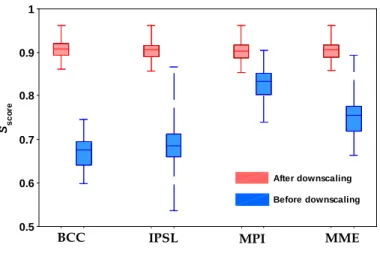
We now examine all the stations in the region. Fig. 3 gives box-and-whisker plots showing the distributions of _`)a0b at the 56 stations. When _`)a0bare closer to 1, the simulated distribution for all stations is closer to the observed one. It is clear that NHMM improves significantly the ability of all the three models and the multi-model ensemble in simulating the distribution of daily precipitation. Detailed results show that

(15)

the medians of _`)a0b for BCC-CSM1.1(m), IPSL-CM5A-MR, MPI-ESM-MR and multi-model ensemble are 0.68, 0.68, 0.83 and 0.75, respectively. After downscaling with NHMM, the medians of _`)a0b increase to 0.91, 0.90, 0.90, and 0.91, respectively. In general, the _`)a0b for each station almost is above 0.85, in which the largest _`)a0b is up to 0.96. The ranges of _`)a0b are significantly decreased among different stations.

If we examine individual models and the multi-model ensemble, MPI-ESM-MR gives the best results on _`)a0b, while BCC-CSM1.1(m) and IPSL-CM5A-MR show the largest improvement after NHMM downscaling with the medians of S_jklmn increasing to more than 0.9 (Fig. 3).

3.2 Spatial distribution of precipitation indices

In this section we turn our attention to the performance reproducing the spatial pattern by NHMM along with the mean and extreme precipitation indices. Fig. 4 shows the Taylor diagram for the five precipitation indices in the three global models and the multi-model ensemble to comprehensively evaluate the spatial distribution. The same is shown for results with the application of NHMM. There is generally a weak ability in GCMs. Specifically, the spatial correlation coefficients of major indices between the simulations and observations are less than 0.4 and the maximum does not exceed 0.6; the standard deviations are relatively scattered; the RMSEs are generally greater than 0.75. After downscaling, NHMM improves significantly the spatial distribution of precipitation indices. Except CDD that does not show improvement with NHMM, other precipitation indices observe their spatial correlation coefficients increasing to more than 0.8; the standard deviations remain between 0.9 and 1.3; the RMSEs decrease to less than 0.75. Among the different indices measuring spatial patterns of precipitation, there is a greater improvement in simulating PRCPTOT and R10mm with spatial correlation coefficients larger than 0.9 and RMSEs smaller than 0.5. Again, CDD shows

(16)

its weakest score compared to other indices. The first-order Markov chain, obviously, cannot well capture this persistent behavior of weather sequences. Burger et al. (2012), by comparing different statistical downscaling methods, also conclude that most of them fail to reproduce CDD.

To sum up, NHMM effectively enhances the ability of models in simulating summer daily precipitation and spatial distribution over the Yangtze-Huaihe River Basin. It provides a basis for projecting future change of daily precipitation under warmer climate using this method. After downscaling, the PDF curves of the simulations get closer to the observations. The median of skill score for BCC-CSM1.1(m), IPSL-CM5A-MR, MPI-ESM-MR and multi-model ensemble is increased by 0.23, 0.22, 0.07 and 0.16, respectively. The ranges of the _`)a0b are significantly decreased among different stations. The spatial correlation coefficients of PRCPTOT, SDII, R10mm and P95 are improved from less than 0.6 to more than 0.8, and the root mean square errors of the above four are generally decreased to 0.75 or less, in which PRCPTOT and R10mm have the optimal improvement.

4 Future projections

In view of the added value of NHMM compared to performance of initial GCMs, we apply the established NHMM to further project future change in daily precipitation or extreme precipitation during 2017-2036, 2046-2065 and 2080-2100 under the RCP4.5 emission scenario, as well as the global warming period of 1.5℃ and 2℃.

4.1 Change in daily precipitation distribution

We can now calculate the probability distribution functions of daily precipitations with different intensities from all the 56 stations in our region. This is repeated for present-day and the three future periods respectively. Instead of making visual

(17)

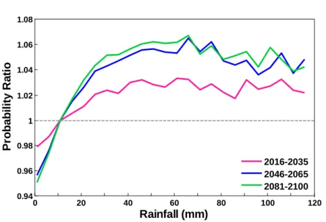
inspection among the four curves (not shown), we can quantify the variations from present-day to future horizons by calculating the ratio of probabilities for each bin of intensities. This concept is close to the probability ratio (PR) introduced and used by

Stott et al. (2004) and Fischer et al. (2015) to measure the risk variation. Fig. 5 shows

PR of daily precipitation distribution, calculated for the whole domain with data from the multi-model ensemble for three periods of the 21st century, 2017–2036, 2046–2065 and 2080–2100. Generally speaking, PR of light rain (0.1-9.9mm) shows a decreasing trend, while that of strong rainfalls (larger than 9.9mm per day) increases. The rate of PR seems to slow down when the time goes on (a saturation effect). Specifically, for light rain (0.1-9.9mm/day), PR in average during 2017–2036, 2046–2065 and 2080– 2100 is 0.983, 0.966 and 0.962, respectively, relative to 1986-2005. For moderate rain (10-24.9mm/day), the occurrence probabilities increase by a factor of 1.005, 1.014 and 1.016, respectively. For heavy rain (25-49.9mm/day), the occurrence probabilities increase by a factor of 1.026, 1.047 and 1.053, respectively. For the rainstorm (50-99.9mm), the occurrence probabilities increase by a factor of 1.027, 1.052 and 1.055, respectively. For heavy rainstorm (more than 99.9mm), the occurrence probabilities increase by a factor of 1.026, 1.045 and 1.047, respectively. In general, summer daily precipitation in the middle and low reach of the Yangtze River has a higher occurrence probability for strong rainfalls (> 10 mm/day) and a weaker probability for light rainfalls (< 10 mm/day).

4.2 Change in geographic distribution of precipitation indices

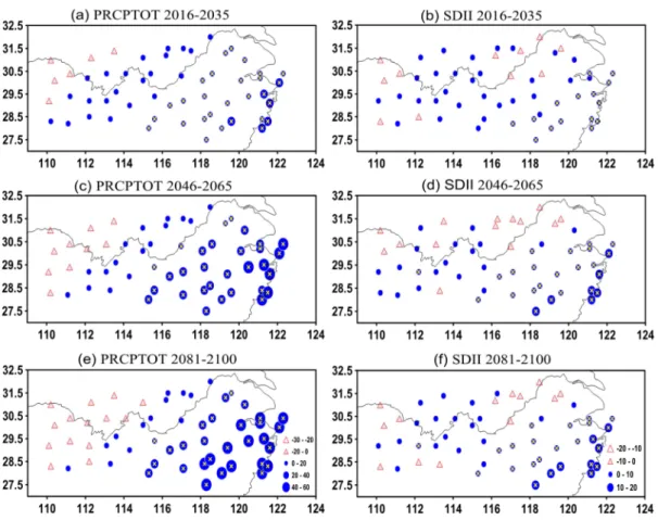
The spatial distribution of PRCPTOT and SDII changes for 2017–2036, 2046– 2065 and 2080–2100, relative to 1986-2005, is shown in Fig. 6. In the early 21st century, both PRCPTOT and SDII increase at major stations in the east, with relative changes keeping below 20% and 10%, respectively, while the two indices decrease in the west.

(18)

In the middle 21st century, larger variations appear for the two indices, compared to the former period. For example, PRCPTOT across the coastal area increases by 40%. In the late 21st century, PRCPTOT and SDII show more dry areas for stations in the west, while the difference between the west and the east tends to amplify. It’s noted that the increase of PRCPTOT is generally stronger than that in SDII.

Fig. 7 shows relative changes of extreme precipitation indices R10mm, P95 and

CDD. The trend of R10mm is similar to that of P95, but opposite to that of CDD. In the early 21st century, R10mm and P95 at major stations increase with the relative changes keeping below 20% and 10%, respectively, while CDD generally decreases. In the middle 21st century, larger variations appear in the three indices and at more stations in the east. R10mm and P95 increase by more than 20% and 10%, and CDD decreases by over 20%. In the late 21st century, the increase of R10mm across the eastern region is up to over 40% and the decrease of CDD keeps more than 20%, while CDD over the western area decreases by less than 20%. To sum up, extreme and local characteristic of future summer rainfall over the Yangtze-Huaihe River Basin will show a gradual increase with smaller increase (or even weak decrease) in western region and larger increase in eastern region.

4.3 Response of extreme precipitation under the global warming of 1.5

℃

and 2

℃

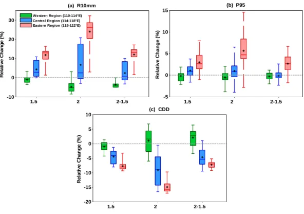
Considering important economic and geopolitical issues in relation to the global warming levels of 1.5℃ and 2.0℃ in the Paris Agreement, we put particular attention to responses of extreme precipitation in our region of investigation under the two warming targets. Precipitation indices in terms of geographic distributions are quite similar to what is shown in Fig. 7, R10mm, P95 and CDD have a spatially coherent change with wetter trend in eastern region and drier trend in western region under 1.5℃ warming target, while these trends are more significant under 2℃ target. Considering the fact that

(19)

there is a general gradient from west to east in our region of investigation, we divided the 56 stations into three groups (west, middle and east) with roughly equal number of stations. Statistics for each group are given in Fig. 8 in the form of box-whisker plots. For both R10mm and P95, there is a slight decrease in the west, but there are increases in the middle and east. Changes in 2°C are generally amplified compared to those in 1.5°C warming. The additional half-degree warming from 1.5℃ to 2℃ implies changes of -3.7% (-0.3%), 2.4% (-0.1%) and 12.1% (2.7%) for R10mm (P95) and for the west, middle and east respectively. For CDD, we observe a reverse gradient from west to east. The additional half-degree warming induces an increase of 2.1% in the west, but decreases of -4.6% and -7.2% in other two regions.

5 Summary and discussion

A statistical climate downscaling based on NHMM was constructed and used to simulate summer daily precipitation in Central and Eastern China. The nonhomogeneous term was the large-scale atmospheric circulation from three global climate models, i.e., BCC-CSM1.1(m), IPSL-CM5A-MR and MPI-ESM-MR. NHMM became thus a powerful tool to perform relevant climate downscaling, including future projection of summer daily rainfall under the RCP4.5 emission scenario. Main conclusions are the following.

(1) NHMM effectively enhances the ability of global climate models in simulating summer daily rainfall in the middle and low reach of the Yangtze River in Eastern China. Absolute errors of daily precipitation distribution shown in Quantile-Quantile plots are largely reduced, from about 60mm in global models to generally below 20mm in NHMM downscaling. The improvement is also confirmed with quantitative measures, the skill score. Spatial correlation coefficients of PRCPTOT, SDII, R10mm and P95 are

(20)

improved from less than 0.6 to more than 0.8. The RMSEs of the above four indices are generally decreased to 0.75 or less. CDD shows little improvement in NHMM, due to certainly inadequacy of the first-order Markov chain for long-lasting phenomenon.

(2) Future rainfall changes are projected based on NHMM for three future periods, 2017–2036, 2046–2065 and 2080–2100, under the RCP4.5 scenario. Our study area exhibits a general wetter trend in the future, but a different repartition in rainfall distribution. Daily precipitation smaller than 10mm would decrease and that above 10mm would increase, in which the largest risk in rainstorm (50-99.9mm/day) increases by a factor of 1.027~1.055. The changing rate keeps significant until the middle of the 21st century, and presents a saturation effect in the late 21st century. In addition, PRCPTOT, SDII, R10mm and P95 have a gradually increasing trend during early, middle and late 21st century, while CDD is relatively decreasing with flood in eastern region and drought in western region. There are obvious changes occurring in eastern region (118-122°E) with 95% significance level, and PRCPTOT or R10mm increases by 40%~60% in the late 21st century. Conversely, CDD decreases by -30%~ -20% there. Rainfall changes presented in this work are confirmed to be coherent with changes in atmospheric general circulation. Results, not shown in this paper, will be reported in the future.

(3) Under the global warming of 1.5℃ and 2℃, the response characteristics of extreme precipitation for all stations in Eastern China show that R10mm, P95 and CDD have a spatially coherent change with wetter trend in eastern region and drier trend in western region under 1.5 ℃ warming target, while these trends would be more pronounced at 2℃ target. From 1.5℃ to 2℃ target, the additional half-degree warming makes R10mm (P95) to vary by -3.7% (-0.3%), 2.4% (-0.1%) and 12.1% (2.7%) in western, central and eastern regions, respectively. Conversely, CDD varies by 2.1%,

(21)

-Accepted manuscript. Guo et al. 2018 International J. of Climatology https://doi.org/10.1002/joc.5882 page 20

4.6% and -7.2%, respectively. It’s noted that the 1.5℃ and 2℃ warming targets relative to pre-industrial period imply a warming of 0.6℃ and 1.1℃ relative to present-day period for MME, respectively.

Our results provide a relevant reference for statistical downscaling of daily rainfall in Eastern China with a nonhomogeneous hidden Markov chain. However, it is necessary to point out that rainfalls are often greatly affected by topography, and mesoscale and small scale systems, which creates intrinsic uncertainties for climate projection. There are also uncertainties in relation to future emission scenarios and to GCMs themselves. To reduce uncertainties of climate downscaling and projection, multiple models and multiple approaches need to be further promoted. Finally, in terms of NHMM improvement, we need to study model sensitivity in function of tunable parameters or to compare it with other statistical theories and approaches, already used in the East Asian monsoon region.

Acknowledgments. We thank the editor and anonymous reviewers for their

constructive comments. We acknowledge the PCMDI for collecting and archiving the CMIP5 model output and the World Climate Research Programme’s Working Group on Coupled Modelling. This study was jointly supported by the National Key Research and Development Program of China (2017YFA0603804, 2016YFA0600402) and the State Key Program of National Natural Science Foundation of China (41230528).

Reference

Bates BC, Charles SP, Hughes JP. 1998. Stochastic downscaling of numerical climate model simulations. Environ. Modell. Softw. 13: 325-331, doi:

(22)

10.1016/S1364-Accepted manuscript. Guo et al. 2018 International J. of Climatology https://doi.org/10.1002/joc.5882 page 21

8152(98)00037-1.

Ben Alaya MA, Chebana F, Ouarda TBMJ. 2015. Probabilistic Multisite Statistical Downscaling for Daily Precipitation Using a Bernoulli-Generalized Pareto Multivariate Autoregressive Model. J. Clim. 28: 2349-2364, doi:

10.1175/JCLI-D-14-00237.1.

Brier GW. 1950. Verification of forecasts expressed in terms of probability. Mon. Wea.

Rev. 78: 1-3, doi: 10.1175/1520-0493(1950)078<0001:VOFEIT>2.0.CO;2.

Bürger G, Murdock TQ, Werner AT, Sobie SR, and Cannon AJ. 2011. Downscaling extremes: An intercomparison of multiple statistical methods for present climate. J.

Clim. 25: 4366–4388, doi: 10.1175/JCLI-D-12-00249.1.

Charles SP, Bates BC, Hughes JP. 1999. A spatiotemporal model for downscaling precipitation occurrence and amounts. J. Geophys. Res. 104(D24): 31657-31669, doi: 10.1029/1999JD900119.

Cioffi F, Conticello F, Lall U, Marotta L, Telesca V. 2016. Large scale climate and rainfall seasonality in a Mediterranean Area: Insights from a nonhomogeneous Markov model applied to the Agro-Pontino plain. Hydrol. Processes 1-9, doi:

10.1002/hyp.110 61.

Dayon G, Boé J, Martin E. 2015. Transferability in the future climate of a statistical downscaling method for precipitation in France. J. Geophys. Res. 120(3):1023-1043, doi: 10.1002/2014JD022236.

Dempster AP, Laird NM, Rubin DB. 1977. Maximum likelihood from incomplete data via EM algorithm. J. Royal Statistical Society Series B-Methodological 39(1): 1– 38.

Ding M, Jiang ZH, Chen WL. 2016. Simulation and evaluation of summer daily precipitation based on nonhomogeneous hidden Markov model over the

(23)

Yangtze-Accepted manuscript. Guo et al. 2018 International J. of Climatology https://doi.org/10.1002/joc.5882 page 22

Huaihe River Basin. J. Meteor. Res. 74(5): 757-771. (in Chinese)

Fischer EM, Knutti R. 2015. Anthropogenic contribution to global occurrence of heavy-precipitation and high-temperature extremes. Nat. Clim. Change 5: 560-564, doi:

10.1038/nclimate2617.

Fu GB, Charles SP, Kirshner S. 2013a. Daily rainfall projections from general circulation models with a downscaling nonhomogeneous hidden Markov model (NHMM) for south-eastern Australia. Hydrol. Processes 27(25): 3663–3673, doi:

10.1002/hyp.9483.

Fu GB, Liu ZF, Charles SP, et al. 2013b. A score-based method for assessing rhe performance of GCMs: A case study of south-eastern Australia. J. Geophys. Res.

118(10): 4154-4167, doi: 10.1002/jgrd.50269.

Greene AM, Robertson AW, Smyth P, Triglia S. 2011. Downscaling projections of Indian monsoon rainfall using a non-homogeneous hidden Markov model. Quart. J.

Roy. Meteor. Soc. 137: 347-359, doi: 10.1002/qj.788.

Haylock MR, Cawley GC, Harpham C, et al. 2006. Downscaling heavy precipitation over the United Kingdom: a comparison of dynamical and statistical methods and their future scenarios. Int. J. Climatol. 26(10):1397-1415, doi: 10.1002/joc.1318. Hu T, Sun Y, Zhang XB. 2017. Temperature and precipitation projection at 1.5℃ and

2.0℃ increase in global mean temperature. Chinese Sci. Bull. 62(26): 3098-3111. (in Chinese)

Hughes JP, Guttorp P. 1994. A class of stochastic models for relating synoptic atmospheric patterns to regional hydrologic phenomena. Water Resour. Res. 30(5): 1535-1546, doi: 10.1029/93WR02983.

Hughes JP, Guttorp P, Charles SP. 1999. A non-homogeneous hidden Markov model for precipitation occurrence. J. Roy. Stat. Soc. 48C: 15–30.

(24)

Hundecha Y, Sunyer MA, Lawrence D, et al. 2016. Inter-comparison of statistical downscaling methods for projection of extreme flow indices across Europe. J.

Hydrol. 541(6):1273-1286, doi: 10.1016/j.jhydrol.2016.08.033.

Jha SK, Mariethoz G, Evans J, et al. 2015. A space and time scale-dependent nonlinear geostatistical approach for downscaling daily precipitation and temperature. Water

Resour. Res. 51(8):6244-6261, doi: 10.1002/2014WR016729.

Jiang DB, Zhang Y and Sun YQ. 2009. Ensemble projection of 1-3℃ warming in China.

Chin. Sci. Bull. 54: 3326-3334, doi: 10.1007/s11434-009-0313-1.

Jiang ZH, Li W, Xu JJ, Laurent Li. 2015. Extreme Precipitation Indices over China in CMIP5 models. Part 1: Models evaluation. J. Clim. 28: 8603-8619, doi:

10.1175/JCLI-D-15-0099.1.

Jiang ZH, Song J, Li L, et al. 2012. Extreme climate events in China: IPCC-AR4 model evaluation and projection. Climatic Change 110(1-2): 385-401, doi:

10.1007/s10584-011-0090-0.

Jones PD, Harpham C, Burton A, Goodess CM. 2016. Downscaling regional climate model outputs for the Caribbean using a weather generator. Int. J. Climatol. doi:

10.1002/joc.4624.

Kirshner S. 2005. Modeling of multivariate time series using hidden Markov models. University of California, Irvine.

Knutti R, Rogelj J, Sedlacek J, Fischer EM. 2016. A scientific critique of the two-degree climate change target. Nat. Geosci. 9(1): 13-18, doi: 10.1038/NGEO2595.

Li W, Jiang ZH, Xu JJ, Laurent Li. 2016. Extreme Precipitation Indices over China in CMIP5 Models. Part II: Probabilistic Projection. J. Clim. 29(24): 8989-9004, doi:

10.1175/JCLI-D-16-0377.1.

(25)

China from 1.5 ℃ to 2.0 ℃ global warming levels. Sci. Bull. doi:

10.1016/j.scib.2017.12.021.

Liu ZF, Xu ZX, Charles SP, et al. 2011. Evaluation of two statistical downscaling models for daily precipitation over an arid basin in China. Int. J. Climatol. 31(13): 2006-2020, doi: 10.1002/joc.2211.

Perkins SE, Pitman AJ, Holbrook NJ, Mcaneney J. 2007. Evaluation of the AR4 climate models’ simulated daily maximum temperature, minimum temperature, and precipitation over Australia using probability density functions. J. Clim. 20: 4356-4376, doi: 10.1175/JCLI4253.1.

Rabiner LR, Juang BH. 1986. An introduction to hidden Markov models. IEEE ASSP Magazine 3(1): 4-11.

Robertson AW, Kirshner S, Smyth P. 2003. Hidden Markov models for modeling daily rainfall occurrence over Brazil. University of California, 23.

Robertson AW, Kirshner S, Smyth P. 2004. Downscaling of daily rainfall occurrence over northeast Brazil using a hidden Markov model. J. Clim. 17(22): 4407-4424, doi: 10.1175/JCLI-3216.1.

Schaeffer M, Hare W, Rahmstorf S, Vermeer M. 2012. Long-term sea-level rise implied by 1.5 ℃ and 2 ℃ warming levels. Nat. Clim. Change 2: 867-870, doi:

10.1038/nclimate1584.

Shi C, Jiang ZH, Chen WL. 2017. Changes in temperature extremes over China under 1.5 ℃ and 2 ℃ global warming targets. Adv. Clim. Change Res. doi:

10.1016/j.accre.2017.11.003 .

Stott PA, Stone DA, Allen MR. 2004. Human contribution to the European heatwave of 2003. Nature 432: 610-614, doi: 10.1038/nature03089.

(26)

rainfall amount in peninsular malaysia. Jurnal Teknologi (Sciences & Engineering)

63(2): 75-80, doi: 10.11113/jt.v63.1916.

UNFCC. Adoption of the Paris Agreement. 2015. Report No. FCCC/CP/2015/L.9/Rev.1.

http://unfccc.int/resource/docs/2015/cop21/eng/l09r01.pdf.

Taylor KE. 2001. Summarizing multiple aspects of model performance in a single diagram. J. Geophys. Res. 106(D7): 7183-7192, doi: 10.1029/2000JD900719. Wu D, Jiang ZH, Ma TT. 2016. Projection of summer precipitation over the

Yangtze-Huaihe River basin using multimodel statistical downscaling based on canonical correlation analysis. J. Meteor. Res. 30(6): 867-880, doi:

10.1007/s13351-016-6030-1.

Xu CH, Luo Y, Xu Y. 2011. Projected changes of precipitation extremes in river basins over China. Quat. Int. 244: 149-158, doi: 10.1016/j.quaint.2011.01.002.

Yang H, Jiang ZH, Li L. 2016. Biases and Improvements in three Dynamical Downscaling Climate Simulations over China. Climate Dyn. 47(9-10): 3235-3251, doi: 10.1007/s00382-016-3023-9.

(27)

Table 1. Indicator, acronym, definition and unit of five indices used in this study

Indicator Acronym Definition Unit

Total precipitation PRCPTOT

Let A_pq be the daily precipitation amount for day m of period n. Then the total climatological precipitation in period n is

PRCPTOTq = ∑vp# Apq.

mm

Precipitation

intensity SDII

Let w_hx be the daily precipitation amount for wet day e (w > 1ee) of period d. Then the

mean precipitation amount for wet days is SDII_x =

∑{h# whx/c.

mm/day

Number of rainy days for daily precipitation more than 10mm

R10mm

Let whx be the daily precipitation

amount for day e of period d.

Then counted are the number of days where w_hx > 10ee.

day

95th percentile of

precipitation P95

amount for wet day e (w > 1ee) of period d. Then chosen

is the 95th percentile of rainday amounts in period n. mm Maximum consecutive dry days CDD

amount for day e of period d.

Then counted is the largest number of consecutive days where w_hx < 1ee.

(28)

Table 2 Time windows in the three global models when global warming levels at 1.5℃ and 2℃are satisfied, relative to pre-industrial period.

Model 1.5℃ warming year 2℃ warming year

BCC-CSM1-1(m) 2014 (2004, 2024) 2039 (2029, 2049)

IPSL-CM5A-MR 2017 (2007, 2027) 2034 (2024, 2044)

(29)

Fig. 1. Schematic of NHMM and its progressing in time. …… …… …… …… …… …… R_T-1 R_T R_t R₂ R₁ S₁ S₂ X₁ X₂ S_t X_t S_T-1 S_T X_T-1 X_T

(30)

Fig. 2. Quantile-Quantile plots of simulated daily precipitations in GCMs (before downscaling) and NHMMs (after downscaling), and observed precipitations at four operational stations: Nanjing (a), Hangzhou (b), Wuhan (c) and Hefei (d). N-B (yellow circle), N-I (green circle), and N-M (red circle) denote outputs from NHMM simulations driven by three GCMs: BCC-CSM1.1(m) (orange triangle), IPSL-CM5A-MR (green triangle), MPI-ESM-IPSL-CM5A-MR (red triangle). MME denotes multi-model ensemble (blue triangle) from the three GCMs, and N-MME the multi-model ensemble (blue circle) after downscaling, respectively.

0 30 60 90 120 0 30 60 90 120 Observed (mm) M o d e ll e d ( m m ) (a) Nanjing N-MME Ss=0.9188 MME Ss=0.7542 0 30 60 90 120 0 30 60 90 120 Observed (mm) M o d e ll e d ( m m ) (c) Wuhan N-MME Ss=0.8696 MME Ss=0.7077 0 30 60 90 120 0 30 60 90 120 Observed (mm) M o d e ll e d ( m m ) (d) Hefei N-MME Ss=0.9078 MME Ss=0.7754 0 30 60 90 120 0 30 60 90 120 Observed (mm) M o d e ll e d ( m m ) (b) Hangzhou N-B BCC-CSM1.1(m) N-I IPSL-CM5A-MR N-M MPI-ESM-MR N-MME MME N-MME Ss=0.9047 MME Ss=0.7649

(31)

Fig. 3. Box-and-whisker plot showing the distribution of _`)a0b at 56 stations before (blue, i.e. in GCMs) and after (red) NHMM downscaling.

Fig. 4. Taylor Diagram showing five precipitation indices (PRCPTOT, SDII, R10mm, P95 and CDD) in three global climate models (BCC, IPSL, MPI) and their multi-model

0.5 0.6 0.7 0.8 0.9 1 Ss c o re

BCC IPSL MPI MME

After downscaling Before downscaling

(32)

ensemble (MME) (in hollow symbols). Corresponding results from NHMM downscaling are shown in solid symbols.

Fig. 5. Probability density function normalized by that of the reference climate from 1986 to 2005 for summer daily precipitation in the middle and low reaches of the Yangtze River and for all NHMM simulations with three GCMs from 2016 to 2035, from 2046 to 2065 and from 2081 to 2100, respectively. To calculate the PR, we firstly divide the daily precipitation (>0.1mm) into several intervals of 5mm; furthermore, a ratio of the occurrence frequency in future period to that in reference period for each interval is the PR value.

0 20 40 60 80 100 120 0.94 0.96 0.98 1 1.02 1.04 1.06 1.08 Rainfall (mm) P ro b a b il it y R a ti o 2016-2035 2046-2065 2081-2100

(33)

Fig. 6. Relative changes of PRCPTOT (a, c, e) and SDII (b, d, f) during 2017–2036, 2046–2065 and 2080–2100, relative to 1986-2005 (unit: %). Yellow cross represents the station that passes the 95% significance student’s t test.

(34)

(35)

Fig. 8. Boxplots showing the distribution of relative changes (in %) of R10mm (a), P95 (b) and CDD (c) in the three sub-regions, western (green, 110-114°E), central (blue, 114-118°E) and eastern (red, 118-122°E), under the global warming of 1.5℃, 2℃ and half-degree warming from 1.5 to 2℃. The upper and lower limits of box indicate the 75th and 25th percentiles among stations; the horizontal line (the black asterisk) inside box indicates multi-station ensemble median (mean); and the whiskers show the range among stations. 1.5 2 2-1.5 -5 0 5 10 15 R e la ti v e C h a n g e ( % ) (b) P95 1.5 2 2-1.5 -20 -15 -10 -5 0 5 10 R e la ti v e C h a n g e ( % ) (c) CDD 1.5 2 2-1.5 -10 0 10 20 30 R e la ti v e C h a n g e ( % ) (a) R10mm

Western Region (110-114°E) Central Region (114-118°E) Eastern Region (118-122°E)