HAL Id: lirmm-00818393
https://hal-lirmm.ccsd.cnrs.fr/lirmm-00818393
Submitted on 26 Apr 2013
HAL is a multi-disciplinary open access
archive for the deposit and dissemination of
sci-entific research documents, whether they are
pub-lished or not. The documents may come from
teaching and research institutions in France or
abroad, or from public or private research centers.
L’archive ouverte pluridisciplinaire HAL, est
destinée au dépôt et à la diffusion de documents
scientifiques de niveau recherche, publiés ou non,
émanant des établissements d’enseignement et de
recherche français ou étrangers, des laboratoires
publics ou privés.
Adaptively Synchronous Scalable Spread Spectrum
(A4S) Data-Hiding Strategy for Three-Dimensional
Visualization
Khizar Hayat, William Puech, Gilles Gesquière
To cite this version:
Khizar Hayat, William Puech, Gilles Gesquière. Adaptively Synchronous Scalable Spread Spectrum
(A4S) Data-Hiding Strategy for Three-Dimensional Visualization. Journal of Electronic Imaging,
SPIE and IS&T, 2010, 19 (2), pp.023011-1–023011-1. �lirmm-00818393�
Adaptively synchronous scalable spread spectrum (A4S)
data-hiding strategy for three-dimensional visualization
Khizar Hayat
COMSATS Institute of Information Technology Department of Computer Science
University Road Abbottabad, Pakistan William Puech University of Montpellier II LIRMM Laboratory UMR 5506 CNRS 161, Rue Ada 34392 Montpellier Cedex 05 France [email protected] Gilles Gesquière Aix-Marseille University LSIS UMR CNRS 6168 IUT, Rue R. Follereau
13200 Arles, France
Abstract. We propose an adaptively synchronous scalable spread spectrum (A4S) data-hiding strategy to integrate disparate data, needed for a typical 3-D visualization, into a single JPEG2000 for-mat file. JPEG2000 encoding provides a standard forfor-mat on one hand and the needed multiresolution for scalability on the other. The method has the potential of being imperceptible and robust at the same time. While the spread spectrum (SS) methods are known for the high robustness they offer, our data-hiding strategy is removable at the same time, which ensures highest possible visualization qual-ity. The SS embedding of the discrete wavelet transform (DWT)-domain depth map is carried out in transform (DWT)-domain YCrCb com-ponents from the JPEG2000 coding stream just after the DWT stage. To maintain synchronization, the embedding is carried out while taking into account the correspondence of subbands. Since security is not the immediate concern, we are at liberty with the strength of embedding. This permits us to increase the robustness and bring the reversibility of our method. To estimate the maximum tolerable error in the depth map according to a given viewpoint, a human visual system (HVS)-based psychovisual analysis is also presented.© 2010 SPIE and IS&T. 关DOI: 10.1117/1.3427159兴
1 Introduction
The first decade of the twenty-first century has witnessed a revolution in the form of memory and network speeds and computing efficiencies. Simultaneously, the platform and
client diversity base have also been expanding, with pow-erful workstations on one extreme and handheld portable devices, like smart phones, on the other. Still versatile are the clients whose needs evolve with every passing moment. Hence, the technological revolution notwithstanding, deal-ing with the accompanydeal-ing diversity is always a serious challenge. This challenge is more glaring in the case of applications where huge data are involved. One such appli-cation is the area of 3-D visualization where the problem is exacerbated by the involvement of more than one set of data.
A typical 3-D visualization is based on at least two sets of data: a 2-D intensity image, called texture, with a corre-sponding 3-D shape rendered in the form of a range image, a shaded 3-D model, and a mesh of points. A range image, also sometimes called a depth image, is an image in which the pixel value reflects the distance from the sensor to the imaged surface.1 The underlying terminology may vary from field to field, e.g., in terrain visualization height/depth data are represented in the form of discrete altitudes which, upon triangulation, produce what is called a digital eleva-tion model 共DEM兲: the texture is a corresponding aerial photograph overlaid onto the DEM for visualization. Simi-larly, in 3-D facial visualization, the D color face image represents the texture but the corresponding depth map is usually in the form of what is called a 2.5-D image. The
Paper 09119RR received Jul. 10, 2009; revised manuscript received Mar. 22, 2010; accepted for publication Mar. 26, 2010; published online May 21, 2010.
latter is usually obtained2 by the projection of the 3-D po-lygonal mesh model onto the image plane after its normal-ization.
To cater to client diversity and unify the disparate 3-D visualization data, we are proposing in this work an adap-tively synchronous scalable spread spectrum 共A4S兲 data-hiding strategy. We are relying on the multiresolution char-acter of the DWT-based JPEG2000 format for scalability, whereas data hiding is being employed to unify the data into a single standard JPEG2000 format file. The proposed data-hiding method is blind, robust, and imperceptible. Ro-bustness is offered by spread spectrum 共SS兲 embedding, and imperceptibility is provided by the removable nature of the method.
One might wonder why we employ data hiding when a depth map can be easily inserted to the format header of JPEG2000 compressed texture. One can even think of con-sidering the DEM data as the fourth component besides the YCrCb components of texture. Our counterargument is that although there exist such approaches, e.g., GeoJP23 and GMLJP24for terrain visualization, the problem is the esca-lation in the size of the texture file. That is to say, the process is additive and the final coded texture is of the order X + Y, where X is the size of the original texture and Y is the size of its depth map. What we are after is that the coded texture should be on the order of X, i.e., X + Y⬇X. In addition, the data will be synchronized and each texture block/coefficient would roughly contain its own depth map coefficient, a feature lacking in the aforementioned ap-proaches, and they may need explicit georeferencing to achieve it. Note that GeoJP2 is a GeoTIFF-inspired method for adding geospatial metadata to a JPEG2000 file. The GeoTIFF specification5defines a set of TIFF tags provided to describe all cartographic information associated with TIFF imagery that originates from satellite imaging sys-tems, scanned aerial photography, scanned maps, and DEM. In itself, GeoTIFF does not intend to become a re-placement for existing geographic data interchange stan-dards. The mechanism is simple using the widely supported GeoTIFF implementations, but the introduction of new uni-versally unique identification共UUID兲 boxes has the disad-vantage that there is an increase in the original JPEG2000 file size. GMLJP2, on the other hand, envisages the use of the geography markup language 共GML兲 within the XML boxes of the JPEG 2000 data format in the context of geo-graphic imagery. A minimally required GML definition is specified for georeferencing images while also giving guidelines for encoding of metadata, features, annotations, styles, coordinate reference systems, and units of measure as well as packaging mechanisms for both single and mul-tiple geographic images. DEMs are treated the same way as other image use cases, whereas coordinate reference system definitions are employed using a dictionary file. Thus DEM is either provided as a TIFF file and its name is inserted between proper GML tags, or its points are directly inserted into the GMLJP2 file. In the former case, there is no reduc-tion in the number of files, whereas in the latter case the amount of data is increased.
In real-time face visualization context, two areas are of special interest in contemporary research, namely video conference and video surveillance. In earlier video confer-ence applications, the aim was to change the viewpoint of
the speaker. This allowed in particular the recreation of a simulation replica of a real meeting room by visualizing virtual heads around a table.6 Despite the fact that many technological barriers have been eliminated—thanks to the availability of cheap cameras, powerful graphic cards, and high bitrate networks—there is still no efficient product that offers a true conferencing environment. Some companies, such as Tixeo in Montpellier, France7propose a 3-D envi-ronment where interlocutors can interact by moving an ava-tar or by presenting documents in a perspective manner. Nevertheless, the characters remain artificial and do not represent the interlocutors’ real faces. In fact, it seems that changing the viewpoint of the interlocutor is considered more a gimmick than a useful functionality. This may be true of a video conference between two people, but in the case of a conference that would involve several interlocu-tors spread over several sites that have many documents, it becomes indispensable to replicate the conferencing envi-ronment. In the case of 3-D face data, wavelets have been extensively employed,8but rather than the visualization, the focus has traditionally been on feature extraction for face recognition.
The rest of the work is arranged as follows. Our method is explained with details in Sec. 2, while the results we obtained are elaborated on in Sec. 3. Section 4 concludes this work.
2 Proposed Adaptively Synchronous Scalable Spread Spectrum Data-Hiding Method
In this section, we present our method for adaptive scalable transfer and online visualization of textured 3-D data. In our previous efforts, a LSB-based data-hiding strategy was employed to synchronously unify lossless wavelet-transformed DEM in the Y/Cr/Cb plane of the correspond-ing texture in the DWT domain from the JPEG2000 pipeline.9In the said work, the focus was perceptual trans-parency and little attention was paid to robustness. That is why LSB-based embedding was employed. This present effort is different from the previous one in various aspects. First, we are opting for a spread spectrum共SS兲 strategy for improving robustness, especially with communication across some noisy channel. We know that LSB-based em-bedding is the most vulnerable to noise and there is every chance to lose vital depth map information. Besides, by opting for SS embedding we have not lost sight of percep-tual transparency, as the reversibility of our strategy en-ables us to get the maximum possible texture quality. The second improvement, from the past, is the adjustment in the synchronization in embedding. Rather than synchronizing with a whole component, we are adapting it to a subset of subbands of the component. This would enable us to have far better quality of the depth map than the past. Closely related is the systematic calculation in the form of the level of detail共LOD兲 viewpoint analysis, carried out in the fol-lowing section to determine allowable error in the depth map. The employment of wavelet-based strategies can be found in the literature, some of which may be of interest to the reader. Royan et al.10 have utilized the wavelet-based hierarchical LOD models to implement view-dependent progressive streaming for both client-server and P2P net-working scenarios. In an earlier work, Gioia, Aubaut, and Bouville proposed to reconstruct wavelet-encoded large
meshes in real time in a view-dependent manner for visu-alization by combining local update algorithms, cache man-agement, and client/server dialog.11 A good and advanced application of wavelets to real-time data for terrain visual-ization can be found in the work of Kim and Ra.12 The authors rely on restricted quad-tree triangulation for surface approximation. The focus of their work is, however, the third dimension, i.e., DEM, and suffers from a lack of in-tegration with the texture.
For the embedding method, we are opting for data hid-ing to unify disparate visualization data, but it must be noted that we are not employing data hiding for copyright application nor concealing the existence of a message 共ste-ganography兲. Of the data-hiding techniques, most likely the LSB-based methods offer higher perceptual transparency as far as blind nonremovable embedding is concerned. This is, however, accompanied by a marginal loss of data. There-fore, to get the maximum in terms of perceptual transpar-ency and robustness, we are opting for a different blind embedding strategy that may not necessarily be nonremov-able. To this end, it is proposed here to employ a SS data-hiding strategy pioneered by Cox, Miller, and Bloom.13The SS methods offer high robustness at the expense of cover quality, but this quality loss is reversible, since the embed-ded data can be removed after recovery. The proposed adaptive synchronization is helpful in improving the quality of the range data approximation for a given texture ap-proximation. The range data error can thus be reduced at the expense of texture quality, but since the data-hiding step is reversible, the highest possible texture quality is still re-alizable.
An overview of the method is described in Sec. 2.1. Section 2.1 depicts the viewpoint analysis for the adapta-tion of synchronizaadapta-tion, while the embedding and the de-coding processes are explained in Secs. 2.2 and 2.3, respec-tively. The reconstruction procedure is outlined in Sec. 2.4.
2.1 Overview of the Method
Suppose an N⫻N texture image has a depth map of
m⫻m coefficients. In the spatial domain, let each of the
coefficients correspond to a t⫻t pixel block of the related
texture, where t = N/m. Suppose the texture is to be JPEG2000 coded at DWT decomposition level L, implying
R = L + 1 resolutions. Let us apply lossless DWT to the
range coefficients at level L
⬘
, where L⬘
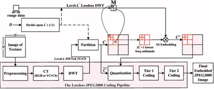
艋L.For embedding, we interrupt the JPEG2000 coding of the texture after the DWT step, as illustrated in Fig.1, and use one of the transformed YCrCb components as a carrier for embedding. The carrier 共C兲 is partitioned into m⫻m equal-sized block, Bi,jwith size dependent on the value of
L
⬘
. If L⬘
= L, then C consists of the whole of the selected component共s兲 and embedding block size remains t⫻t, since no subband is excluded from the possible data inser-tion. Otherwise, for L⬘
⬍L, only a subset of subbands—the lowest 3L⬘
+ 1 of the original 3L + 1 after excluding the re-maining 3共L−L⬘
兲 higher frequency subbands—constituteC, and Bi,j has a reduced size of t/2共L−L⬘兲⫻t/2共L−L⬘兲. Care
must be taken of the fact that block size must be large enough to reliably recover the embedded data after corre-lation. This decision about the choice of L
⬘
is especially important in the case of terrain visualization, where a view-point analysis may be quite useful to ascertain the maxi-mum tolerable error in the DEM that would in turn deter-mine the extent to which the synchronization must be adapted. Hence the important factors in reaching a decision are based on the value of L⬘
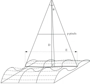
, the block size, and the in-volvement or otherwise more than one YCrCb component in embedding. Our strategy is aimed at the best 3-D visu-alization as a function of the network connection and the computing resources of the client. The proposed adaptive approach to embed the range data in the DWT texture is a function of the distance D between the viewpoint and the depth map. The latter’s quality is evaluated with the root mean square error共RMSE兲 in length units. As pointed out in some recently published works,14even today the acqui-sition of the DEM for 3-D terrain visualization is error prone and it is difficult to get a RMSE less than 1 m. To calculate the maximum acceptable RMSE for an optimal 3-D visualization, we rely on the distance D between the viewpoint and the depth map, as illustrated in Fig. 2, and the visual acuity共VA兲 of the human visual system 共HVS兲.Visual acuity is the spatial resolving capacity of the HVS. It may be thought of as the ability of the eye to see fine details. There are various ways to measure and specify vi-sual acuity, depending on the type of acuity task used. VA is limited by diffraction, aberrations, and photoreceptor den-sity in the eye.15In this work, for the HVS we assume that the VA corresponds to an arc VA of 1 min 共1
⬘
= 1/60 deg兲. Then for a distance D, the level of detail 共LOD兲 is:LOD = 2⫻ D ⫻ tan共VA兲. 共1兲
For example, in the case of terrain visualization, if D = 3 m then LOD= 87⫻10−4 m, and if D = 4 km then LOD = 1.164 m. For our application, illustrated in Fig. 2, if we want to see all the depth map, we have a relation between
D and the size of the range data共width=E m兲:
E = 2⫻ D ⫻ tan共/2兲. 共2兲
Usually the field of view of the HVS is = 60 deg. For example, if E = 3200 m, then D = 2771.28 m.
For 3-D visualization, we should take into account the resolution of the screen in pixels. As illustrated in Fig.2, if we have an image or a screen with p pixels for each row, then the LOD⑀in p is:
⑀= E/2
tan共/2兲⫻ tan共/p兲. 共3兲
With= 60 deg, E = 3200 m, and a resolution of 320 pixels 共for a PDA, for example兲, we have a LOD ⑀= 9.07 m. Then, in this context, for our application we can assume that a RMSE near 9 m is acceptable for the DEM in the case of terrain visualization. Notice that we generate a con-servative bound by placing an error of the maximum size as close to the viewer as possible with an orthogonal projec-tion of the viewpoint on the depth map. We also assume that the range data model is globally flat, and that the ac-curacy between the center and the border of the depth map is the same. In reality, the analysis should be different, and part of the border should be cut as explained by Ref.16in
a particular case of a cylinder. Anyhow, the value of D would help us to reach a decision about the value of L
⬘
.2.2 Embedding Step
The process of embedding is made in a given DWT-domain range data coefficient of the carrier C, which is one or more of the YCrCb components of the transformed texture. The criteria for ascertaining the carrier depends on L
⬘
, t, and, whereis the number of bits assigned to represent a single DWT-domain range data coefficient. If T is the threshold on the number of carrier coefficients needed to embed a single bit, then algorithm 1 proposes a solution to choose only one or three components.Algorithm 1. A subroutine to choose component共s兲 for embedding.
1. If共t2/ 22共L−L⬘兲艌T兲 then
2. select for C one of the three YCrCb components 3. else
4. if共T⬎t2/ 22共L−L⬘兲艌T/ 3兲 then
5. C is constituted by the three YCrCb components
6. else
7. A4S embedding may not be convenient
8. end if 9. end if.
The choice whether to embed in the Y or Cr/Cb plane depends on the fact that Y plane embedding would distort the encoded image, while chrominance plane embedding would escalate the final file size. Neither is the former a serious issue, as embedding is removable, nor is the latter, since it may matter only when L
⬘
= L.The embedding process of a DEM coefficient in a given block 共size=t2/22共L−L⬘兲兲 is elaborated by the flowchart given in Fig. 3. Since one coefficient is embedded per
t/2共L−L⬘兲⫻t/2共L−L⬘兲 block, each Bi,j is repartitioned into as many subblocks 共bk兲 as there are number of bits used to
represent a single transformed coefficient. Each of bkfrom Bi,j would carry the k’th bit k of the transformed range
altitude di,j. Embedding depends on a key generating a
pseudorandom matrix W with entries from the set兵␣, −␣其. The matrix W has the same size as bk, i.e., W =关yuv兴n⫻n,
where yuv苸兵␣, −␣其. The scalar ␣ is referred to as the
strength of embedding. If the bit to embed k is 1, then
matrix W is added to the matrix bk, otherwise W is
sub-tracted from bk. The result is a new matrix bk
⬘
that replaces bkas a subblock in the embedded block Bi,j⬘
of the markedcarrier C
⬘
.Two factors are important here. First is the DWT level 共L
⬘
兲 of transformed range data before embedding, which is a tradeoff between the final texture quality and its range data quality. At the decoding end, the quality of the range data would depend on the difference between L and L⬘
. The larger the difference共L−L⬘
兲, the higher the quality will be θΕ D
ε
p pixels
and vice versa. Second is the value of ␣, since a larger ␣ means high degradation of the watermarked texture. This second factor is, however, of secondary importance since the embedded message共M兲 after recovery will be used to correct any loss in texture quality. So, no matter how much degradation is there, the reconstructed texture should be of the highest possible quality.
2.3 Decoding Step
The prior coded image can be utilized like any other JPEG2000 image and sent across any communication chan-nel. The decoding is more or less converse to the previous process. Just before the inverse DWT stage of the JPEG2000 decoder, the range data can be extracted from
C
⬘
using the previously mentioned partitioning scheme, i.e., Bi,j⬘
blocks and their bk⬘
subblocks. Figure4shows theflowchart for the recovery of a range altitude di,j from
sub-blocks bk
⬘
of Bi,j⬘
and eventual reconstruction of bi,j, andultimately Bi,j. A given k’th subblock bk
⬘
and also the matrixW can be treated as a column/row vector, and the Pearson’s correlation coefficient17can be computed. Ifis closer to −1 than 1, then the embedded bit  was a 0, otherwise it was a 1. Once this is determined, then it is obvious that what were the entries of bk, i.e., ifis 0, then add W to bk
⬘
,otherwise subtract W from bk
⬘
.Algorithm 2. Embedding of the range data coefficient
di,jin the corresponding block Bi,j. 1. Begin
2. get the共i,j兲’th partition Bi,jof the cover and the corresponding
16 bit coefficient di,j
3. partition Bi,jto 16 subblock, b0, b1, . . . b15
4. for k←0 to 15 do
5. read the k’th bitkof the DEM coefficient di,j
6. ifk= 0 then
7. set bk⬘←bk− W/*W is a one-time pseudorandomly
constructed matrix*/
8. else
9. set bkl←b k+ W
10. end if
11. replace bkby bk⬘in the block Bi,j, which will ultimately change
to Bi,j⬘
12. end for
13. replace Bi,jby Bi,j⬘ in the cover 14. end.
2.4 Reconstruction Step
Now comes the reconstruction phase, where by the appli-cation of 0-padding, one can have L + 1 and L
⬘
+ 1 different approximation images of texture and their range data, re-spectively. This is where one achieves the scalability goal.Our method is based on the assumption that it is not nec-essary that all the subbands are available for reconstruction, i.e., only a part of C
⬘
is on hand. This is one of the main advantages of the method, since the range data and the texture can be reconstructed with even a small subset of the coefficients of the carrier. The resolution scalability of wavelets and the synchronized character of our method en-able a 3-D visualization, even with fewer than original res-olution layers as a result of partial or delayed data transfer. The method thus enables us to effect visualization from a fraction of data in the form of the lowest subband of a particular resolution level, since it is always possible to stuff 0s for the higher bands. The idea is to have a 3-D visualization utilizing lower frequency subbands at levelL
⬙
, say, where L⬙
艋L. For the rest of L−L⬙
, part one can always pad a 0 for each of their coefficients. The inverse DWT of the 0-stuffed transform components will yield what is known as an image of approximation of level L⬙
. Before this, as depicted by algorithm 3, data related to the third dimension, i.e., range data, must be extracted whose size depends on both L⬙
and L⬘
. Thus if L⬘
艋L⬙
, one will always have the entire set of the embedded altitude, since all of them will be extractable. We would have a level 0 approximate final range map after inverse DWT of the highest possible quality. On the other hand, if L⬘
⬎L⬙
, one would have to pad 0s for all coefficients of higher L⬘
− L⬙
subbands of a transformed range map before inverse DWT, which would result in a level L⬙
-approximate range data of an inferior quality.Algorithm 3. The reconstruction process via 0-padding.
1. Begin
2. read the coded texture data corresponding to level-L⬙subbands 3. decode to extract the range data that may correspond to L⬙or
a larger level L⬙+⌬, where ⌬艋0 depends on the extent of adaptation
4. for both the texture and extracted range data do
5. initialize clto L⬙if dealing with texture or to L⬙+⌬, otherwise 6. stuff a 0 for every coefficient of the subbands with level⫽cl
7. apply inverse DWT to the result
8. add the result with the共cl− 1兲 approximation to get the 共cl兲
approximation 9. end for 10. end.
3 Experimental Results and Analyses
We have applied our method to examples from two areas, namely terrain and facial visualizations, with the results presented and analyzed in Secs. 3.1 and 3.2, respectively. In Sec. 3.3, we take the allowable limit of adaptation and ap-ply the method to a set of 3-D texture/range data pairs, and analyze the robustness offered by our method.
3.1 Terrain Visualization
We have chosen the example texture/DEM pair given in Fig.5to try various possible adaptations in embedding. We are using a tiling approach: each DEM and texture are de-composed in small parts to facilitate the transfer between the server and clients. The DEM关Fig.5共a兲兴 is shown in the form of a 32⫻32 grayscale image, where the whiteness determines the height of the altitude. The corresponding texture关Fig.5共b兲兴 has a size of 3072⫻3072 pixels, imply-ing one DEM coefficient per 96⫻96 texture block, i.e., t = 96. For the purpose of comparison, a 256⫻256 pixel por-tion, at共1000, 1500兲 coordinates, is magnified as shown in Fig.5共c兲. Figure 5共d兲 illustrates a 3-D view obtained with the help of the texture/DEM pair. We chose to subject the texture to reversible JPEG2000 encoding at L = 4 that would give us five possible resolutions共13 subbands兲 based on 1, 4, 7, and 10 lowest frequency or all of the 13 sub-bands.
For fully synchronous embedding, all 13 subbands of the selected component were utilized in embedding, and thus the DEM was subjected to lossless DWT at level L
⬘
= L = 4 to give 13 subbands. The embedding block Bi,jthen hada size of 96⫻96 for the embedding of one 16-bit trans-formed DEM coefficient, which means a 24⫻24 subblock 共bk兲 per DEM bit. Since bk is large enough, the needed
strength/amplitude 共␣兲 of embedding is smaller and the quality of the luminance/chrominance component will not deteriorate much. For our example, it was observed that 100% successful recovery of the embedded message is re-alized when ␣= 2 for embedding chrominance component 共Cr/Cb兲, as against␣= 8 for embedding luminance compo-nent 共Y兲. The overall quality of the watermarked texture was observed to be better共44.39 dB兲 for Cr/Cb than for Y 共26.53 dB兲. This quality difference is not that important, however, since the original texture is almost fully recover-able from the watermarked texture. On the other hand, there is a risk that embedding in Cr/Cb may eventually inflate the size of the coded image. This risk was, however, not that important for this example, since the observed bi-trate was found to be only marginally escalated in the fully synchronized case—14.81 bpp compared to 14.55 bpp for any adaptation. The texture bitrate is thus independent of the extent of adaptation in partially synchronized cases.
Fig. 3 Flowchart of the DWT domain SS embedding of the depth coefficient di,jin the block Bi,jof the
lowest 3L⬘+ 1 texture subbands.
Fig. 4 Flowchart of the recovery of the depth coefficient di,jand the block Bi,jfrom the SS embedded
This is probably due to the exclusion of the three largest subbands from embedding; these bands, incidentally, have the highest probability of zero coefficients.
On the reintroduction of marked Y or Cr/Cb to the JPEG2000 pipeline, we get our watermarked texture image in JPEG2000 format. From this image one can have five different approximation images for both the DEM and
tex-ture. The level-l共艋L兲 approximate image is the one that is constructed with共1/4l兲⫻100% of the total coefficients that
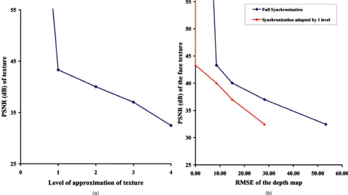
correspond to the available lower 3共L−l兲+1 subbands. For example, a level-0 approximate image is constructed from all the coefficients, and a level-2 approximate image is con-structed from 6.12% of the count of the initial coefficients. Since the embedded data are removable, one gets the high-est possible qualities for all the texture approximations but not for the DEM, as its quality depends on our embedding strategy. Figure6共a兲shows the variations in texture quality as a function of the level of approximation. Since we have been able to extract the texture coefficients with 100% ac-curacy, any quality loss observed after that is not due to the proposed method, but external factors like the nature of texture, or types of wavelet employed by the JPEG2000 codec.
The sensitive nature of DEM compels us to avoid too much loss in its quality. For improved DEM quality, we had to adjust the synchronization, and rather than persisting with L
⬘
= 4, we went for L⬘
⬍4, which meant exclusion of 3共4−L⬘
兲 highest frequency subbands of the carrier from embedding; the synchronization was now maintainable be-tween all the 3L⬘
+ 1 subbands of DEM and the subset 3L⬘
+ 1 lowest subbands of the carrier. Obviously, dimen-sions of Bi,jand bkwere dyadically reduced by a factor of24−L⬘, which led to an increase in the value of ␣ and an eventual degradation in the quality of the coded texture. As described in Sec. 2.3, the most important step of our ap-proach is to adapt the synchronization. In other words, the objective of the step is to find the lower bound for L
⬘
. This bound depends on the texture-to-DEM size ratio and also on how much distortion in the carrier is reversible, i.e., bounds of ␣. For our example, the lowest quality for the coded texture—13.40 dB with ␣= 64 for the Y carrier 关Figs.7共a兲and 7共b兲兴 and 31.47 dB with␣= 16 for the Cr carrier 关Figs.7共c兲and 7共d兲兴—was observed at L⬘
= 1. The reason is that all the information had to be embedded in just(a) (b)
(c) (d)
Fig. 5 Example images:共a兲 32⫻32 DEM, 共b兲 3072⫻3072 pixel tex-ture,共c兲 a 256⫻256 pixel detail of 共b兲, 共d兲 a corresponding 3-D view.
(a) (b)
Fig. 6 Texture quality as a function of:共a兲 level of approximation of texture and 共b兲 RMSE of DEM in meters.
four lowest energy and smallest subbands, implying a size of 3⫻3 for bkwith␣= 64 for the Y carrier and␣= 16 for a
Cr/Cb carrier. Beyond this bound 共L
⬘
= 0, i.e., spatial do-main兲, the block size did not allow for the recovery of the embedded message. Figure6共b兲illustrates the trend in tex-ture quality as a function of the DEM error for various possible values of L⬘
. To judge the DEM quality, root mean square error 共RMSE兲 in meters 共m兲, as explained in Sec. 2.1, was adopted as a measure. It can be observed that for the same texture quality, one can have various DEM quali-ties depending on L⬘
, the level of DEM decomposition be-fore embedding. The smaller the L⬘
, the higher the degree of adaptation in synchronization and hence higher is the resultant DEM quality. With our approach, by using the example given in Fig. 5, the RMSE of the five possible DEM approximations, i.e., levels 0, 1, 2, 3, and 4, were found to be 0, 3.18, 6.39, 11.5, and 22.88 m, respectively. For full synchronization, as presented in Ref.9, the worst DEM quality, 22.88 m, results when one goes for a 3-D visualization from level-four approximate texture, as the corresponding DEM will also be four-approximate. But even with one step adjustment, this quality is twice im-proved, and for L⬘
= 3, both the three and four approximate texture images have three approximate DEM with RMSE = 11.5 m. Go a step further, and the maximum DEM error will be reduced to 6.39 m. Hence with adaptive synchroni-zation, one can have a high quality DEM even for very low quality texture or, more precisely, the same quality DEMfor all the approximation images at levels 艌L
⬘
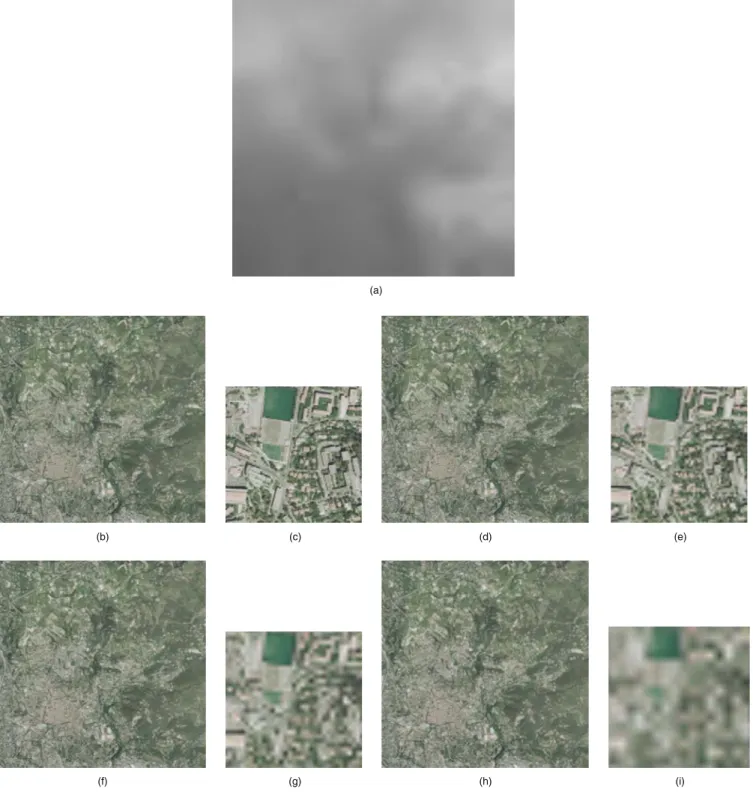
. Figure 8 shows the trend in texture quality for a given DEM error 共3.18 m兲 as a function of bitrate. For the sake of compari-son, we also show the graph when the texture and its DEM are coded separately. A level-one approximate separately encoded DEM corresponds to 0.36 bpp, and this is exactly the escalation for each point on the graph. In other words, for the example in hand, our method can give an advantage of 0.36 bpp in bitrate for a given PSNR. Note that we can have a texture/DEM pair with even a bitrate as low as 0.06 bpp and even 0.27 bpp with our method. Images cor-responding to a DEM error of 3.18 m are shown in Fig.9 and the resultant 3-D visualizations are illustrated in Fig. 10. It can be seen that with even a tiny fraction of the total coefficients关as low as 0.40%, i.e., Figs.9共h兲and9共i兲, and Fig.10共e兲兴, a fairly commendable visualization can be re-alized.The maximum error in RMSE of the DEM tolerable by an observer is a function of the distance of the observer, i.e., the viewpoint D. This threshold is mainly dependent on the human visual system 共HVS兲 and for this reason, the analysis given in Sec. 2.1 is extremely useful to adapt the synchronization.
3.2 Application to Three-Dimensional Face
Visualization
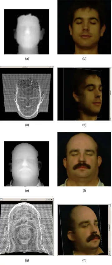
For comparable dimensions of the texture and depth map, we opt for a face visualization example. In this context, we applied our method to a set of examples of more 100 mod-els from the FRAV3D18 database, each consisting of a 512⫻512 face texture and a corresponding 64⫻64 depth map of 8-bit coefficients. Two examples are given in Fig. 11. Thus one depth map coefficient corresponds to an 8 ⫻8 texture block, which means that the margin for adapta-tion is narrow. Hence, even if we involve all the three planes共i.e., YCrCb兲 in embedding, we can adapt, at most, by one level with a SS embedding. The 8-bit depth map
(a) (b)
(c) (d)
Fig. 7 Texture after embedding in:共a兲 Y plane 共␣= 64兲 with PSNR = 13.40 dB, 共b兲 its 256⫻256 detail, 共c兲 Cr plane 共␣= 16兲 with PSNR= 31.47 dB, and共d兲 its 256⫻256 detail.
Fig. 8 Comparison between the proposed method and separate coding for the variation in texture quality as a function of its bitrate for a DEM error of 3.18 m.
was subjected to level-L
⬘
lossless DWT before embedding in the three DWT-domain components from the JPEG2000 coder. To ensure accuracy, we expand the word size for each of the transformed depth map coefficients by one ad-ditional bit, and represent it in 9 bits that are then equally distributed among the three planes for embedding. TakingL = 4 would imply L
⬘
= 4 for synchronous embedding, andL
⬘
= 3 for a one-level adaptation in synchronous embed-ding. To embed one bit, the former would manipulate about 21 while the latter about five coefficients of Y, Cr, or Cb plane in the DWT domain.For the set of face examples, the maximum of the lowest value of␣needed for the 100% recovery of the embedded data was found to be 26 for the synchronous case and 45
(a)
(b) (c) (d) (e)
(f) (g) (h) (i)
Fig. 9 Approximations corresponding to the 3.18-m error DEM共L−1 approximate兲: level-L⬘DEM is embedded in the lowest 3L⬘+ 1 DWT domain subbands of level-four Cr-texture.共a兲 L−1 DEM, 共b, c兲 L − 1 approximate texture共4.29 bpp兲 with L⬘= 4,共d, e兲 L−2 approximate texture 共1.1 bpp兲 with L⬘= 3,共f, g兲 L−3 approximate texture 共0.27 bpp兲 with L⬘= 2,共h, i兲 L−4 approximate texture 共0.066 bpp兲 with L⬘= 1.
for the adaptive synchronous case. The resultant water-marked JPEG2000 format image was degraded to a mean PSNR of 17.15 dB for the former and a mean PSNR of 15.16 dB for the latter. Even with that much distortion, the reversible nature of the method enabled us to fully recover the embedded data on one hand and achieve the maximum possible quality in case of the texture, i.e., with a PSNR of infinity, on the other. Figure12共a兲plots the PSNR against the level of approximation for the reconstruction of texture. It can be seen that even a texture reconstructed with as low as 0.39% of the transmitted coefficients has a PSNR of around 30 dB. The advantage of adaptation is evident from the fact that, as shown in Fig. 12共b兲 for the same texture quality, even one-level adaptation offers far better depth map quality compared to full synchronization.
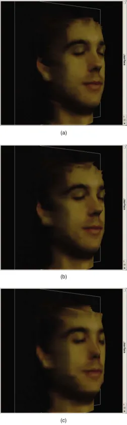
The evident edge of the adaptive strategy in depth map quality is conspicuous by the comparison of 3-D visualiza-tions illustrated in Figs. 13 and 14. The latter is always better by one level共four times, roughly兲 as far as depth map quality is concerned. Hence with the same number of trans-mitted coefficients, one gets the same level-l approximate texture for the two cases, but the one-level adaptive case would have a level-l − 1 approximate depth map compared to the relatively inferior level-l approximate depth map for the fully synchronized case.
3.3 Robustness Analysis
The main purpose of employing an SS strategy was to im-prove the robustness of the embedded texture against noisy transmission and image manipulation. In the latter case, attacks are typically aimed at the change of image format, e.g., to JPEG, and cropping. We believe that our method
(a)
(b) (c)
(d) (e)
Fig. 10 3-D visualization corresponding to Fig.9.共a兲 L−1
approxi-mate DEM-3.18-m error, 共b兲 L − 1 approximate texture
共L⬘= 4兲—4.29 bpp, 共c兲 L−2 approximate texture 共L⬘= 3兲—1.1 bpp, 共d兲 L−3 approximate texture 共L⬘= 2兲—0.27 bpp, and 共e兲 L−4 ap-proximate texture共L⬘= 1兲—0.066 bpp.
(a) (b)
(c) (d)
(e) (f)
(g) (h)
Fig. 11 Two examples of face visualization: 共a兲 and 共e兲 64⫻64 depth maps,共b兲 and 共f兲 512⫻512 pixel face textures, 共c兲 and 共g兲 the corresponding 3-D meshes, and共d兲 and 共h兲 3-D views.
gives us the sought-after robustness. In this section we are subjecting the marked texture to various manipulations to ascertain the claimed robustness. For the sake of brevity, we use the nomenclature described in Table1to represent various manners of the DWT domain embedding of the range data in the texture, e.g., desynY implies DWT do-main embedding of range data coefficients in the Y plane of texture, excluding the three highest frequency subband co-efficients共75% of the total兲.
Our method was applied to a set of 300 tiles correspond-ing to the region of Bouches du Rhône in France provided by IGN,19 Paris, France. All the tiles were composed of a 1024⫻1024 pixel texture and a corresponding DEM of 32⫻32 16-bit altitudes. All the textures were subjected to level-four 共L=4兲 decomposition in the JPEG2000 codec. The DEM were DWTed at level L
⬘
= 4 for synY and synCr, and L⬘
= 3 for desynY and desynCr. For each pair we deter-mined the minimum of␣needed for 100% recovery of the embedded coefficients. For all such␣’s, we determined the minimum共␣min兲 and maximum 共␣max兲 in the set images for each case, as given in Table2. It can be observed from the PSNR values given in the table that the Y-plane embedding and larger␣distort the texture more. Although the embed-ded message is fully removable, we still need to maintain the quality of the encoded texture, and that is why we settled for different␣maxfor each case. Otherwise, the glo-bal maximum ␣max= 49 would have been a better choice. Hence, for the sake of comparison, we then carried out embedding in the example set of textures at␣max conform-ing to Table2 for each of the four embedding cases. The watermarked JPEG2000 coded textures were then subjected to robustness attacks.3.3.1 Resistance to JPEG compression
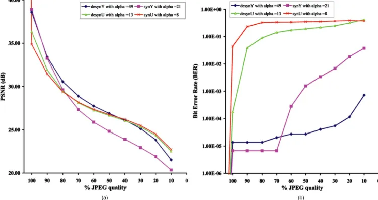
To show the intensity of the JPEG compression, we have plotted the average PSNR of the distorted texture against the quality factor of compression, as shown in Fig.15共a兲. It can be observed that for all four cases, the trend is identi-cal, although the desynY case performs comparatively bet-ter at higher qualities. But since the embedding is remov-able, it is the integrity of the embedded data, i.e., DEM, which is important and that is why we have plotted the average bit error rate 共BER兲 of the recovered DEM as a function of the JPEG quality factor in Fig.15共b兲. The rea-son is that the abscissa going beyond 100% is for the pur-pose of representing the no-attack case, which must have a BER of zero. It can be observed that cases most sensitive to JPEG compression are the cases where embedding was car-ried out in the chrominance plane 共desynCr, synCr兲, and even 100% quality factor of compression can result in sig-nificant errors. In contrast, Y-plane embedding offers high robustness, with desynY being the most robust.
3.3.2 Robustness against Gaussian noise addition
The amount of distortion as a result of the Gaussian noise can be judged from Fig. 16共a兲, where the embedding in-volving the U/V plane is least distorted, but again it is the quality of the retrieved DEM that matters. We have sub-jected the watermarked textures to a zero-mean Gaussian noise at standard deviations 共s兲 in the range 0.1 to 50. Figure 16共b兲 shows the graph where the mean BER is plotted as a function of , with both axes drawn on a
(a) (b)
Fig. 12 Variation in the texture quality as a function of:共a兲 its approximation level and 共b兲 RMSE of the extracted depth map.
logarithmic scale. In general all the cases are robust until about = 0.8, which is quite a large value. Beyond this value, robustness varies from case to case, with the fully synchronous cases being the most robust.
3.3.3 Prospects of cropping
The robustness demonstrated is equally valid for cropping, and we have been able to recover all the coefficients em-bedded in a cropped patch, provided that the following con-straints were met:
(a)
(b)
(c)
Fig. 13 Overlaying level-l approximate texture on the extracted level-l approximate depth map:共a兲 level 1, 共b兲 level 2, and 共c兲 level 3.
(a)
(b)
(c)
Fig. 14 Overlaying level-l approximate texture on the extracted level共l−1兲 approximate depth map: 共a兲 level 1, 共b兲 level 2, and 共c兲 level 3.
1. The cropped patch has dimensions that are multiples of PD, where: PD =
冉
1 + 3兺
i=0 L−1 4i冊
1/2 ⫻ t/2共L−L⬘兲. 共4兲 2. Each patch coordinate during the cropping must be amultiple of PD.
Calculating PD is necessary, since the embedding is done in the level-L DWT domain, and one would need the whole tree corresponding to a given coefficient. We know that each tree has as its root a coefficient from the lowest frequency subband and a set of sibling nodes. The root has three child nodes and each child, with the exception of leaves, has four child nodes. On part of the watermarked texture, all this amounts to an area of 1 + 3兺i=0L−14
i
times the texture block size used for embedding each coefficient, which is equal to t/2共L−L⬘兲⫻t/2共L−L⬘兲.
The recovery of the DWT-domain DEM has always been in its entirety, but here comes another hurdle—the
classical image boundary problem—which prevents us from getting the exact inverse DWT. JPEG2000 has been supporting two kinds of transforms:20,21 the reversible integer-to-integer Daubechies 共5/3兲 and the irreversible real-to-real Daubechies共9/7兲, with the former being loss-less and the latter being lossy. The standard follows a lifting approach,21,22for DWT in a separable rather than nonsepa-rable manner, and approximations are inevitable at bound-aries. In 2-D, the upper and lower boundaries of a given subband have to be approximated both horizontally and vertically. The module for inverse DWT usually takes into account these approximations, and the inverse must be ex-actly the same as the initial if the transform is supposed to be reversible. It is here that our problem starts, because even though we have recovered all the coefficients without any error, the inverse transform will still yield false coeffi-cients at subband interfaces and borders. These errors are not affordable, as DEM is critical data. To elaborate further, let us take a visualization scenario where a number of tex-ture images are to be tiled together for the visualization of
Table 1 Nomenclature.
Name synY synCr desynY desynCr
Embedding plane Y CrCb Y CrCb
L − L⬘ 0 0 1 1
Excluded subbands Nil Nil LH1, HL1, HH1 LH1, HL1, HH1
Table 2 Extreme values of␣for various embedding scenarios.
Case synY synCr desynY desynCr
␣min 12 32 4 10 ␣max 21 49 8 13 Mean PSNR 共coded texture兲 18.25dB 12.90 dB 32.94 dB 30.23 dB (a) (b)
Fig. 15 Robustness of the embedded texture to JPEG compression:共a兲 texture quality and 共b兲 range data quality.
a very large area. If we are focused at a single tile, its visualization may be rendered at full resolution but its eight neighboring tiles need not be visualized at full resolution if resources are limited. Now if suddenly the focus is changed or expanded共the observer recedes back兲, parts of the neigh-boring tiles have to be visualized. These parts will always correspond to corners of one or more neighboring tiles, and it is here our method can be helpful, since with our ap-proach corners can more reliably be visualized via crop-ping. Figure17graphically illustrates different focus situa-tions, with the circle representing the focus and the rectangle with broken borders representing the minimum area that must be rendered for visualization.
Let us suppose the Grand Canyon example is to be ren-dered at the bottom-right tile in the situation given in Fig. 17共a兲. Let the needed upper left corner corresponds to an area less than 256⫻256 pixels. Let the texture embedded synchronously at L = 2, which would mean in light of the discussion in the beginning of this section, that after
extrac-tion from a 256⫻256 pixel texture patch and then inverse DWT, the DEM patch would be accurate but for the last three rows and columns of the coefficients. Figure18 com-pares the 3-D visualization obtained by decoding and ex-tracting the cropped patch by our method with that obtained from the original DEM corresponding to the patch. 4 Conclusion
In this work we present an efficient adaptive method to hide 3-D data in a texture file to have a 3-D visualization and to transmit data in a standardized way, defined by the open Geospatial Consortium.23The proposed method has the pe-culiarity of being robust and imperceptible, simultaneously. The high strength of embedding goes somewhat against security, but that has never been the goal. With adaptation in synchronization, higher quality of the depth map is en-sured, but the extent of adaptation is strictly dependent on the embedding factor. The more the range data size
ap-(a) (b)
Fig. 16 Robustness to a zero-mean Gaussian noise at various standard deviations共兲: 共a兲 texture quality and共b兲 range data quality.
Original viewpoint Original viewpoint New viewpoint Shift New viewpoint Original viewpoint Receding (a) (b) (c)
proaches that of the texture, one is compelled to elevate the strength of embedding, and if the trend goes, the prospect of using SS embedding may gradually diminish before in-volving more than one YCrCb planes in embedding.
The quality offered by the method for various approxi-mations is the ultimate, as 100% of the texture and depth map coefficients are recoverable. Beyond that, one would have to look forward to the use of some other, more effi-cient special wavelet transforms in the JPEG2000 codec by engineering some plug-in. Ideally, these wavelets must of-fer the lowest quality gap between the various resolution levels. The robustness studies seem to be really interesting, especially in the case of cropping, where an effort is made to realize a 3-D visualization with a small patch cropped from the encoded image. One of our future undertakings should underline the need to further investigate the robust-ness, with special reference to the cropping scenario dis-cussed. In addition, our perspective must include the study of the focus of the viewpoint.
Acknowledgments
This work is in part supported by the Higher Education Commission共HEC兲, Pakistan.
References
1. K. W. Bowyer, K. Chang, and P. Flynn, “A survey of approaches and challenges in 3D and multi-modal 3D + 2D face recognition,” Com-put. Vis. Image Underst.101共1兲, 1–15 共2006兲.
2. C. Conde and A. Serrano, “3D facial normalization with spin images and influence of range data calculation over face verification,” Proc. Conf. on Computer Vision and Pattern Recognition, vol. 16, pp. 115– 120, IEEE Computer Soc., Washington, DC共2005兲.
3. M. P. Gerlek, The “GeoTIFF Box” Specification for JPEG 2000 Metadata–DRAFT version 0.0, LizardTech, Inc., Seattle共April 2004兲. 4. R. Lake, D. Burggraf, M. Kyle, and S. Forde, GML in JPEG 2000 for Geographic Imagery (GMLJP2) Implementation Specification, Num-ber OGC 05-047r2, Open Geospatial Consortium共OGC兲 共2005兲. 5. See http://www.remotesensing.org/geotiff/spec/contents.html. 6. S. Weik, J. Wingbermuhle, and W. Niem, “Automatic creation of
flexible antropomorphic models for 3D videoconferencing,” in Proc. Computer Graphics Intl. (CGI’98), pp. 520–527, IEEE Computer Soc., Washington, DC共1998兲.
7. See http://www.tixeo.com.
8. D. Q. Dai and H. Yan, “Wavelets and face recognition,” in Face
Recognition, I-Tech Education Publishing, Vienna, Austria共2007兲. 9. K. Hayat, W. Puech, and G. Gesquière, “Scalable 3D visualization
through reversible JPEG2000-based blind data hiding,”IEEE Trans. Multimedia10共7兲, 1261–1276 共2008兲.
10. J. Royan, P. Gioia, R. Cavagna, and C. Bouville, “Network-based visualization of 3D landscapes and city models,” IEEE Comput. Graphics Appl.27共6兲, 70–79 共2007兲.
11. P. Gioia, O. Aubaut, and C. Bouville, “Real-time reconstruction of wavelet encoded meshes for view-dependent transmission and visu-alization,”IEEE Trans. Circuits Syst. Video Technol. 14共7兲, 1009– 1020共2004兲.
12. J. K. Kim and J. B. Ra, “A real-time terrain visualization algorithm using wavelet-based compression,”Visual Comput.20共2–3兲, 67–85 共2004兲.
13. I. J. Cox, M. L. Miller, and J. A. Bloom, Digital Watermarking, Morgan Kaufmann Publishers, New York共2002兲.
14. U. Vepakomma, B. St. Onge, and D. Kneeshaw, “Spatially explicit characterization of boreal forest gap dynamics using multi-temporal lidar data,”Remote Sens. Environ.112共5兲, 2326–2340 共2008兲. 15. G. Smith and D. A. Atchison, The Eye and Visual Optical
Instru-ments, Cambridge University Press, New York, USA, 1997. 16. W. Puech, A. G. Bors, I. Pitas, and J. M. Chassery, “Projection
dis-tortion analysis for flattened image mosaicing from straight uniform generalized cylinders,”Pattern Recogn.34共8兲, 1657–1670 共2001兲. 17. W. S. Moore, The Basic Practice of Statistics, W. H. Freeman Co.,
New York共2006兲.
18. See http://www.frav.es/databases/FRAV3d/. 19. See http://www.ign.fr.
20. I. Daubechies and W. Sweldens, “Factoring wavelet transforms into lifting steps,”Fourier Anal. Appl.4共3兲, 247–269 共1998兲.
21. W. Sweldens, “The lifting scheme: a new philosophy in biorthogonal wavelet constructions,”Proc. SPIE2569, 68–79共1995兲.
22. S. Mallat, A Wavelet Tour of Signal Processing, Academic Press, San Diego, CA共1998兲.
23. See http://www.opengeospatial.org 共special care must be taken on standards W3D and WVS兲.
Khizar Hayat received the MSc共chemistry兲 degree from the Univer-sity of Peshawar, Pakistan, in 1993. He worked as a lecturer in the Higher Education Department, Khyber Pakhtunkhwa, Pakistan, from 1995 to 2009. During this period, he was awarded a scholarship in 2001 by the Government of Pakistan to persue an MS degree in computer science from Muhammad Ali Jinnah University, Karachi, Pakistan. He also received the Master 2 by Research共M2R兲 degree in computer science from the University of Montpellier II 共UM2兲, France. In June 2009, he did his PhD while working at LIRMM 共UM2兲 under the supervision of William Puech 共LIRMM兲 and Gilles Gesquière共LSIS, University of Aix-Marseille兲 with a scholarship from The Higher Education Commission of Pakistan. He has recently joined COMSATS Institute of Information Technology共CIIT兲 Abbot-Fig. 18 3-D visualization from a patch cropped from a Y-embedded texture.
tabad, Pakistan, as an assistant professor. His areas of interest are image processing and information hiding.
William Puech received the diploma of electrical engineering from the University of Montpellier, France, in 1991, and the PhD degree in signal image speech from the Polytechnic National Institute of Grenoble, France, in 1997. He started his research activities in im-age processing and computer vision. He served as a visiting re-search associate to the University of Thessaloniki, Greece. From 1997 to 2000, he was an assistant professor in the University of Toulon, France, with research interests including methods of active contours applied to medical image sequences. Between 2000 and 2008, he was an associate professor, and since 2009, he has been a full professor in image processing at the University of Montpellier, France. He works in the Laboratory of Computer Science, Robotics, and Microelectronics of Montpellier共LIRMM兲. His current interests
are in the areas of protection of visual data共image, video, and 3-D objects兲 for safe transfer by combining watermarking, data hiding, compression, and cryptography. He has applications for medical im-ages, cultural heritage, and video surveillance. He is the head of the Image and Interaction team and he has published more than ten journal papers, four book chapters, and more than 60 conference papers. He is a reviewer for more than 15 journals and for more than ten conferences. He is an IEEE and SPIE member.
Gilles Gesquière is currently an assistant professor at the LSIS Laboratory, Aix-Marseille University, France. He obtained his PhD in computer science at the University of Burgundy in 2000. His re-search interests include geometric modeling, 3-D visualization, and deformation. He is currently working on projects focused on 3-D geographical information systems.