Comparative Analysis of Two Online Identification Algorithms in
a Fuel Cell System
M. Kandidayeni1*,A. Macias1,A. A. Amamou1, L. Boulon1,2, S. Kelouwani1
1Université du Québec à Trois-Rivières, Hydrogen Research Institute, Trois-Rivières, QC,
Canada
2Canada Research Chair in Energy Sources for the Vehicles of the Future
present address:3351 Boulevard des Forges, Trois-Rivières, QC G9A 5H7, Canada
Abstract
Output power of a fuel cell (FC) stack can be controlled through operating parameters
(current, temperature, etc.) and is impacted by ageing and degradation. However, designing a complete FC model which includes the whole physical phenomena is very difficult owing to its multivariate nature. Hence, online identification of a FC model, which serves as a basis for global energy management of a fuel cell vehicle (FCV), is considerably important. In this paper, two well-known recursive algorithms are compared for online estimation of a multi-input semi-empirical FC model parameters. In this respect, firstly, a semi-empirical FC model is selected to reach a satisfactory compromise between computational time and physical meaning. Subsequently, the algorithms are explained and implemented to identify the parameters of the model. Finally, experimental results achieved by the algorithms are
discussed and their robustness is investigated. The ultimate results of this experimental study indicate that the employed algorithms are highly applicable in coping with the problem of FC output power alteration, due to the uncertainties caused by degradation and operation
condition variations, and these results can be utilized for designing a global energy management strategy in a FCV.
Keywords: Fuel cells, Global energy management, Online identification, Recursive algorithms, Semi-empirical calculations
1 Introduction
Proton exchange membrane fuel cell (PEMFC) is a promising alternative energy conversion device in automotive applications, due to high efficiency and low adverse environmental impacts [1]. Fuel cell vehicles (FCVs) have shown a steady increase in the automotive
market. However, their successful market penetration requires more improvement in terms of performance, reliability, and cost [2]. Hybridization of PEMFC with other sources, such as batteries, and supercapacitors (SCs), has been suggested as an effective measure to improve the mentioned factors in a FCV. Common structures for hybridization of FCVs are FC-battery, FC-SC, and FC-battery-SC. All of these structures have their own advantages and disadvantages [3]. With all the favorable aspects of hybridization, the overall performance of FCVs, regarding fuel and energy consumption, still relies on the powertrain components efficiency and accurate coordination of sources. In this regard, several energy management strategies (EMSs), namely rule-based, optimization-based, and intelligent-based, have been proposed for the mentioned hybrid structures in the literature [4-6]. Some examples of very recent proposed online EMSs can be found in [7-11]. In [7], an online EMS based on data fusion approach is suggested. Three FLCs are then optimized and adapted, by Dempster-Shafer evidence theory, to three driving conditions predicted by support vector machine. However, the design constraints of the controllers come from a static efficiency-power map of a PEMFC. In [8], an adaptive control method, based on tuning the FLC parameters for
different conditions, is proposed. This work remarks on the decline of PEMFC output voltage due to degradation and suggests the rule base values modification under this condition. In [9], an online EMS based on extremum seeking method is suggested to maintain the PEMFC operating points in high efficiency region by means of a band-pass filter. A two-layer EMS composed of rule-based approach and particle swarm optimization has been proposed for real-time control of FCVs in [10]. The rule-based of this work is based on a static PEMFC map. In [11], an EMS based on short-term energy estimation is developed to maintain the SC state of
energy within a defined limit. The PEMFC limits are based on a quasistatic model, and determining the power rate limits to avoid premature ageing is pointed out as a remaining issue.
Literature consideration shows that many of the existent EMSs in the literature are based on parametric PEMFC models, especially static models [12-14]. However, the performance of PEMFCs is influenced by the operating conditions variation (temperature, pressure, current, etc.), degradation, and ageing phenomena. Such performance drifts have made the design of a complete PEMFC model immensely complicated. There exists various PEMFC models capable of dealing with the variations of the operating conditions [15-19]. These models are by some means convincing, though not perfect, with regard to coping with the operating conditions variations. However, ageing phenomena modelling, which is a very complicated process, has not been resolved yet. In this respect, some researches have been conducted to track the real performance of a fuel cell system online. These works can be divided into two categories. The first category is based on extremum seeking strategies, such as maximum power point tracking [20-23]. The second category is based on a parametric identification coupled with an optimization algorithm. This approach is based on models and offers two solutions: 1) a straight solution is to use a model which considers the multi-physics behavior of the PEMFC. As previously mentioned, such a model is itself a study limitation; 2) the second solution is to utilize an online parameter estimation for a grey-box or black box model. Several studies have made a contribution concerning the online identification coupled with an optimization of PEMFC to obtain the best performance. Ettihir et al. have proposed the utilization of a semi-empirical model, which is only a function of current, with a recursive least square method to get the characteristics of the PEMFC online [24]. They have integrated their work into the EMS design of a FCV as well, and achieved interesting results [25-27]. Kelouwani et al. have suggested an experimental study based on tracing the maximum efficiency of the PEMFC. In this study, a polynomial model of the PEMFC efficiency is
introduced and the best efficiency is looked after by adjusting the control variables [28]. Methekar et al. have introduced an adaptive control of a fuel cell system with a Wiener model [29]. Dazi et al. have developed a predictive control to ascertain the maximum power
operation of a fuel cell system [30]. In [31], an adaptive supervisory control strategy for a FC-battery bus based on equivalent consumption minimization is proposed. In this paper, an algorithm has been used for charge-sustaining and a recursive least square has been employed for performance identification of the PEMFC. The utilized PEMFC model of this work is a single input semi-empirical model, which is only a function of current. The studied papers indicate that many online and real-time EMSs have been proposed for FCVs. However, only a few of them, like [24-27, 31], have tried to take into account the real characteristics of the PEMFCs.
This paper aims at providing a basis for easy integration of a PEMFC real behavior into the design of real-time EMSs. In this regard, two recursive algorithms are introduced, and tested to identify the parameters of a semi-empirical model online. This integration provides one with online characteristics of a PEMFC, such as polarization curve, maximum power, and efficiency, which can be used in an EMS loop to update the constraints and related control laws. Compared to other works, the main contribution of this work is online parameters estimation of a multi-input (current, temperature, and pressure) semi-empirical model, which has eight parameters, simultaneously, as opposed to a single-input (current) model with four parameters used in [24-27, 31]. Since the intrinsic dynamic of current, temperature, and pressure are completely different, a multi-input model identification is more challenging than a single-input one. Moreover, a careful experimental study for comparing the effectiveness of the utilized identification methods is given along with a step-by-step explanation for adapting the algorithms to this particular problem. It should be noted that the employed PEMFC model in this work is a combination of the models introduced in [32-34]. The parameters of such model have been only estimated offline with various optimization algorithms in previous
studies [35-39]. However, in this work, parameter identification is performed online to counteract uncertainties that occur slowly over time, such as ageing, and quickly due to change of the operating conditions which are not considered in the model. The remainder of this paper is organized as follows. The explanation on how the proposed method of this work can be integrated into EMS design is given in section 2. The PEMFC model is presented in section 3. Section 4 deals with the explanation of identification algorithms. The obtained results of the work are discussed in section 5. Finally, the conclusion is given in section 6.
2 Integration into energy management design
The EMS of a multi-source system, like a FCV, can be designed in a way to increase system efficiency, lifetime, and autonomy by defining the operating points of the components. However, defining the operating points in a PEMFC is challenging since they steadily move across the operating space. With regard to FCVs, it is interesting to run the PEMFC at its efficient power range. As discussed earlier, many of the designed EMSs in the literature have used some constraints such as the maximum and minimum power range of the PEMFC. However, the power-current profile of a PEMFC changes due to the effect of operating conditions, such as temperature, and other disturbances like ageing phenomena. The variation of PEMFC characteristics acts like uncertainties in EMSs. When these variations are not tracked, they cause mismanagement in the EMS since they change the assumed limits in the controller. In this regard, this section describes how the results of this work can be included in the design of a global energy management in a FCV. The whole process is conducted online while the PEMFC is under operation. The global EMS comprises three stages, namely parameter identification, information extraction, and power split strategy. The objective is to do an online parameter identification to adapt the model to the performance drifts of the
PEMFC, and then define the best operating points in the information extraction stage. Afterwards, the obtained data can be used in the power split strategy stage to control the power flow between the sources. This three-stage process is called global EMS, and is shown in Figure 1. It should be noted that this paper mainly deals with the design of the first two stages, which are the core of the explained global EMS. In fact, this paper focuses on the implementation of the recursive algorithms for estimating the parameters of a semi-empirical PEMFC model online, which is the first stage. Subsequently, the output of the identification process is employed for finding the maximum power of the PEMFC at each moment, which is the second stage. Finding the maximum power in the information extraction step is one given
example out of several possibilities, such as maximum efficiency point (ηmax), minimum
voltage (Vmin), maximum current (Imax), and so forth. The future works can use the provided
basis in this article to design an online power split strategy.
Figure 1: Global Energy Management (I, T, and P refer to operating current, temperature, and pressure respectively).
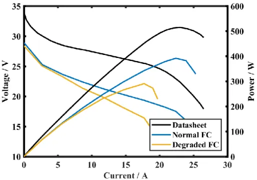
In order to show the importance of taking the real behavior of the PEMFC into consideration, two PEMFCs with different levels of degradation are used in this paper. The exact age of each
PEMFC has not been properly tracked. However, the polarization curves and the maximum deliverable powers of each PEMFC are shown in Figure 2, as a method of distinguishing the current state of each one. As it is observed, the rated power of one of the PEMFCs is almost 400 W while the other one is 300 W. Throughout this manuscript, the less aged PEMFC, which has a higher rated power, is called Normal PEMFC, and the more aged one with less rated power is called Degraded PEMFC. The characteristics of a brand-new PEMFC, which has been obtained from the data sheet, are represented in Figure 2 as well to clarify the difference between the employed PEMFCs in this work and a new one.
Figure 2: Polarization and power curves of new (from data sheet), Normal, and Degraded PEMFCs.
It should be noted that the experimental polarization curves have been obtained by drawing a fixed current from the fuel cells and measuring their output voltage. By slowly stepping up the load, the fuel cell voltage response can be seen and recorded. After each increase in the level of current, 15 to 25 minutes have been allowed to the fuel cells to reach equilibrium. All the tests have been conducted in a stable environment in the test center of Hydrogen Research Institute (IRH) of Université du Québec à Trois-Rivières to maintain the conditions. Another
point which needs to be mentioned is that the employed PEMFCs in this work are Horizon H-500 PEMFCs. The characteristics of a Horizon H-H-500 PEMFC is listed in Table 1. The difference between the rated power, shown in Table 1, and the utilized PEMFCs is due to the degradation. According to manufacturer, the H2 pressure should be regulated between 0.5 to 0.6 Bar. Hence it can be stated that in the utilized air-breathing PEMFCs, the pressure is constant.
Table 1: Horizon H-500PEMFC characteristics
PEMFC Technical specification
Type of FC PEM
Number of cells 36
Active area 52 cm2
Rated Power 500 W
Rated performance 22 V @ 23.5 A
Max Current (shutdown) 42 A
Hydrogen pressure 50-60 kPa (0.5-0.6 Bar)
Rated H2 consumption 7 l min
Ambient temperature 5 to 30 °C
Max stack temperature 65 °C
Cooling Air (integrated cooling fan)
3 Fuel cell modelling
An electrochemical based PEMFC model has been utilized in this paper. In this type of
model, the output voltage of FC (VFC) is considered as the sum of cell reversible voltage
(ENernst) and voltage drops, namely activation (Vact), ohmic (Vohmic), and concentration or mass
transport (Vcon). This type of model considers the same behavior for all the cells. The general
formulation of an electrochemical FC model is as follows:
Where the unit of VFC and the voltage drops is volt and n is the number of cells. In this work, ENernst, which is the potential of FC without load in an open circuit, is calculated based on the following theoretical formula, proposed in [33].
ENernst = 1.229 – 0.85×10⁻³ (T – 298.15) + 4.3085 × 10⁻⁵ T[ln(PH2) + 0.5ln(PO2)] (2)
Where T is the stack temperature / K, PH2, and PO2 are the partial pressure / Pa of hydrogen in
anode side and oxygen in cathode side. Vact is obtained by means of Eq. (3), introduced in
[33].
Vact = ϒ1 + ϒ2T + ϒ3Tln(CO2) + ϒ4Tln(i) (3)
CO2 = PO2/5.08×106 e-(498/T) (4)
Where i is the FC operating current / A, CO2 is the oxygen concentration / mol cm-3, and the
ϒn (n = 1 … 4) is the empirical coefficients, based on fluid mechanics, thermodynamics, and
electrochemistry and may differ depending on the cell material and manufacture.
The formulation of Vohmic, shown in Eq. (5), is based on the proposed structure in [34]. This
structure introduces an appreciable method to avoid struggling with the computation of water content and distribution. Eq. (5) is a function of temperature, due to the fact that diffusivities and water partial pressures change with temperature, and current, since proton and water fluxes alter with the current.
Vohmic = -iRinternal = -i(ξ1 + ξ2T + ξ3i) (5)
Where ξn (n = 1 … 3) are the parametric coefficients. The range of the parameters of ohmic
internal resistor has been obtained by current interrupt test, which is explained later in this
section. Vcon is computed with the help of Eq. (6), proposed in [32, 40].
Vcon = αIGln(1 – βId) (6)
Where α is a semi-empirical parameter related to the diffusion mechanism and it is between
0.3 to 1.8 [23], Id is the current density / Acm-2, G (between 1 and 4) is a dimensionless
number which is related to the water flooding phenomena, and β is the inverse of the limiting
current density / A-1cm2. The value of β is 1.2381.
The introduced PEMFC model comprises 8 time-varying parameters, which need to be identified. In order to embrace the influence of degradation phenomenon, which happens slowly over time, and the operating conditions, which are not included in the model like humidity, the parameters should be identified online to adapt the model to real state of the PEMFC. Table 2 shows the targeted parameters for identification and their expected range of variation. The reported ranges have been adopted from previous studies [35-39], and the obtained values for the parameters of the employed PEMFC in this work may be slightly different. This deviation in the range is mainly due to the various used material in the fuel cells, fabrication methods, state of health of the reported fuel cells, and so forth.
Table 2: Targeted Parameters for estimation
Parameters Range Minimum Maximum ϒ1 -1.997 -0.8532 ϒ2 0.001 0.005 ϒ3 3.6×10⁻⁵ 9.8×10⁻⁵ ϒ4 -2.6×10⁻⁴ -0.954×10⁻⁴ α 0.0135 0.5 ξ1
Current interrupt test ξ2
3.1 Resistor measurement
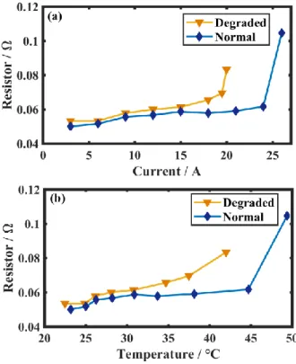
In order to relate the targeted parameters for estimating the internal resistor of the PEMFC to the realistic physical meaning, some measurements from the real value of resistor are needed. Therefore, in this paper, the current interrupt method is used as an electrochemical technique to obtain a range for the resistor variation with regard to current and temperature [41-44]. The efficacy of this method for measuring the ohmic resistance has been already investigated in [44]. Current interrupt test revolves around the idea of rapid acquisition of the measured voltage to separate ohmic from activation loss. Because, ohmic loss fades faster than electrochemical losses after the interruption of the current. Hence, the ohmic loss can be measured from the difference between the voltage immediately before and after the interruption. In comparison to other electrochemical methods such as electrochemical impedance spectroscopy, which is an effective frequency based method, current interrupt benefits from convenient data analysis. However, one of the challenges in current interrupt method is to obtain the point in which the voltage jumps and a fast oscilloscope is needed to deal with this problem. In this paper, the procedure for performing the current interrupt test is strictly according to [44].
Table 3 shows different current levels in which the current has been interrupted as well as the corresponded temperature of each point. The PEMFC has been given enough time to reach a stable temperature for each current level before conducting the test. Moreover, the test has been done in a forced convection condition in which the fans of the PEMFCs have worked with a constant duty cycle of 34%.
Table 3: Current levels and PEMFC stack temperature during resistor measurement Current / A Temperature / °C (Normal PEMFC) Temperature / °C (Degraded PEMFC) 3 23.2 22.49 6 25 24.87 9 26.25 26.15 12 28.2 28.1 15 30.9 30.8
18 33.7 34.7
21 38.15 -
24 44.7 -
25 49.4 -
Figure 3 presents the variation of the resistor with respect to current and temperature for both of the Normal and Degraded PEMFCs. As it is seen, the value of resistor in the Degraded PEMFC is more than the Normal PEMFC. These measurements are used as a tool to check the range of estimated resistor by the identification algorithms.
Figure 3: Resistor change with respect to current (a), and temperature (b). 4 Parameter identification algorithms
With respect to the aims and objectives of the problem, the process of identification can be conducted offline or online. In offline identification, the process data is first gathered in a data storage, and then it is transferred to a computer and evaluated. However, in online
identification, which is the focus of this work, information is processed online after each sample [45]. In Online identification, there is no need to save the information because the recursive algorithms are used, and the model is updated as the data comes in. The aim of this
work is to apply and compare two commonly algorithms in self-tuning control for the problem of PEMFC parameters estimation. RLS is used to deal with linear regression model estimation, and RML can be used to estimate the parameters and the noise dynamics, as described below.
4.1 RLS algorithm
RLS algorithm is based on the concept of minimizing the error related to input signal. RLS gives excellent performance when operating in time varying conditions. Assuming that noise is serially uncorrelated and independent of the elements of the regression vector, RLS
algorithm can be applied to a linear-in-parameter system to estimate the parameters, and the model can be called a linear regression. The utilized RLS in this work is formulated as below.
y(t) = θ(t)Tφ(t) + v(t) (7) θ(t) = θ(t – 1) + k(t)E(t) (8) k(t) = λ-1P(t – 1)φ(t)/(1 + λ-1φT(t)P(t – 1)φ(t)) (9) P(t) = λ-1P(t – 1) – λ-1k(t)φT(t)P(t – 1)+ ΒI (10) λ(t) = ω – (1 – ω/φT(t)P(t – 1)φ(t)); if φT(t)P(t – 1)φ(t) > 0 (11) λ(t) = 1; if φT(t)P(t – 1)φ(t) = 0 (12) E(t) = u(t) – φT(t) θ(t – 1) (13)
Where y(t) is the estimated output, θ(t) is the parameter vector, φ(t) is the regression vector, v(t) is the uncertainty on the output, k(t) is the Kalman gain, E(t) is the error, λ is a directional forgetting factor, P(t) is the covariance matrix, Β is a constant that increases the covariance matrix instantly, I is the identity matrix, ω is the forgetting factor (0< ω <1), and u(t) is the measured output. It should be noted that the estimates are assumed to be unbiased in RLS.
This assumption implies that regression vector and the noise are independent and v(t) is a white noise. Forgetting factor and covariance matrix play an important role in the estimation quality of a time-varying system. The estimation algorithms are susceptible to estimator windup, which stems from the forgetting factor, and faults in the approximation, which might be due to large parameters change. Therefore, in this paper, a directional forgetting factor has been utilized to prevent the identification process from becoming undependable when the system is not constantly excited [46]. Table 4 clarifies how the introduced PEMFC model can be fitted in the RLS structure for parameter estimation process.
Table 4: Description of the parameters of RLS
RLS parameters Implementation description
θ(t) [ϒ1,ϒ2,ϒ3,ϒ4,ξ1,ξ2,ξ3, α]
φ(t) [1,T,Tln(CO2),Tln(i),-i,-iT,-i2, IGln(1 – βId)]
y(t) Estimated VFC by RLS
u(t) Measured VFC from the real PEMFC
One point that needs to be mentioned is that the initialization of the parameters vector is very important to achieve realistic outcomes from the identification process in both RLS and RML algorithms. In this regard, a preprocessing of data is performed in this paper to avoid
increasing the computational time or divergence and also get close to realistic results. The preprocessing of data is conducted by the Curve Fitting Toolbox™ of MATLAB software. This toolbox utilizes the least square methods to fit the data. Fitting requires a parametric model which can relate the real data to the predictor data. In this work, the employed fuel cell model is linear in coefficients. Therefore, linear least square, which minimizes the summed square of the difference between the observed response value and the fitted response value, is used to fit the model to experimental data. The utilized experimental data in the preprocessing stage comes from the conducted test for obtaining the polarization curves of the fuel cells, presented in Figure 2, which is a proper representative of its behavior.
4.1 RML algorithm
On the condition that the noise is related to the regression vector, the model cannot be considered as a linear regression due to unobserved data. In this condition, RLS algorithm cannot be employed since the model is not a linear regression, and RML algorithm can be introduced. RML algorithm holds a striking resemblance to RLS. The main difference here is that the disturbance acting on the output of the system (v(t)) is modeled as a moving average of a serially uncorrelated white noise sequence. In this case, the unobserved components (e(t), e(t – 1), … e(t – r)) are approximated by the residuals, which are the values of the estimation error (E(t)). RML algorithm is formulated as below.
y(t) = θ(t)Tφ(t) + v(t) (14)
v(t) = e(t) + c1(t)e(t – 1) + … + cr(t)e(t – r) (15)
θ(t) = θ(t – 1) + k(t)E(t) (16) k(t) = λ-1P(t – 1) Ψ(t)/(1 + λ-1ΨT(t)P(t – 1)Ψ(t)) (17) Ψ(t) = φ(t)/C(q-1) (18) P(t) = λ-1P(t – 1) – λ-1k(t)ΨT(t)P(t – 1) + ΒI (19) λ(t) = ω – (1 – ω/φT(t)P(t – 1)φ(t)); if φT(t)P(t – 1)φ(t) > 0 (20) λ(t) = 1; if φT(t)P(t – 1)φ(t) = 0 (21) E(t) = u(t) – φT(t) θ(t – 1) (22)
Where e is the residuals calculated by the values of error, c is the added parameter for error
prediction, Ψ(t) is a filter, q-1 is the delayed operator, and C is the estimated polynomial of the
parameter c (1+c1q-1+…+ crq-r). The number of parameter c, which is shown by r in the
formulas, has been chosen three in this particular case with respect to the conducted trials, and it can be increased or decreased in other problems.
It should be noted that with respect to the introduced structure for the RML algorithm, which contains a model for predicting error, the introduced semi-empirical model should be
extended as below to consider the error model as well.
VFC = n × (ENernst + Vact + Vohmic + Vcon + c1(t)e(t – 1) + c2(t)e(t – 2) + c3(t)e(t – 3)) (23)
Table 5 shows how the introduced RML algorithm in this section can be coupled to the PEMFC model.
Table 5: Description of the parameters of RML
RLS parameters Implementation description
θ(t) [ϒ1,ϒ2,ϒ3,ϒ4,ξ1,ξ2,ξ3, α, c1, c2, c3]
φ(t) [1,T,Tln(CO2),Tln(i),-i,-iT,-i2, IGln(1 – βId), e(t – 1), e(t – 2), e(t – 3)]
y(t) Estimated VFC by RML
u(t) Measured VFC from the real PEMFC
C(q-1) (1+c
1q-1+ c2q-2+c3q-3)
5 Experimental results and discussion
The performance of the described algorithms has been tested on a developed test bench in the Hydrogen Research Institute. In this test bench, as shown in Figure 4, a Horizon H-500 air breathing PEMFC is connected to a National Instrument CompactRIO through its controller. A programmable DC electronic load is used to request load profiles from the PEMFC. According to the manufacturer, the difference between the atmospheric pressure in the cathode side and the pressure of the PEMFC in the anode side should be about 50.6 kPa. The pressure in the anode side is set to 55.7 kPa. The explained semi-empirical model and
parameter identification algorithms have been developed in MATLAB and implemented in Lab VIEW software via Math Script Module. A current profile is applied to the PEMFCs via the load, which is connected to the LabVIEW software and PC via USB connection. The measured data (temperature and voltage) from the real PEMFC is transferred to the PC, by
means of the CompactRIO, to be used in the implemented model for identification process. The communication between the CompactRIO and the PC is via Ethernet connection every 100 milliseconds. In this regard, the identification algorithms receive the measured data every 100 milliseconds and identify the parameters of the model at each step. Then the updated model is used to plot polarization curve as well as the power-versus-current curve. The current correspondent to the maximum power is obtained from the power-versus-current profile, and it is requested from the PEMFCs via the load.
Figure 4: Developed test bench in Hydrogen Research Institute.
This work aims to increase the accuracy of the extracted information, which is maximum power herein, from the updated model. Later on, this information extraction basis can be integrated into the EMS designs to achieve more realistic results. Two main analyses have been performed in this section to clarify the effectiveness of the discussed algorithms and the PEMFC model. The first analysis is to compare the performance of the identification
algorithms, and the second analysis is to show the relevance of the achieved results to real physical values.
Figure 5 indicates the utilized current profile to test the performance of the identification algorithms. This current profile has been created by means of UDDS driving profile which represents the city driving condition. To do so, the UDDS driving profile has been used as the input of IEEE VTS Motor Vehicles Challenge [47], and the resulting requested current from the PEMFC has been scaled within the operating range of the presented PEMFCs in the test bench. Since this current profile comes from a driving cycle, it can imitate a real situation that may happen to a used fuel cell system in a vehicle. However, the application of this work is not just limited to vehicles. The represented current profile, shown in Figure 3, has been applied to two described PEMFCs with different levels of degradation.
Figure 5: Applied current profile (a), and corresponded voltage (b), and temperature (c) in the test bench.
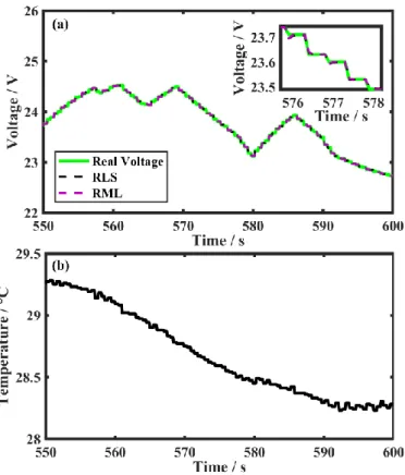
Figures 6 and 7 represent the estimated voltage and temperature variation for the Degraded and Normal PEMFCs respectively. As is clear in these figures, both of RLS and RML algorithms are potentially capable of estimating voltage precisely. It is difficult to form an opinion about the performance comparison of the algorithms solely by means of these figures.
Figure 6: Estimated output voltage (a), and temperature change (b), of the Degraded PEMFC.
Figure 7: Estimated output voltage (a), and temperature change (b), of the Normal PEMFC. Regarding the comparison of the algorithms to one another, the mean square error (MSE) and the peak signal to noise ratio (PSNR) have been employed. MSE and PSNR are two error
metrics used to compare the estimation quality. PSNR calculates the peak signal-to-noise ratio, in decibels, between the two original signal and estimated signal. In this paper, the original signal is the measured output voltage of the PEMFC and the estimated signal is the PEMFC estimated output voltage by the algorithms. The higher the PSNR, the better the quality of the estimation. The MSE represents the cumulative squared error between the
estimated voltage and the measured voltage. The lower the value of MSE, the lower the error. As mentioned earlier, the utilized algorithms in this work have been implemented in
LabVIEW software for experimental validation. The PEMFC is connected to a National Instrument CompactRIO, which provides access to the PEMFC voltage and temperature sensors’ measurements. In order to check the robustness of the algorithms, a random noise is added to the voltage measurement in the LabVIEW, and the noisy signal is sent to the process of identification, which is done by the algorithms. It should be reminded that the purpose of identification is to estimate output voltage of the PEMFC and that is why the noise is added to the voltage measurement. Figure 8 presents the obtained PSNR values for different cases. Four cases, namely zero noise, a random noise with variance of 0.25, a random noise with variance of 0.5, and a random noise with variance of 0.75, have been considered in this analysis. Zero noise refers to the normal measurement, and the other cases show the addition of random noise with different variances to test the robustness of the algorithms. As it is seen in Figure 8, in case of normal measured data (zero noise), RLS performs better than RML to some extent. However, as the level of noise increases RML algorithm indicates superior performance compared to RLS. This result implies that RML algorithm is more robust than RLS while confronting some noises in the system.
Figure 8: Comparison of the algorithms based on PSNR.
Figure 9 presents the comparison of the algorithms based on MSE metric for the same
discussed four cases. The achieved results of MSE analysis is in agreement with the results of PSNR, regarding the robustness of the algorithms. It is clear that the value of MSE for RLS is marginally lower that RML in normal measured data, and in higher noise levels, the MSE value of RML is lower than RLS, which shows its robustness against noise.
Figure 9: Comparison of the algorithms based on MSE.
Regarding the investigation of the result relevance to the physical meaning, current interrupt method, as explained in section 3.1, has been used to obtain a reference range for assessing the resistor estimation by algorithms. In fact, current interrupt test, which is an
electrochemical technique, is used to measure the evolution of resistor with respect to the temperature and current. This measurement clarifies the range of the resistor for the whole stack and is a helpful tool to check the achieved results by the both algorithms. Figure 10
within the obtained ranges of the current interrupt test presented in Figure 3. The observed evolution in the trend of resistor, particularly between 0 to 100 seconds, is due to the sharp rise of current in the used current profile, shown in Figure 5, in this time period. This sudden increase in the current also leads to a temperature rise, which affects the resistor. The resistor is influenced by not only the current but also the temperature. According to Figure 10, the ohmic resistance value in the Degraded PEMFC is more than the Normal PEMFC.
Figure 10: Evolution of the estimated ohmic resistance in the PEMFCs. Table 6 provides information on the average value of the semi-empirical parameters, obtained by both of the identification methods. There is not a lot of information about the range of the semi-empirical parameters in the literature and even in the few existing
manuscripts, there is not any explanation about the age and degradation level of the PEMFCs. However, the achieved parameters in this manuscript seem to be almost in the same range as in Table 2.
Table 6: The average obtained values of the semi-empirical parameters
Parameters Degraded PEMFC Normal PEMFC
RLS RML RLS RML ϒ1 -1.19 -1.19 -0.91 -0.91 ϒ2 4.01×10⁻³ 4.01×10⁻³ 2.9×10⁻³ 2.9×10⁻³ ϒ3 9.68×10⁻⁵ 9.53×10⁻⁵ 7.71×10⁻⁵ 7.78×10⁻⁵ ϒ4 -9.56×10⁻⁵ -1.05×10⁻⁴ -1.97×10⁻⁴ -1.93×10⁻⁴ α 7.95×10⁻¹ 7.95×10⁻¹ 9.94×10⁻¹ 9.94×10⁻¹ ξ1 9.94×10⁻² 9.94×10⁻² 1.07×10⁻² 1.07×10⁻² ξ2 -2.92×10⁻⁴ -2.92×10⁻⁴ -9.90×10⁻⁶ -1.00×10⁻⁵ ξ3 -1.22×10⁻⁵ -1.22×10⁻⁵ 8.54×10⁻⁵ 8.54×10⁻⁵
c1 - 2.50×10⁻¹ - 2.50×10⁻¹
c2 - 3.00×10⁻¹ - 3.00×10⁻¹
c3 - 5.00×10⁻² - 5.00×10⁻²
Figure 11 represents the evolution of the activation region parameters of the Normal PEMFC with RLS algorithm. Since the performance of the algorithms has been already discussed over the previous figures and the average values of the estimated parameters for both PEMFCs have been reported in Table 6, the parameters identified by RLS approach are only shown in Figure 11 to give an idea of parameters variation. As is seen in this figure, the parameters are time-varying and the small variation of the parameters overtime shows that the selected PEMFC model has an acceptable accuracy, otherwise the parameters would fluctuate a lot to compensate the lack of accuracy in the model.
Figure 11: The fluctuation of activation region parameters.
The variation of the concentration region parameter, achieved by RLS, is shown in Figure 12. It should be noted that the severity of degradation influence is ambiguous over each specific
parameter. However, it can be ensured that in case of disturbance occurrence due to degradation, the parameters change to embrace its effect.
Figure 12: The fluctuation of concentration region parameter.
Figure 13 represents the comparison of the polarization and power curves of Normal and Degraded PEMFCs with the estimated ones, obtained by RLS algorithm for zero noise condition. It should be noted that the polarization curve changes continuously mainly due to the temperature change. As it is seen, maximum power is achieved in the high current region, where the concentration part begins. In this regard, by employing the recursive algorithms in the parameter estimation of a PEMFC model, the polarization curve and maximum power can be obtained at each moment and be used in power splitting or global EMSs.
Figure 13: Polarization curve and corresponded power curve of Normal PEMFC (a, c), and Degraded PEMFC (b, d).
Figure 14 compares the polarization curves obtained by the estimated parameters with RML and RLS algorithms for the noise level of 0.25. As is clear in Figure 14, the estimated polarization curve by RML algorithm is closer to the reference, which comes from the
experimental data, than RLS. This figure also shows the influence of noise in the polarization curve estimation. Looking more closely at Figure 14, it can be concluded that a small change in the voltage estimation can cause a noticeable change in the polarization curve estimation. The difference between the PSNR values of RML and RLS algorithms, presented in Figure 8, for the noise level of 0.25 is not a lot. However, this slight difference causes an obvious change in the polarization curve prediction.
Figure 14: The comparison of polarization curves obtained by algorithms
6 Conclusions
This paper proposes online identification of a multi-input PEMFC model to track the performance drifts due to the influence of degradation phenomenon and the operating
conditions, which are not considered in the model, over the output voltage of a fuel cell system. In this regard, a semi-empirical PEMFC model is selected and two identification algorithms, RLS and RML, are utilized to update the chosen model. Various scenarios, four noise level cases, and two PEMFCs with different levels of degradation, have been considered to test the performance of the algorithms. The main results achieved from the experimental implementation and test of the algorithms indicate that both of the algorithms are capable of estimating the output voltage to a satisfactory level. However, RML has shown more
robustness in dealing with noisy measurement data. It is worth reminding that this robustness might lead to less expensive sensors and measurement instruments. Moreover, it should be noted that the range of alteration in the semi-empirical parameters was acceptable. In future, this work can be integrated into the design of global energy management for FCVs.
Acknowledgements
This work was supported by the Natural Sciences and Engineering Research Council of Canada (NSERC). This research was undertaken, in part, thanks to funding from the Canada Research Chairs program.
List of Symbols Latin Letters
VFC Output voltage of fuel cell / V
n Number of cells
ENernst Cell reversible voltage / V
Vact Activation voltage drop / V
Vohmic Ohmic voltage drop / V
Vcon Concentration voltage drop / V
T Stack temperature / K
PH2 Hydrogen partial pressure / Pa
PO2 Oxygen partial pressure / Pa
CO2 Oxygen concentration / molcm-3
i FC operating current / A
Rinternal Total internal resistance of the fuel cell / Ω
G Dimensionless number Y Output U Input V Noise an Output coefficient bm Input coefficient E Error cr Error coefficient k Kalman gain P Covariance matrix E Estimation error q-1 Delayed operator C Estimated polynomial X Regression vector I Identity matrix Greek Letters
ϒn Experiential coefficients related to activation loss
ξn Parametric coefficients related to ohmic resistance
Α Semi-empirical parameter related to diffusion mechanism
Β Inverse of the limiting current density / A-1cm-2
θ Parameter vector
Φ Linear regression vector
φ0 Residual regression vector
Λ Directional forgetting factor
Ε Residuals
Ψ Filter
Β Constant
Ω Forgetting factor
References
[1] U. Winter, H. Weidner, Fuel Cells 2003, 3, 76.
[2] C. Kompis, K. Malek, Fuel Cells 2016, 16, 760.
[3] N. Sulaiman, M. A. Hannan, A. Mohamed, E. H. Majlan, W. R. Wan Daud,
Renewable Sustainable Energy Rev. 2015, 52, 802.
[4] A. Panday, H. O. Bansal, Int. J. Veh. Technol. 2014, 2014, 1.
[5] S. F. Tie, C. W. Tan, Renewable Sustainable Energy Rev. 2013, 20, 82.
[6] O. Erdinc, M. Uzunoglu, Renewable Sustainable Energy Rev. 2010, 14, 2874.
[7] D. Zhou, A. Al-Durra, F. Gao, A. Ravey, I. Matraji, M. Godoy Simões, J. Power
Sources 2017, 366, 278.
[8] J. Chen, C. Xu, C. Wu, W. Xu, IEEE Trans. Ind. Inf. 2018, 14, 292.
[9] D. Zhou, A. Ravey, A. Al-Durra, F. Gao, Energy Convers. Manage. 2017, 151, 778.
[10] R. Koubaa, L. krichen, Energy 2017, 133, 1079.
[11] M. G. Carignano, R. Costa-Castelló, V. Roda, N. M. Nigro, S. Junco, D. Feroldi, J.
[12] L. Xu, J. Li, M. Ouyang, Int. J. Hydrogen Energy 2015, 40, 15052.
[13] J. Bernard, S. Delprat, T. M. Guerra, F. N. Büchi, Control Eng. Pract. 2010, 18, 408.
[14] D. Feroldi, M. Serra, J. Riera, J. Power Sources 2009, 190, 387.
[15] A. A. Shah, K. H. Luo, T. R. Ralph, F. C. Walsh, Electrochim. Acta 2011, 56, 3731.
[16] M. Eikerling, Fuel Cells 2016, 16, 663.
[17] M. Karimi, J. Yahyazadeh, A. Rezazade, Fuel Cells 2016, 16, 530.
[18] K. Ou, Y. X. Wang, Y. B. Kim, Fuel Cells 2017, 17, 299.
[19] P. Xu, S. Xu, Fuel Cells 2017, 17, 794.
[20] N. Bizon, Appl. Energy 2013, 104, 326.
[21] Z.-d. Zhong, H.-b. Huo, X.-j. Zhu, G.-y. Cao, Y. Ren, J. Power Sources 2008, 176,
259.
[22] F. X. Chen, Y. Yu, J. X. Chen, Fuel Cells 2017, 17, 671.
[23] A. Harrag, S. Messalti, Fuel Cells 2017, 17, 816.
[24] K. Ettihir, L. Boulon, K. Agbossou, 5th International Conference on Fundamentals &
Development of Fuel Cells (FDFC 2013), 2013.
[25] K. Ettihir, L. Boulon, K. Agbossou, IET Electr. Syst. Transp. 2016, 6, 261.
[26] K. Ettihir, L. Boulon, K. Agbossou, Appl. Energy 2016, 163, 142.
[27] K. Ettihir, L. Boulon, M. Becherif, K. Agbossou, H. S. Ramadan, Int. J. Hydrogen
Energy 2014, 39, 21165.
[28] S. Kelouwani, N. Henao, K. Agbossou, Y. Dube, L. Boulon, IEEE Trans. Veh.
Technol. 2012, 61, 3851.
[29] R. N. Methekar, S. C. Patwardhan, R. D. Gudi, V. Prasad, J. Process Control 2010, 20,
73.
[30] D. Li, Y. Yu, Q. Jin, Z. Gao, Energy 2014, 68, 210.
[31] L. Xu, J. Li, J. Hua, X. Li, M. Ouyang, J. Power Sources 2009, 194, 360.
[32] L. Pisani, G. Murgia, M. Valentini, B. D’Aguanno, J. Power Sources 2002, 108, 192.
[33] R. F. Mann, J. C. Amphlett, M. A. I. Hooper, H. M. Jensen, B. A. Peppley, P. R.
Roberge, J. Power Sources 2000, 86, 173.
[34] J. C. Amphlett, R. M. Baumert, R. F. Mann, B. A. Peppley, P. R. Roberge, T. J.
Harris, J. Electrochem. Soc. 1995, 142, 9.
[35] M. Ali, M. A. Elhameed, M. A. Farahat, Renewable Energy 2017, 111, 455.
[36] O. E. Turgut, M. T. Coban, Ain Shams Eng. J. 2016, 7, 347.
[37] Z. Sun, N. Wang, Y. Bi, D. Srinivasan, Energy 2015, 90, 1334.
[38] C. Restrepo, T. Konjedic, A. Garces, J. Calvente, R. Giral, IEEE Trans. Ind. Inf. 2015,
11, 548.
[39] K. Priya, T. Sudhakar Babu, K. Balasubramanian, K. Sathish Kumar, N. Rajasekar,
Sustainable Energy Technol. Assess. 2015, 12, 46.
[40] G. Squadrito, G. Maggio, E. Passalacqua, F. Lufrano, A. Patti, J. Appl. Electrochem.
1999, 29, 1449.
[41] A. Husar, S. Strahl, J. Riera, Int. J. Hydrogen Energy 2012, 37, 7309.
[42] J. Wu, X. Yuan, H. Wang, M. Blanco, J. Martin, J. Zhang, Int. J. Hydrogen Energy
2008, 33, 1735.
[43] K. R. Cooper, M. Smith, J. Power Sources 2006, 160, 1088.
[44] T. Mennola, M. Mikkola, M. Noponen, T. Hottinen, P. Lund, J. Power Sources 2002,
112, 261.
[45] R. Isermann, Automatica 1980, 16, 575.
[46] L. Cao, H. Schwartz, Automatica 2000, 36, 1725.
[47] C. Depature, S. Jemei, L. Boulon, A. Bouscayrol, N. Marx, S. Morando, A. Castaings,
IEEE Vehicle Power and Propulsion Conference (VPPC), Hangzhou, 2016, IEEE, pp. 1.