1
Demand Driven Dispatch and Revenue Management
byDaniel G. Fry
B.A. Economics and Mathematics, Augustana College (SD), 2013
Submitted to the Department of Civil and Environmental Engineering in partial fulfillment of the requirements of the degree of
Master of Science in Transportation
at the
MASSACHUSETTS INSTITUTE OF TECHNOLOGY
June 2015
© 2015 Massachusetts Institute of Technology. All rights reserved.
Author ... Department of Civil and Environmental Engineering
May 8, 2015
Certified by ... Peter. P. Belobaba Principal Research Scientist of Aeronautics and Astronautics Thesis Supervisor
Accepted by ... Heidi Nepf Donald and Martha Harleman Professor of Civil and Environmental Engineering Chair, Graduate Program Committee
2
Demand Driven Dispatch and Revenue Management
byDaniel G. Fry
Submitted to the Department of Civil and Environmental Engineering on May 8, 2015 in partial fulfillment of the requirements of the degree of Master of Science in Transportation ABSTRACT
The focus of this thesis is on the integration of and interplay between demand driven patch and revenue management in a competitive airline network environment. Demand driven dis-patch is the reassignment of aircraft to flights close to departure to improve operating profitability. Previous studies on demand driven dispatch have not incorporated competition and have typically ignored or significantly simplified revenue management. All simulations in this thesis use the PODS simulator, where stochastic demand by market chooses between competing airlines with alternative paths and fare products whose availability is determined by industry-typical revenue management systems.
Demand driven dispatch (D³) is tested with a variety of methods and objectives, including a bookings-based method that assigns the largest aircraft to the flights with the highest forecasted demands. More sophisticated methods include revenue- and profit-maximizing fleet optimizations that directly use the output of leg-based and network-based RM systems and a minimum-cost flow specification. D³ is then tested with a variety of aircraft swap timings, RM systems, and competitive scenarios. Sensitivity testing is performed at a variety of demand levels, demand variability levels, and with an optimized static fleet assignment. Findings include important competitive feedbacks from D³, relationships between D³ and both revenue management and pricing, and important nu-ances to D³’s relationship with the level and variability of demand.
Depending on how it is implemented, D³ may harm competitor airlines more than it aids the implementer. Early swaps in D³ lead to heavy dilution. Late swaps lead to smaller increases in loads but substantial increases in revenue. The relationship between revenue-maximization and cost-minimization in profit-maximizing D³ is highly influenced by the timing of swaps, revenue estima-tion, and demand levels. Finally, early swaps are susceptible to high variability of demand while late swaps are more robust. Findings indicate that the benefits of D³ can be estimated at operating profit gains of 0.04% to 2.03%, revenue gains of 0.02% to 0.88%, and changes in operating costs of -0.08% to 0.13%.
Thesis Supervisor: Peter P. Belobaba
3
Acknowledgements
First and foremost, I would like to thank my advisor Dr. Peter Belobaba. He has offered invaluable support, guidance, and knowledge over the last two years for which I am incredibly thankful. It has truly been a pleasure to take his courses, research with him, and more than occasionally exchange airline banter. His help has been instrumental in my suc-cess at MIT and I cannot thank him enough.
I would also like to thank Craig Hopperstad and Matthew Berge for their help in designing the D³ assignment process and coding it into PODS. The simulation went from ad hoc capacity changes without constraints to a fully functioning fleet assignment optimi-zation, and it is due to Craig and Matthew. Thank you for making my research possible.
I thank Kirsten Amrine, Jimmy Chang, and Scott Suttmeier for the excellent intern-ship with Alaska Airlines. Not only did I have a great time, I learned a great deal about the airline planning process in practice and got to see my research become reality in the Alaska network. That has certainly contributed to the quality of my research this year.
I would also like to thank Mike, Eric, Karim, and Yingzhen. It was a real pleasure to work with them the first year; they helped me feel at home in Boston. Mike and Eric were also great teachers. And thank you Tamas: I really enjoyed the plane spotting trips. It’s great to have great friends.
Thank you to this year’s first years: Oren, Germán, Adam, Alex, and Henry. You’ve been a lot of fun to work with and to get to know, and I’ve enjoyed talking with you about RM, the airline industry, and stories of South Dakota. Again, it’s great to have great friends Last, but certainly not least, I have to thank my family and my friends from beyond MIT. You know who you are, especially if you’ve been spending hours on skype or the phone lending advice, jokes, and general morale. I’ve probably talked to you about my research so much by now you might think you’ve written a thesis. Anyhow, your conversa-tion, your visits, and your unfailing support are tremendous. Thank you.
4
Table of Contents
Table of Figures ... 6
Table of Tables ... 9
Chapter 1: Introduction ... 10
1.1. Variability in Airline Demand ... 11
1.2. Current Planning and RM Process and Demand Driven Dispatch... 12
1.3. Motivation for Research ... 13
1.4. Outline of Thesis ... 14
Chapter 2: Background & Literature Review ... 16
2.1. Network Planning, Scheduling, and Pricing ... 16
2.2. Revenue Management ... 20
2.2.1. Forecasting ... 23
2.2.2. Optimization ... 26
2.3. Airline Demand: RM, Spill, and Incremental Capacity ... 27
2.4. Previous Research in D³... 28
Chapter 3: About PODS ... 32
3.1. Overview and Structure ... 32
3.2. Competitive Networks... 34
3.3. Demand Generation and Passenger Choice ... 35
3.4. Modeling Demand Driven Dispatch in PODS ... 37
3.5. PODS Network D³ ... 37
Chapter 4: Bookings-Based Swapping ... 44
4.1. Swapping Methodology ... 44
4.2. Dimensions of D³ Experiments ... 46
4.2.1 Timing Swaps ... 47
4.2.2. Swaps with Different RM Systems & Competition ... 56
4.2.3. Demand Level Effects ... 67
4.3. Conclusions from Bookings-Based D³ ... 71
Chapter 5: Network Optimization Fleet Assignment ... 73
5.1. The Network Optimizer ... 73
5
5.1.2. Modeling Assumptions ... 76
5.2. Revenue Estimation ... 78
5.2.1. Estimating Revenue with EMSRb ... 78
5.2.2. Estimating Revenue with DAVN and Other OD Techniques ... 80
5.3. Cost Estimation ... 81
5.4. The Experiments ... 83
Chapter 6: D³ with Optimized Swapping ... 85
6.1. Timing the Swaps ... 85
6.1.1. Timing Swaps with Leg-Based RM ... 86
6.1.2. Timing Swaps with DAVN ... 97
6.2. Competitive Demand Driven Dispatch ... 107
6.2.1. Competitive D³ at Time Frame 6 ... 109
6.2.2. Competitive D³ at Time Frame 14 ... 112
6.2.3. Asymmetric Competitive D³ ... 115
6.3. Conclusions from Optimized Swapping ... 119
7. Chapter 7: Sensitivity Analysis... 121
7.1. Varying Demand Levels ... 121
7.2. Optimizing Airline 1’s Fleet Assignment ... 128
7.3. D³ with Demand Variability and the New Fleet Assignment ... 133
8. Chapter 8: Conclusions ... 140
8.1. A Review of Demand Driven Dispatch ... 140
8.2. Insights from Bookings-Based Swapping ... 141
8.3. Insights from Optimized Swapping ... 143
8.4. Insights from Sensitivity Testing ... 145
8.5. Suggestions for Future Research... 146
Bibliography ... 149
6
Table of Figures
Figure 1: Demand Segmentation ... 19
Figure 2: Serial Nesting ... 22
Figure 3: Structure of PODS ... 33
Figure 4: TF Definitions ... 34
Figure 5: Demand Arrival ... 36
Figure 6: Network D³ Markets ... 38
Figure 7: Airline 1 Route Map ... 39
Figure 8: Airline 2 Route Map ... 39
Figure 9: Flight String Design ... 39
Figure 10: Routing Options ... 40
Figure 11: Network D³ Fare Restrictions ... 41
Figure 12: Network D³ Fare Structures ... 43
Figure 13: Bookings-Based Assignment Example ... 45
Figure 14: Example of Suboptimal Assignment ... 46
Figure 15: Swap Times ... 48
Figure 16: Changes in System Revenue from Bookings-Based D³ at Different TFs ... 49
Figure 17: Changes in RPMs from Bookings-Based D³ at Different TFs ... 50
Figure 18: Changes in ASMs from Bookings-Based D³ at Different TFs ... 50
Figure 19: Changes in System LF Points from Bookings-Based D³ at Different TFs ... 51
Figure 20: Changes in Yield from Bookings-Based D³ at Different TFs ... 51
Figure 21: Percentage of Swapped Leg-Pairs in Swappable Set, Bookings-Based D³ at Different TFs ... 52
Figure 22: Magnitudes of Booking Changes from Bookings-Based D³ at Different TFs ... 53
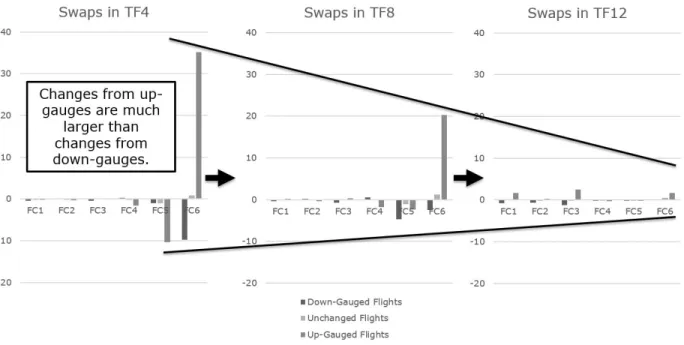
Figure 23: Changes in Gauge vs. Changes in Bookings ... 54
Figure 24: Timing Effects in Bookings from Bookings-Based D³ at Different TFs ... 55
Figure 25: Changes in Bookings after 21-Day AP, Bookings-Based D³ ... 56
Figure 26: EMSRb, Airline 1 Uses Bookings-Based D³ ... 57
Figure 27: EMSRb, Airline 2 Uses Bookings-Based D³ ... 58
Figure 28: EMSRb, Both Airlines Use Bookings-Based D³ ... 58
Figure 29: DAVN, Airline 1 Uses Bookings-Based D³ ... 60
Figure 30: DAVN, Airline 2 Uses Bookings-Based D³ ... 60
Figure 31: DAVN, Both Airlines Use Bookings-Based D³ ... 61
Figure 32: ProBP, Airline 1 Uses Bookings-Based D³ ... 62
Figure 33: ProBP, Airline 2 Uses Bookings-Based D³ ... 62
Figure 34: ProBP, Both Airlines Use Bookings-Based D³ ... 63
7
Figure 36: DAVN w/ HF/FA, Airline 2 Uses Bookings-Based D³ ... 64
Figure 37: DAVN w/ HF/FA, Both Airlines Use Bookings-Based D³... 64
Figure 38: Airline 1 Implements D³, LF & Yield Figure 39: Airline 2 Implements D³, LF & Yield... 65
Figure 40: Both Airlines Implement D³, LF & Yield ... 66
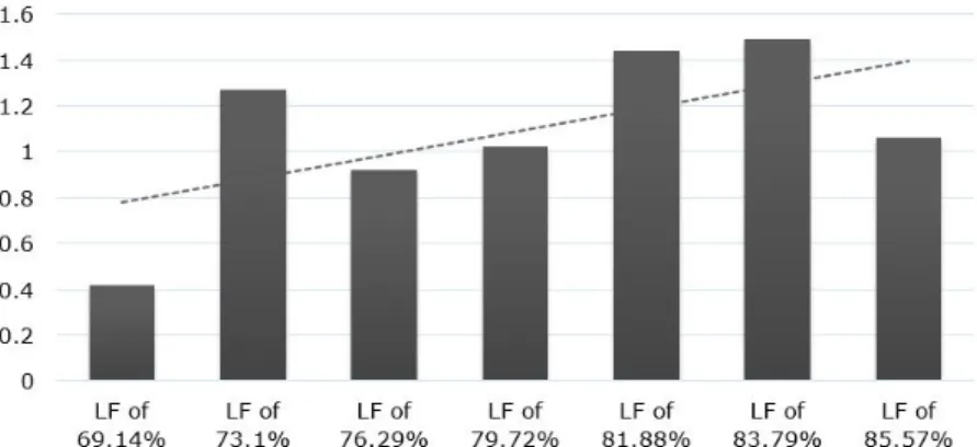
Figure 41: Base Case System Load Factors for Seven Demand Levels ... 67
Figure 42: Revenue Changes from Bookings-Based D³ at Different Demands ... 68
Figure 43: LF % pt. Changes from Bookings-Based D³ at Different Demands ... 69
Figure 44: Changes in ASMs and RPMs from Bookings-Based D³ at Different Demands ... 69
Figure 45: Changes in Yield from Bookings-Based D³ at Different Demands ... 70
Figure 46: % of Swapped Leg-Pairs in the Swappable Set, Bookings-Based D³ at Different Demands ... 70
Figure 47: Average Differences of Initial Capacity and Forecasted BAD ... 71
Figure 48: Example of Min-Cost Flow Specification (by Matthew Berge) ... 74
Figure 49: EMSR Hull for EMSRb ... 79
Figure 50: Times of the Optimized Swaps ... 86
Figure 51: Changes in Operating Profit, Optimized D³ with EMSRb ... 88
Figure 52: Changes in Revenue, Optimized D³ with EMSRb ... 89
Figure 53: Changes in Op. Costs and ASMs, Optimized D³ with EMSRb ... 91
Figure 54: Changes in RPMs, Optimized D³ with EMSRb ... 92
Figure 55: Changes in LF % pts, Optimized D with EMSRb ... 93
Figure 56: Changes in Yield, Optimized D³ with EMSRb ... 94
Figure 57: Changes in Bookings by FC, Optimized D³ with EMSRb at TF 6 ... 95
Figure 58: Changes in Bookings by FC, Optimized D³ with EMSRb at TF14 ... 96
Figure 59: Changes in Operating Profit, Optimized D³ with DAVN ... 98
Figure 60: Changes in Revenue, Optimized D³ with DAVN ... 99
Figure 61: Changes in Op. Costs and ASMs, Optimized D³ with DAVN ... 100
Figure 62: Changes in RPMs, Optimized D³ with DAVN ... 101
Figure 63: Changes in LF % pts, Optimized D³ with DAVN... 101
Figure 64: Changes in Yield, Optimized D³ with DAVN ... 102
Figure 65: Changes in Bookings by FC, Optimized D³ with DAVN at TF6 ... 103
Figure 66: Changes in Bookings by FC, Optimized D³ with DAVN at TF14 ... 103
Figure 67: Change in DCs in Top Quartile of Fullest Flights from D³ at TF14 ... 104
Figure 68: Change in DCs in Third Quartile of Fullest Flights from D³ at TF14 ... 105
Figure 69: Changes in Forecasted BTC for FC1 with D³ at TF14 ... 106
Figure 70: Changes in LF % pts with Competitive D³ ... 108
Figure 71: Changes in ASMs, RPMs, and Yield When D³ is Implemented at TF6 ... 110
8
Figure 73: Changes in ASMs, RPMs, and Yield When D³ is Implemented at TF14 ... 113
Figure 74: Changes in Revenue, Op. Costs, and Op. Profit When D³ is Implemented at TF14 .. 114
Figure 75: Changes in ASMs, RPMs, and Yield When D³ is Implemented Asymmetrically ... 116
Figure 76: Changes in Rev., Op. Costs, and Op. Profits When D³ is Implemented Asymmetrically ... 117
Figure 77: Game Theory Grid of Op. Profit Outcomes from D³ ... 118
Figure 78: Airline 1 Base Case Load Factors for Sensitivity Analysis ... 122
Figure 79: LF Distributions for Highest and Lowest Demand Levels ... 123
Figure 80: % of Swappable Flights Swapped from D³, Varying Demand Levels ... 124
Figure 81: Changes in ASMs and RPMs from D³, Varying Demand Levels ... 125
Figure 82: Changes in LF %pts and Yield from D³, Varying Demand Levels ... 126
Figure 83: Changes in Revenue, Op. Costs, and Op. Profits from D³, Varying Demand Levels .. 127
Figure 84: Changes in Revenue, Op. Costs, and Op. Profit from D³ at TF6 with Different K-Factors ... 134
Figure 85: Changes in ASMs and RPMs from D³ at TF6 with Different K-Factors ... 135
Figure 86: Changes in Revenue, Op. Costs, and Op. Profit from D³ at TF14 with Different K-Factors ... 137
Figure 87: Changes in LF %pts and Yield from D³ at TF14 with Different K-Factors ... 138
Figure 88: Changes in ASMs and RPMs from D³ at TF14 with Different K-Factors ... 138
Figure 91: ProBP w/ HF/FA, Airline 1 Uses Bookings-Based D³ ... 153
Figure 92: ProBP w/ HF/FA, Airline 2 Uses Bookings-Based D³ ... 153
Figure 93: ProBP w/ HF/FA, Both Airlines Use Bookings-Based D³ ... 153
Figure 94: Changes in ASMs, RPMs and Yield, AL1 w/ D³ at TF14, AL2 at TF6 ... 154
9
Table of Tables
Table 1: Network D³ Fare Structures ... 42
Table 2: Base Case Output with EMSRb ... 47
Table 3: Block Hour Costs by Capacity ... 82
Table 4: Base Case Profit Results ... 83
Table 5: Percentage of Swappable Flights that Experienced Swaps, EMSRb ... 88
Table 6: Percentage of Swappable Flights that Experienced Swaps, DAVN ... 98
Table 7: % Chg. in Forecasted BTC in TF1 by FC, from D³ in TF14... 106
Table 8: Most Common Aircraft Assignments, D³ in TF2 with DAVN ... 129
Table 9: Primary Base Results with Original Static Fleet Assignment ... 131
Table 10: Primary Base Results with Optimized Static Fleet Assignment ... 131
Table 11: Changes in Primary Results from Optimizing Static Fleet Assignment ... 131
Table 12: Changes in Primary Results from D³ at TF6, Given the Optimized Static Fleet Assignment ... 132
Table 13: Changes in AL1 Revenue, TF Summary, Bookings-Based Swapping ... 141
Table 14: Changes in AL1 Revenue, Demand Level Summary, Bookings-Based Swapping ... 142
Table 15: Changes in AL1 Profit, TF Summary, Optimized Swapping ... 144
10
Chapter 1: Introduction
The planning process of an airline can be thought of as a series of decisions first at a strategic level and then at a tactical level as the departure date draws closer (Belobaba, 2009b). Generally, airlines begin with fleet planning, then route planning, and then schedule development. Fleet planning can take place many months to many years in advance, route planning on a closer time horizon, and schedule development usually six or more months from departure. Schedule development involves first frequency planning, then timetable development, and finally fleet assignment, where aircraft types are assigned to specific flights. At this point, crew and maintenance schedules can be determined and more tactical decisions take over—namely pricing and revenue management. Due to this linear chronology in the airline planning process, aircraft schedules and therefore capacity on every flight is effectively fixed for pricing and revenue management, with exceptions for unplanned capac-ity changes. These changes in capaccapac-ity are then viewed from the perspective of pricing and revenue management as capacity disturbances.
Demand driven dispatch swaps aircraft of different sizes on flight legs to change capacity in response to demand. With schedules having been made perhaps six or more months ahead of the departure date, pricing and revenue management then operate with the assumption of fixed capacity to maximize revenue. Demand driven dispatch makes ca-pacity flexible again, changing aircraft assignments nearer to departure, often called close-in refleetclose-ing. Thus, usclose-ing more detailed and reliable demand close-information from the revenue management system, demand driven dispatch has the potential to better match capacity supplied with quantity demanded, simultaneously increasing revenues and decreasing oper-ating costs (Berge & Hopperstad, 1993).
Theoretically promising, demand driven dispatch still poses a host of challenges, including not only potential disruptions to already complicated aircraft, crew, and mainte-nance schedules, but also a significant interaction with the revenue management process. Revenue management, as it is practiced, assumes a fixed capacity on each flight and opti-mizes fare class inventory accordingly; to date, the interaction of revenue management and demand driven dispatch in a competitive network environment has not been explored. Fur-thermore, attention has not been paid to incorporating the full wealth of information pro-vided by revenue management into the fleet assignment process of demand driven dispatch.
Therefore, while demand driven dispatch is a step towards a successful integration of scheduling and revenue management, a good deal is left to do before the integration is truly complete. Both the type of information gathered from the revenue management system
11
and how that information is put to use in fleet assignment can be better informed by the theory and application of subsequent inventory control. Second, demand driven dispatch must be analyzed in a competitive network environment. The aim of this thesis is to address these points and develop a better understanding of the impact demand driven dispatch has on the revenue and profit results of airline operations, with a particular focus on demand driven dispatch given both a competitive environment and the range of typical practices in revenue management.
1.1. Variability in Airline Demand
Variability in airline demand is a well-documented phenomenon. Demand for air travel varies by season, holidays and sporting events, day of week, time of day, the macro-economy, security threats, weather, and countless other factors. From the perspective of a single airline, variations in realized demand are affected by relative fares and fare class availability, revenue management practices, competing schedules and routings from not only other carriers’ itineraries but their own as well.
Yet, nearly every facet of the airline planning process relies on forecasts of demand for flight legs or paths, from network planning, scheduling and fleeting to pricing and reve-nue management. Operations research has had some of its most notable applications in the airline industry, but operations research results in optimal outcomes only when its assump-tions and inputs, largely forecasts, are correct. Therefore, the best possible forecasts in terms of accuracy are needed. As accuracy is lacking due to variability in demand, it is also important that the systems that use these forecasts are built robustly. Demand driven dis-patch is one approach to addressing variability of demand and making the planning process more flexible, and therefore more robust. It is not as critical that the forecast that informs the original schedule and fleet assignment be accurate if the fleet assignment can be updated at a later date with presumably better forecasts.
One of the key forecast strengths of using forecasts from revenue management is that they are made relatively close to the departure date. Uncertainty diminishes in expected demand both as the forecasts are generated closer to a flight’s departure date and of course as actual bookings are taken. With the notable exception of no-shows and cancellations, bookings that have already been taken are effectively deterministic demand. The original fleet assignment constrains future changes in capacity based on swapping options and crew constraints, etc., so that the original schedule and fleet assignment is certainly important. However, the ability to draw on improved forecasts from the RM system closer to departure
12
allows an airline to manage variability in demand by making adjustments to the fleet as-signment.
1.2. Current Planning and RM Process and Demand Driven Dispatch
The future of airline planning looks toward the integration of the different steps in the planning process. As is widely recognized, fleet planning depends on what routes an airline intends to fly, the profitability of routes not only depends on the available fleet but also the intended frequencies, and timetables rely on frequency plans but can also be tweaked to help optimize fleet assignment. Finally, the fleet assignment process relies on the selected timetables but also on pricing and revenue management practices such as will-ingness-to-pay forecasting and optimization.
Therefore, the different aspects of airline planning are interdependent and a true optimization of the whole “problem” of airline planning would have to be simultaneous— an impossible task in practice. What is much more attainable is the partial integration of components of the process. Each stage of optimization in the airline planning process con-strains the solutions of the next processes, but increasing the connections between the dis-parate processes theoretically loosens the constraints put on subsequent optimizations. Demand driven dispatch is primarily an attempt to integrate some components of schedul-ing, namely fleet assignment, with revenue management.
However, demand driven dispatch incorporates not only scheduling, or more precisely fleet assignment, and revenue management, it also affects and depends on all stages of the planning process. Fleet planning is essential to demand driven dispatch as both labor agree-ments and industry regulation effectively allow only aircraft of the same “family” to swap flight assignments. Therefore it is important that the fleet contains multiple aircraft types of different sizes within the same family so that pilots can exploit cockpit commonality. Network planning is also important, as the architecture of the network determines both the ease of performing aircraft swaps (altering the fleet assignment) but also the number of feasible swaps at any given airport at any given time. Hub networks offer excellent oppor-tunities for demand driven dispatch, while point-to-point networks do not disallow it but offer fewer swap opportunities.
Meanwhile, demand driven dispatch can better inform all of these aspects of airline planning. The ability to manage variability in demand with demand driven dispatch can allow airlines to strategically deploy larger aircraft to only high demand flights while the fleet at large is composed of mainly smaller aircraft, thus saving operating and ownership
13
costs (Berge & Hopperstad, 1993). The goal of an airline to engage in demand driven dis-patch may also inform an airline’s decision to consolidate its fleet into swappable aircraft families, along with a host of other noted efficiencies gained from streamlined fleet compo-sition. The ability to perform simplified demand driven dispatch can also be yet another factor in a long list that supports the recurring use of hub-and-spoke network design in the airline industry. On the other hand, demand driven dispatch can result in dilution that harms revenue performance. Pricing may have to adapt fare structures where possible to address this problem.
Demand driven dispatch is primarily an integration of components of scheduling and revenue management, but it effects and depends on all aspects of the planning process to some degree. The current airline planning process is often linear, with each decision process constrained by the decisions made before, and often by separate departments within an airline. Demand driven dispatch is a step towards breaking the information silos that come from such a process and, by increasing communication between fleet assignment and reve-nue management, can improve performance outcomes in operating profit by both increasing revenues and decreasing operating costs.
1.3. Motivation for Research
Demand driven dispatch thus far has largely been explored and tested as a process of taking demand forecasts from the revenue management system to repeat the fleet assign-ment process automatically or manually closer to departure. The act of using demand fore-casts from the revenue management (RM) system in the place of more aggregate forefore-casts to reassign aircraft is a likely improvement and accurately called close-in refleeting by some airlines. It does not, however, signify the successful or complete integration of revenue man-agement and fleet assignment.
This thesis aims to develop a more thorough understanding of demand driven dis-patch by focusing on the revenue management portion of demand driven disdis-patch, an area that has been somewhat neglected in previous studies. Revenue management systems can provide information to the fleet assignment model (FAM) beyond more accurate demand forecasts such as demand by fare class with network revenue values. Demand driven dis-patch is simulated for this thesis using the Passenger Origin Destination Simulator (PODS), so that demand driven dispatch and its effects can be analyzed in a network setting with complete RM systems and competition, a very important factor. The airline industry is highly competitive and passengers are both price-sensitive and have at their disposal unri-valed information when searching for the lowest fares. Demand driven dispatch must be
14
considered in the context of competition, and it should also utilize the full body of infor-mation provided by RM and RM in turn should be informed in some fashion of capacity changes made by demand driven dispatch. Therefore, the primary contribution of this thesis is to analyze demand driven dispatch in the context of two competing network airlines using complete revenue management systems.
These revenue management systems, depending on their complexity, can supply a host of information to the fleet assignment process beyond a count of passenger demand and average selling fare. First and foremost, RM forecasts divides demand into inventory fare classes, each with its own associated fare value(s). Through effective inventory control, RM also applies a hierarchy of fare classes so that when making fleet assignment decisions with RM forecasts, it is possible to evaluate the marginal revenue value of each additional seat or block of seats on a particular flight. This detail is important, as the use of RM means that the additional revenue value of the “last” seat on a flight is necessarily less than the average selling fare. RM methods that consider the network revenue value of fare class inventory can also provide information on the revenue value of capacity on a flight not only to that flight but also to the network as a whole. Thus, the fleet assignment component of demand driven dispatch can incorporate some degree of the revenue management’s infor-mation of network value to the fleet assignment decision. These opportunities to improve demand driven dispatch have not been fully explored.
Thus, the motivation for this thesis is to advance the science behind both revenue management and fleet assignment by developing a more thorough understanding of and several models for better integrating the two in demand driven dispatch (D³), especially with regard to RM’s role in informing D³, how it can be adapted to D³, and how it affects the outcome of D³. These areas, to date, have not been thoroughly addressed. This thesis is also motivated by the opportunity to simulate and analyze D³ with these innovations in a competitive network environment, something that has never been done. Thus, while ex-isting research in demand driven dispatch promises increased operating efficiency and im-proved profitability for airlines, many avenues for continued research remain.
1.4. Outline of Thesis
The thesis begins with this introduction and then proceeds to a more thorough review of the background of demand driven dispatch with a literature review of pertinent topics (Chapter 2), most notably in demand driven dispatch itself but also revenue management, fleet assignment, and other topics. The different forms of revenue management systems used
15
in this thesis will be reviewed in Section 2.2. Chapter 3 contains an overview of the Passen-ger Origin Destination Simulator (PODS) used to simulate demand driven dispatch for this thesis. This chapter contains details of its passenger demand components and its revenue management system components, which allow PODS to simulate imperfect knowledge of demand from the perspective of the airlines. The demand assumptions in PODS are also different from demand assumptions used in previous D³ research in that demand for differ-ent fare classes is not independdiffer-ent. Passengers are generated with preferences and willing-ness to pay and then choose the itineraries that best match their preferences and budget. PODS also incorporates competition, an important contribution to the literature on D³. The chapter also contains a description of Network D³, a hypothetical airline network spe-cifically designed and constructed for simulating demand driven dispatch in PODS.
The subsequent Chapters 4 through 7 detail the results of tests of demand driven dispatch in PODS. First, bookings-based swapping is evaluated in Chapter 4 with a simple ranking algorithm. This is to simulate the simplest form of demand driven dispatch and to form a basis for which to judge the value of more complicated demand driven dispatch techniques incorporating more information from RM. The ranking algorithm is replaced with an assigner built on a network optimization (minimum-cost flow model) in Chapter 5. This assigner is then used with a series of revenue-maximizing objective functions, starting with leg-based revenue estimation and RM optimization and culminating in the use of net-work bid prices. Finally, operating costs are also added to the objective function, which in turn maximizes operating profits. The results of tests using this assigner are shown in Chap-ter 6.
Chapter 7 presents the results of tests where demand driven dispatch is implemented for operating profit maximization under a wider range of conditions. A new static fleet assignment is introduced to test the benefits of D³ given an optimized original fleet assign-ment. Then, variation in demand is increased and decreased to test D³ benefits depending on variation in demand. Finally, the direct cost of aircraft swapping is tested at various levels. The thesis then concludes in Chapter 8 with a summary of results and concepts and suggestions for future research.
16
Chapter 2: Background & Literature Review
This chapter reviews the general trends in the science of airline planning over the last few decades, as well as describe current planning processes at airlines. The chapter begins with a discussion of network planning, scheduling and fleet assignment, and then pricing. These processes usually occur sequentially and typically precede revenue manage-ment and demand driven dispatch, should it be implemanage-mented. However, the approach used in these planning stages can limit or facilitate revenue management and demand driven dispatch.
Following the description of network planning, scheduling, and pricing, revenue man-agement is discussed, including current practices and near-future developments. The reve-nue management section is divided into two sections—forecasting and optimization. Numerous approaches to forecasting and optimization are used in the industry, with the most recent developments being focused on forecasting and optimizing demand by willing-ness-to-pay rather than strictly by fare class.
The interaction between revenue management and spill (rejected demand) is dis-cussed along with the modeling of spilled revenue. This section is brief but very pertinent to demand driven dispatch, as revenue management ultimately affects which types of de-mand are spilled and which are not.
Finally, Section 2.4 reviews the existing literature on demand driven dispatch. D³ debuted in academic journals in 1993 and has been researched since. The existing research primarily developed algorithms for modifying the fleet assignment problem to meet the specific constraints of demand driven dispatch. Competition among is not considered, nor is revenue management considered beyond simple representations of RM systems and de-mand arrival processes. However, impressive work has been completed on assignment algo-rithms, and analyses of live tests have also been conducted.
2.1. Network Planning, Scheduling, and Pricing
Network planning, also known as route planning, is in some regards the beginning of the planning process for deciding how to deploy an airline’s available fleet. Network plan-ning not only includes the process of deciding what origin and destination markets (OD markets) an airline will provide transportation between, but how that transportation net-work will be constructed. The most obvious decision in the architecture of a netnet-work is whether to deploy aircraft point-to-point or in a hub-and-spoke system. Point-to-point sys-tems offer convenient service to individual passengers, as they do not have to connect. On
17
the other hand, with no connecting passengers on point-to-point flights, limited demand may result in few frequencies or no service at all. From the perspective of airlines, hubs have undeniable benefits from operational efficiencies in fleet assignment to crew and per-sonnel scheduling. Most notably however, they allow airlines to use fewer aircraft and fewer flights to offer service to more destinations from any given origin in the hub-and-spoke network (Belobaba, 2009b).
Hub-and-spoke-systems also have economic costs related to their operations, such as decreased aircraft utilization in order to time arrivals and connecting departures from a hub, congestion at the hub airports, and extended turnaround times to allow passengers to connect. The growth of low cost carriers has caused some to forecast more point-to-point service, a trademark of the low-cost carrier model. However, with weaker demand post-2001 and 2008 and, until very recently, high fuel prices, hubs have been strengthened in recent years (Belobaba, 2009b). In fact, many airlines considered to be low-cost carriers utilize, if not hubs, focus cities. The term “hub” is difficult to define, but Southwest Airlines connects large numbers of passengers through several airports such as Midway in Chicago, and Jet-Blue does the same at airports such as JFK. In fact, many low-cost carriers, if they don’t have outright “hubs,” have significant focus cities, as found in an analysis of European low-cost carriers (Dobruszkes, 2006).
This observation is critical for demand driven dispatch, as wherever and whenever two or more aircraft of an airline have turns at an airport at overlapping times, the possi-bility for swapping exists. Thus, demand driven dispatch is possible for even dispersed point-to-point networks so long as aircraft occasionally “meet” in the network. However, hub-and-spoke networks provide for many more swapping opportunities, especially when aircraft are routed “to and from” hubs in short strings of flights. This fact has been recognized both in the literature and by airlines that have engaged in demand driven dispatch (Waldman, 1993). The practicality of demand driven dispatch, especially concerning not disrupting maintenance routings, largely rests with the continued use of the hub-and-spoke model.
Scheduling is equally important for the application of demand driven dispatch. Scheduling has also been the subject of a great deal of attention from operations research specialists. Scheduling can be seen as an umbrella term that includes frequency planning, timetable development, fleet assignment, maintenance routing, and finally crew scheduling. Frequency planning is often a part of network planning, where demand models and market analysis are used to determine the appropriate number of frequencies that should be pro-vided to a route on any given day. Timetable development can be summarized as choosing the departure times of the frequencies that have been chosen, with the arrival times being
18
more or less determined by the departure time. Fleet assignment is then the matching of each flight with a type of aircraft in the available fleet. Maintenance routing is focused on assigning each specific aircraft to a series of flights, i.e. “tail numbers” to flights, with the goal that each aircraft receives the required maintenance and typically balancing the utili-zation of aircraft. Crew scheduling is the assignment of crews to flights, with crews having a host of constraints, including what aircraft they can fly and how many consecutive hours they can fly. Thus, crew scheduling comes after fleet assignment, but not necessarily after maintenance routing.
Each of these scheduling problems has been subject to optimization techniques, and integrated optimization problems have also been addressed. A recent development is an emphasis on robust solutions to account for the fact that severe weather and other factors often prevent an “optimal” schedule from being carried out as planned (Barnhart, 2009). Another recent focus of research in schedule optimization has dealt with de-peaking hub schedules and therefore mitigating the adverse effects of hub congestion, such as in Pita, Barnhart, and Antunes (2012) and Jacquillat and Odoni (2014). Mitigating this cost of hubs makes them more attractive than otherwise in a world of increasing air traffic, thus bolster-ing opportunity for demand driven dispatch.
More so than determining frequencies and timetables, routing and especially fleet assignment are critical for demand driven dispatch. Routing determines the ease with which demand driven dispatch can be performed. For example, making swaps with other aircraft is more difficult if the aircraft’s routing is a complicated string of flights between a series of distinct airports throughout a schedule week. As noted before, “there-and-back” routings and modest expansions on that theme provide for excellent swapping opportunities (Waldman, 1993), as do numerous trips between multiple hubs or focus cities (Berge & Hopperstad, 1993).
Fleet assignment is the stage of scheduling that is most applicable to demand driven dispatch. In fact, the implementation of demand driven dispatch is in essence the partial integration of revenue management and fleet assignment. Many approaches to fleet assign-ment optimization have been developed (see section 2.4 for examples in the context of demand driven dispatch), but most solve the problem by representing the flight schedule with flight arcs and ground arcs connecting points that represent specific airports and spe-cific moments in time in a time-space network. An aircraft (type) can travel over a flight arc (fly a flight) or travel over a ground arc (remain at an airport). Each aircraft type has an associated revenue and cost value for traveling over an arc and the objective function is
19
to maximize operating profit. Constraints typically include balance, cover, and count. Bal-ance stipulates that whatever enters a point must leave it, or, in other words, that if an aircraft lands at an airport it must eventually leave that airport. Cover stipulates that each of the flight arcs, representing flights in the schedule, must be traversed or operated by an aircraft. Count stipulates that the number of each type of aircraft must be the same at the beginning and end of a period of operations and at all times in between. In order to imple-ment demand driven dispatch, a method for solving the fleet assignimple-ment problem must be used, and they typically take the form of a fleet assignment model (FAM) such as the one just described (Barnhart, 2009).
Fortunately, the FAM used in demand driven dispatch can be greatly simplified from the one used in a static assignment because the static assignment already exists. Taking the original assignment, swappable pairs or groups of flights can be identified and then a rela-tively simple linear model or minimum-cost flow model can be used to re-assign the fleet types from the original fleet assignment (Berge & Hopperstad, 1993). Alternatively, the original FAM can be used again in what can accurately be described as re-fleeting, although this would require significantly more computational power and more constraints as the flexibility for fleet assignment six or so months before departure does not persist in the few weeks before the departure date.
Pricing is typically the last stage of the airline planning process before sales and revenue management begin, although changes in pricing frequently continue after seats become available for sale for a particular departure. The fundamental framework used in airline pricing is revenue maximization given a basic demand curve—a downward sloping demand function.
20
As Figure 1 illustrates, with only a single price point, a firm only captures the revenue represented by the Area A. If the firm engages in classic microeconomic price discrimination and uses three price points and successfully segments demand, it can capture consumer surplus and gain the revenue represented by Area B and also sell discounted seats to take advantage of supply otherwise not utilized, thereby gaining the revenue represented by Area C. This is of course a significant simplification, but nevertheless illustrates the primary reasoning behind common pricing behavior by airlines. Typically, they provide a number of fares from a few to over twenty in a market, each fare having a set of restrictions. These restrictions are intended to differentiate fare products and to segment demand.
Typical restrictions include advanced purchase restrictions, roundtrip and Saturday night stay restrictions (a particularly powerful method of segmenting business and leisure passengers, the two primary customer groups), day of week travel restrictions, etc. (Belo-baba, 2009a). The restrictions used to segment passengers by fare product are important not only for pricing but are defining assumptions for revenue management. They are there-fore also important for demand driven dispatch. A recent trend in pricing has been the removal of many fare product restrictions. This allows passengers who would be willing to pay more and were previously deterred from buying the lowest fares by restrictions to now do so. This trend has in turn resulted in innovations in revenue management (Belobaba, 2011), and therefore has important and heretofore underappreciated implications for de-mand driven dispatch.
2.2. Revenue Management
Revenue management is a vital component of demand driven dispatch. Demand driven dispatch and revenue management are simulated with PODS, the Passenger Origin Destination Simulator, which simulates multiple revenue management systems designed to resemble those used in the airline industry, including systems with forecasters and optimiz-ers with assumptions of independent fare class demand and without that assumption. Mul-tiple variations of optimizers will also be simulated, leg-based and OD-based, to be described in further detail in section 2.2.2. Section 2.2 as a whole describes the general trends in revenue management and in more detail the systems used in PODS for the experiments conducted for this thesis.
After discussing general trends in revenue management (RM), the section is divided into two more specific parts: forecasting and optimization. These roughly represent the two main steps in the revenue management process, with the forecasts of demand being required
21
as input along with the fares as determined by pricing for optimization. Optimization, and subsequently inventory or availability control, aims to determine the optimal number of seats to allocate to each of the fare classes, or price points, in order to maximize revenue.
Revenue management has the objective of maximizing revenue and not profits as is more typical in economic theory because of the underlying assumption that supply, and therefore costs, are fixed. Given this assumption, profit maximization and revenue maximi-zation become equivalent. This assumption is in large part true, although demand driven dispatch weakens the assumption by allowing planned changes in capacity, and therefore operating costs, during the revenue management process. Therefore, it is important that the decision making process for swaps have an objective of profit maximization and also that the potential for capacity disruption to revenue management be accounted for.
RM optimization relies on demand forecasts for each fare class. In leg-based RM, the forecasts are needed for each leg, or departure. For original and destination revenue man-agement (OD RM), forecasts are typically for each path of connected flights taken through the airline’s network (Gorin, 2000). Hence, these forecasts are called path-class forecasts as opposed to leg-class forecasts. The class refers to the fare class or fare bucket that demand is observed in. Forecasts are based on observed demand, or bookings, which are inherently constrained by both capacity and by revenue management itself via booking limits placed on each fare class. Therefore, these forecasts are unconstrained or detruncated to reflect an estimation of true demand, an approach widely used in statistics for censored data (Weatherford & Polt, 2002). Multiple approaches to this detruncation exist, but the result is demand forecasts by class that exceed or equal observed demand depending on the his-torical availability of the fare classes in question.
Each fare class, as well as having an estimate of its demand, is also associated with a revenue value, such as the average selling fare for itineraries in that fare class on a specific leg or departure. This allows the optimization and availability control portions of revenue management to weigh the expected revenue value of capacity allocated to one fare class against that allocated to another. When forecasted demand exceeds capacity, revenue man-agement’s underlying purpose is exposed—it is the science of when to reject the lower-valued demand.
A common leg-based RM optimization technique known as EMSR has proven re-markably popular among airlines. Its central concept is serial nesting of fare classes com-bined with the expected marginal revenue of each additional seat allocated to a fare class (Belobaba, 1989). When the expected marginal revenue of the next seat allocated to the
22
highest fare class is less than the expected marginal revenue of the first seat allocated to the next lower fare class, the seat protection level has been found. Namely, that many seats should be protected for the highest fare class from all lower fare classes. If more seats than that number are available, the next lowest fare class should be allowed to take bookings.
This reflects how the fare classes are serially nested. The highest fare class, being the most valuable, should be allowed to take as many bookings as there are seats available on the aircraft. However, only a limited number of bookings for the highest fare class are expected, so that each seat protected for the highest fare class has a diminished expected revenue value. Therefore, after protecting a number of seats for the highest fare class, as stipulated by the protection level, the next lower fare class would have an availability equal to the remaining capacity minus the seats protected for the highest fare class. The third fare class would have an availability equal to the remaining capacity minus the seats jointly protected for both of the two higher fare classes (Belobaba, 2009a). This concept is illus-trated in Figure 2.
Figure 2: Serial Nesting
In Figure 2, Fare Class 1 (FC 1), being the highest value fare class, has an availability of 20 seats, its booking limit. Its protection level is 5 seats, so that FC 2’s booking limit is 15 seats. FC 1 and FC 2 have a joint seat protection level of 10 seats and FC 3 therefore has a booking limit of 10 seats and so on.
This concept was extended to origin-destination (OD) RM optimization techniques where local and connecting itineraries are controlled separately with optimization techniques such as Displacement Adjusted Virtual Nesting (Hung, 1998). Here, the fare classes are
23
replaced with virtual buckets with ranges of dollar values for each bucket. An itinerary is valued for a specific leg based on its total fare minus the estimated revenue displacement on any other connecting legs it uses. With this new valuation, it is mapped to the virtual bucket that contains its adjusted valuation and then EMSR optimization is applied to the leg’s virtual buckets.
From leg-based to OD-based RM, the next major development has been the adapta-tion of RM to less restricted fares. This adaptaadapta-tion is important because less restricted fares make the assumption of independent demand for different fare classes much less valid (Belo-baba, 2011). The primary response has been to forecast and optimize not by fare class but rather by willingness-to-pay; optimization input fares can be adapted to account for the fact that passengers who would be willing to pay a higher fare may buy a lower fare if it is available (Fiig, Isler, Hopperstad, & Belobaba, 2010). Willingness-to-pay forecasting and optimization represent the current frontier of revenue management. The tests of demand driven dispatch in this thesis use several revenue management systems, including leg-based EMSR, OD RM, and willingness-to-pay forecasting and optimization.
2.2.1. Forecasting
As stated, revenue management optimization models require as an input forecasts of demand for each fare class for each leg, or more granularly for each path. In the PODS simulations, three types of forecasts are used: standard leg-class forecasting, standard path-class forecasting, and hybrid path-path-class forecasting. Each of these are briefly described below with references for further details.
Standard leg-class forecasting in PODS is more specifically implemented as leg-based pick-up forecasting with booking curve unconstraining. All of the forecasting methods used in the experiments utilize the pick-up forecasting methodology which is widely used in in-dustry. Pick-up forecasting refers to calculating at each day or data collection point (DCP) the mean “pick-up” of bookings to come (BTC) before departure. In other words, at each time period prior to departure, pick-up forecasting averages the historical bookings that were taken between that time period and the departure date and uses it as the forecasted BTC after unconstraining. Adding forecasted BTC to bookings in hand (BIH) yields esti-mated bookings at departure (BAD).
The final component for this forecasting methodology, used in conjunction with the pick-up methodology to generate the forecasted BTC, is booking curve unconstraining. This unconstraining or detruncation method replaces closed observations (those observations
24
whose demand was constrained by a booking limit) with an increased estimate of demand constructed from the mean of open observations (those observations whose demand was not constrained) multiplied by ratios that reflect the magnitudes of bookings from one data collection point (DCP) to the next. Details and an example can be found in Weatherford and Polt (2002), there called “booking profile unconstraining.” Finally, this pick-up forecast with exponential smoothing and booking curve detruncation is applied to each fare class for each departure or leg. Therefore, it is a leg-class forecast and will be referred to as a standard leg-class forecasting.
Standard path-class forecasting in PODS is an extension of standard leg-class fore-casting. It also uses pick-up forecasting with booking curve unconstraining. However, rather than forecasting for each class on each leg, it forecasts, as the name suggests, for each class on each path in the network. The result is that there are many more forecasts and they are considerably smaller in magnitude than a leg forecast. For example, for the OD-pair SEA- BOS, with a hub at MSP, there would be a forecast for demand in FC 3 for the path SEA-MSP-BOS. This is in contrast to the leg-based forecast where there would be a forecast for FC 3 for the leg SEA-MSP, with demand to all final destinations aggregated together. In path-class forecasts, there is also a forecast for FC 3 for SEA-MSP, but this forecast only includes demand whose final destination is MSP.
Hybrid forecasting in PODS is a combination of standard forecasting and what is known as Q-forecasting and will be used as the alternative to “standard” forecasting. Hybrid forecasting and Q-forecasting were developed to account for unrestricted fares and the en-suing spiral down (Belobaba & Hopperstad, 2004). Passengers who were otherwise deterred by fare restriction purchase lower fare classes and are therefore recorded as demand in lower fare classes. This shift to lower fare classes in demand forecasts causes lower protection levels for higher fare classes and higher booking limits for lower fare classes, exacerbating the problem. This circuitous process whereby demand falls to the lowest fare classes is known as spiral down. Q-forecasting and hybrid forecasting, both forecasting techniques that incorporate concepts of willingness-to-pay (WTP), are meant to combat spiral down and preserve the benefits of revenue management.
Q-forecasting operates first with an estimate of passengers’ WTP. This input, typi-cally in the form of a negative exponential demand function, estimates what percentage of passengers would be willing to sell-up from the lowest fare class, the “Q class” and hence the name Q-forecasting, to a higher fare class. It also assumes that nearer to departure, potential passenger’s WTP increases, such that WTP estimates vary throughout the
book-25
ing period. Q-forecasting also operates on the assumption that fare products are only dif-ferentiated by price, and therefore all passengers will choose either the lowest available fare product or choose to not fly. Given this assumption and estimated WTP, historical booking data is transformed into a forecast for the demand of the lowest fare class should it be left available. Then, the demand is redistributed to the higher fare classes based on their fare ratio relative to the lowest fare class if they should be the lowest fare class available. The result is a forecast that consistently distributes forecasted demand to the higher fare classes, regardless of observed distributions of fare class bookings. Full details of Q-forecasting can be found in Belobaba and Hopperstad (2004).
Hybrid forecasting is the combination of Q-forecasting and the aforementioned stand-ard forecasting. Customers are separated into two groups: product-sensitive and price-sen-sitive passengers. If a booking is made in a fare class that is the lowest open fare class, the passenger is assumed to be price-sensitive and the booking is subject to Q-forecasting. If a booking is made in a fare class that is not the lowest open fare class, the passenger is assumed to be product-sensitive and the booking is subject to standard forecasting. When both a standard forecast of product-sensitive demand and a Q-forecast of price-sensitive demand are completed, they are added together to create the hybrid forecast (Belobaba & Hopperstad, 2004).
A final step that is paired with hybrid forecasting to combat spiral down is known as marginal revenue fare adjustment. The method also uses sell-up estimates to estimate how much total demand is available in each fare class, should that class be the lowest open. The marginal revenue of a fare class represents both the revenue gained due to a lower available price stimulating increased bookings and the revenue lost due to spiral down. This marginal revenue of the fare class is then used to calculate the revenue value of a booking in that fare class—the adjusted RM input fare. Details for methodologies for fare adjustment and the underlying theory can be found in Fiig, Isler, Hopperstad, and Belobaba (2010).
The result is that the highest fare class retains an identical fare-value, while lower fare classes see reduced fare-values. The higher the estimate of the sell-up rate, the more aggressively fare adjustment devalues the lower fare classes. It is possible that the lowest fare classes have a negative marginal fare-value, and would therefore never be available, regardless of remaining capacity. This is an important point; when fare adjustment is used, the availability control may not allow a low fare class to be sold even when the joint pro-tection level for higher fare classes is less than capacity. The sell-up rate used in fare ad-justment can be tempered with a parameter (intended to adjust for the fact that the fare
26
products are not completely unrestricted), and in the experiments in this thesis, that pa-rameter is 0.25 which is multiplied with the estimated sell-up rate. These adjusted fares are then used rather than the actual fares as input to the optimization process.
2.2.2. Optimization
The optimization process takes the input fares and forecasts and uses them to create booking limits for each of the fare classes, or alternatively a bid price that a fare must exceed in order to be booked. In this thesis’ tests, three alternate RM optimization tech-niques are employed: EMSRb, DAVN, and ProBP. EMSRb is paired with standard leg-class forecasting while DAVN and ProBP are paired with either standard or hybrid path-class forecasting. When hybrid forecasting is used, the optimizer is also given adjusted fares. In this section, EMSRb, DAVN, and ProBP will be described and references for further study provided.
As discussed earlier, EMSR is a leg-based optimization technique developed by Belo-baba (1989) and EMSRb is a follow-up improvement to the technique (BeloBelo-baba & Weath-erford, 1996). EMSR stands for expected marginal seat revenue. By applying cumulative Gaussian distributions to the demand forecast (mean and standard deviation), there is a 50% chance of realizing at least the mean demand forecast, a greater chance of less bookings, and a lesser chance of more bookings. Multiplying the probability of realizing a booking by its fare yields the expected marginal seat revenue for that booking. When the EMSR of a booking in a higher fare class is less than the EMSR of the first booking in the next fare class, no more seats should be protected for the higher class from the lower class. Thus, serial nesting is employed. For the availability decision, each fare class has a booking limit. When that booking limit is reached, the fare class is “closed” and no more bookings can be taken. Thus, the availability decision for EMSRb optimization is whether or not a fare’s class is open or closed. EMSRb is perhaps the most widely used RM method in the airline industry, and is therefore the base case optimization technique in most experiments in this thesis.
Displacement Adjusted Virtual Nesting (DAVN), described in greater detail in Wil-liamson (1992) and Hung (1998), takes the same logic and extends it to full OD inventory control. The actual fare classes on each leg are replaced by virtual buckets, or value buckets. Each bucket is associated with a range of fare values. For example, the lowest virtual bucket may contain all itineraries that traverse the leg valued at $0 - $100, while the highest virtual bucket may contain all itineraries that traverse the leg valued greater than $1,200. These virtual buckets are then controlled with the EMSRb technique. If an itinerary is deemed
27
available on all of the legs that it traverses after it has been mapped to each legs’ virtual bucket and EMSRb is applied, it is available to book.
How are itineraries mapped to the virtual buckets? Each fare, when valued on a leg, is valued as the itinerary’s fare minus the sum of the network displacement costs of the
other legs the itinerary uses. These network displacement costs are derived from the shadow
prices for each leg’s capacity constraint in a network linear program and represents the economic opportunity cost of other bookings that could have utilized the space this itinerary will use. Therefore, DAVN allows, through several layers of heuristics, for inventory control to be performed on the OD level rather than on the leg level.
Probabilistic Bid Price Control (ProBP), approaches the same OD revenue manage-ment problem from a slightly different approach (Bratu, 1998). Rather than employing the EMSR concept at the end for availability control, it applies it at the beginning for the calculation of the network bid prices, whose function is the same as the network displace-ment cost (Bratu, 1998). These network bid prices are generated with the following iterative algorithm:
1) For every leg, calculate the EMSR values for all path-classes that traverse a particular leg with no regard to network displacement costs.
2) For each leg, find the EMSRc, or the EMSR value of the last seat on the leg, and designate it as the displacement cost for the leg.
3) Prorate the original fares by the relative displacement costs across multiple legs and find the new EMSRc for each specific leg.
4) Repeat Step 3 until the network displacement costs converge for all legs.
The result is a probabilistic network bid price (displacement cost) for each leg in the system. Control of inventory is done by bid price: each itinerary’s fare is compared to the sum of the bid prices of the legs it traverses. If the fare is greater than the sum of the bid prices, the itinerary is available. If the fare is less than the sum of the bid prices, the itinerary is not available. Thus, ProBP, like DAVN, allows for full OD control of inventory.
2.3. Airline Demand: RM, Spill, and Incremental Capacity
With the application of revenue management (forecasting, optimization, and inven-tory control) described in the previous sections, it is apparent that the “first and last seats” available on a flight are not of the same revenue value. The last seats on a flight will be
28
allocated to the lowest available fare classes, and the first seats on a flight will be protected for the highest fare classes. This hierarchy of demand has important implications for spill (demand that cannot be accommodated due to capacity constraints) and therefore for de-mand driven dispatch which makes capacity flexible. The quantity and value of dede-mand to arrive in the future is critical to inventory control but also to the determination of the optimal capacity on future departures. Demand is often modelled with a Gaussian distribu-tion and some authors have argued other distribudistribu-tions may be more appropriate (Li & Oum, 2000) & (Swan, 2002). However, the actual revenue value of spilled demand is a critical consideration, regardless of the exact shape of its distribution. Belobaba & Farkas (1999) and Abramovich (2013) investigated the effects of RM on spill estimation and valu-ation.
Abramovich (2013) discusses the results of passenger choice and revenue manage-ment on the value of spill and therefore on the value of incremanage-mental capacity. The findings included the importance of considering passengers ability to choose between flights, recog-nizing that increasing capacity on one flight could increase revenue on that flight but de-crease revenue on another flight operated by the same carrier. Likewise, when fare products are unrestricted and the RM system does not account for WTP, increased capacity can result in spiral down such that incremental capacity can have a negative revenue impact for the network and for that specific flight. Therefore, when considering the value of spilled demand, it is important to consider the revenue value of the demand being spilled and, given lower restrictions, the potential for incremental capacity increases to result in spiral down.
2.4. Previous Research in D³
Demand driven dispatch traces its origins to discussions found in a presentation at an AGIFORS conference (Etschmaier & Mathaisel, 1984) and an internal memo at the Boeing Company (Peterson, 1986). The concept of the “rubber” airplane, capable of match-ing any level of demand, as imagined at The Boematch-ing Company in the late 1980s and early 1990s, was to be the “penultimate hub aircraft.” Berge and Hopperstad (1993) formulated and tested the process. They developed an LP formulation and a sequential minimum-cost flow method for assigning aircraft; they then tested demand driven dispatch in a simulation with a single carrier performing EMSR-based revenue management and the assignment process solved with heuristics. With a number of side studies, the results of their simulations showed a significant increase in operating profits, from 1% to 5%. These were in part due to increased revenue but largely due to decreased operating costs, where smaller aircraft
29
were assigned to routes when more accurate demand forecasts predict low demand. This paper broke ground on demand driven dispatch and is heavily cited in all subsequent works.
Waldman (1993) analyzes the practicality and profit potential of demand driven dispatch. He cites Berge and Hopperstad’s conclusion that feasible maintenance schedules are possible with demand driven dispatch, as well as provides solutions to other operational challenges: aircraft families with cockpit commonality and reserve cabin crew to solve crew scheduling and reserving certain cabin sections until after final fleet assignment to solve seat assignment. He also cites KLM’s successful implementation of demand driven dispatch. In a simulation of demand driven dispatch in a single hub network with one airline per-forming EMSR-based RM, he finds profit enhancements consistent with Berge and Hopper-stad. Cots (1999) simulates a single airline performing demand driven dispatch on a repeated flight, managing inventory with EMSRb-based RM. It then tests delaying swaps until later in the booking process and changing the RM input capacities to the minimum and maximum possible. As with the prior experiments, demand is assumed to be independent between fare classes. It also assumes a Poisson arrival process with demand variance fixed to equal the mean demand.
Next, a series of papers were published describing and focusing on models and algo-rithms for re-assigning aircraft. The first is a model for efficient airline re-fleeting (Jarrah, Goodstein, & Narasimhan, 2000) which does not explicitly cover the topic of demand driven dispatch but offers numerous modules to assist schedule users in manually re-fleeting, one scenario being changes in forecasted demand and fare levels. This reflects how demand driven dispatch has been implemented more on an ad hoc basis using decision support tools rather than in a systematic way.
Bish, Suwandechochai, and Bish (2004) wrote on strategies for managing flexible capacity, including what they term demand driven swapping (DDS). They claim that swaps more than four weeks out will not disturb revenue management but utilize poorer forecasts, while swaps nearer in disrupt airline operations. They predict positive revenue results using analytical models based on data from United Airlines. Sherali, Bish, and Zhu (2005) devel-oped a polyhedral analysis and algorithms for re-fleeting; they restrict swaps between air-craft that share “loops,” or strings of flights that begin and end at the same airport at the same times. They relaxed the leg fare class-based passenger demand and allowed path fare class-based passenger demand. They also cite United Airlines and Continental Airlines test-ing the swapptest-ing of aircraft for altered demand forecasts and that both airlines experienced significant gains as a result.
30
Jiang (2006) explored techniques for optimizing re-fleeting and de-peaking hub-and-spoke systems, primarily using demand driven dispatch models generalized by Berge and Hopperstad (1993) and Bish et al (2004) for its schedule re-optimization model. It also seeks to de-peak the hubs busiest times to increase flexibility for dynamic re-fleeting. Passengers are generated by itinerary or path, with each itinerary having a single fare/fare class. Thus revenue management is not simulated. Profit increases of between 2.0% and 4.9% are pre-dicted.
A study of the potential for dynamic airline scheduling, both re-fleeting and retiming, was conducted by Warburg, Hansen, Larsen, Norman, & Andersson (2008) primarily based on Jiang (2006) with additional components. By adapting both the choice model and the operating cost model to match observed data and simulating with demand data from SAS, they predicted profit increases of -0.8% to 1.6%. Jiang & Barnhart (2009) addresses the same topic. It utilizes both flight refleeting and retiming to optimize the schedule. Tests using data from a major US carrier indicate profit increases of 2.5% to 5%. Demand was generated for OD markets with a single average fare, such that revenue management was not simulated.
Hoffman (2011), on dynamic airline fleet assignment, essentially reuses the fleet as-signment model (FAM) from the original, static fleet asas-signment to adjust for deviations from expected demand. A single airline implements re-fleeting with simulated profit gains of approximately -0.1% to 0.6% using data from Lufthansa. Notably, the study found that a version of the FAM emphasizing robustness outperformed other versions at all demand variation levels. Finally, Pilla, Rosenberger, Chen, Engsuwan & Siddappa (2012) developed a multivariate adaptive regression splines cutting plane approach to solving a two-staged stochastic programming. They then applied the approach in demand driven dispatch as outlined in Berge and Hopperstad (1993) and estimated, by comparing objective function values, that the value of demand driven dispatch was approximately a 6.74% improvement in profitability. Neither revenue management nor stochastic demand arrivals were simu-lated.
Two works attempt to fully integrate the fleet assignment optimization with yield management optimization, first by using dynamic yield management with swapping allowed (Wang & Regan, 2006). This work, where a pair of flights are designated as swappable with each other, the dynamic RM technique is given a regularly updated probability of swap given current demand. Three fare classes are used and controlled by bid price determined by expected revenue recursion while simultaneously determining fleet assignment. Demands for the fare classes are independent in the tests with Poisson arrival rates. Revenue increases