Compensating for model uncertainty in the control of cooperative field robots

(1)

Compensating for Model Uncertainty in the Control

of Cooperative Field Robots

by

Vivek Anand Sujan

Master of Science in Mechanical Engineering Massachusetts Institute of Technology (1998)

Submitted to the Department of Mechanical Engineering in partial fulfillment of the requirements for the degree of

Doctor of Philosophy in Mechanical Engineering at the

Massachusetts Institute of Technology June, 2002 EAKER 7MASSAC1JETS ISITUTE OF TECHNOLOGY

OCT 2 5 200J

LIBRARIES

The author hereby grants to MIT permission to reproduce and to distribute publicly paper and electronic copies of this thesis document in whole or in part.

Signature of Author

Depi riment 6f Mechanical Engineering April 17, 2002

Certified By

e'en Dubowsky Professor of Mechanical Engineering Thesis Supervisor

Accepted By 4

Ain A. Sonin Professor of Mechanical Engineering Chairman, Departmental Graduate Committee

(2)

Compensating for Model Uncertainty in the Control

of Cooperative Field Robots

Submitted to the Department of Mechanical Engineering

on April 17, 2002, in partial fulfillment of the requirements for the degree of Doctor of Philosophy in Mechanical Engineering

by

Vivek Anand Sujan

Abstract

Current control and planning algorithms are largely unsuitable for mobile robots in unstructured field environment due to uncertainties in the environment, task, robot models and sensors. A key problem is that it is often difficult to directly measure key information required for the control of interacting cooperative mobile robots. The objective of this research is to develop algorithms that can compensate for these uncertainties and limitations. The proposed approach is to develop physics-based information gathering models that fuse available sensor data with predictive models that can be used in lieu of missing sensory information.

First, the dynamic parameters of the physical models of mobile field robots may not be well known. A new information-based performance metric for on-line dynamic parameter identification of a multi-body system is presented. The metric is used in an algorithm to optimally regulate the external excitation required by the dynamic system identification process. Next, an algorithm based on iterative sensor planning and sensor redundancy is presented to enable field robots to efficiently build 3D models of their environment. The algorithm uses the measured scene information to find new camera poses based on information content. Next, an algorithm is presented to enable field robots to efficiently position their cameras with respect to the task/target. The algorithm uses the environment model, the task/target model, the measured

scene information and camera models to find optimum camera poses for vision guided tasks. Finally, the above algorithms are combined to compensate for uncertainties in the environment, task, robot models and sensors. This is applied to a cooperative robot assembly task in an unstructured environment. Simulations and experimental results are presented that demonstrate the effectiveness of the above algorithms on a cooperative robot test-bed.

Thesis Supervisor: Dr. Steven Dubowsky

Professor of Mechanical Engineering

(3)

Acknowledgements

I would like to thank my advisor, Prof. S. Dubowsky, for providing me with the opportunity and guiding me during my time with the Field and Space Robotics Laboratory. I would also like to thank Professors George Barbastathis, Sanjay Sarma and Alexander Slocum

for their insights and contributions as members of my Ph.D. committee. I would like to thank NASA/JPL for providing the opportunity and resources necessary to carry out the research presented here.

My thanks to Professors Barbara Andereck and L.T. Dillman, of Ohio Wesleyan University, Professors Erik K. Antonsson and Joel Burdick, of Caltech, that helped guide and set

me on the track of academic research.

Special thanks to those friends who have had a real positive impact in my life: Marco "Come on" Meggiolaro, Mike "Bull Dog" Mulqueen, Christina "Joy" D'Arrigo, Leslie Reagan, Matt Whitacre, and the gym crew. To Vince McMahon and the WWF, thank you for all those wonderful Thursday evenings!

And yet none of this could have ever been done without my wonderful parents. It is through their love and optimism for life that I have learnt never to feel weak, never to feel down, never to be boastful, and never to accept defeat. My thanks to my kick-ass sister, Menka, and her sons, Kaarin and Yuveer, after whom the experimental robots developed in this work, have been named.

Finally, I would like to thank the Almighty, for blessing me with these opportunities. This thesis is dedicated to the memories of my grandmother Kishni J. Ramchandani.

(4)

List of Figures

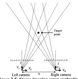
Figure 1-1: Solar panel assembly by cooperative robots... Figure 1-2: Rocky 7 inspecting rock sample... Figure 1-3: Representative physical system... Figure 1-4: Conventional control architecture... Figure 1-5: Physical model based sensor fusion... Figure 2-1: Representation of a general mobile field robot... Figure 2-2: Representation of the simplified mobile robot... Figure 2-3: Flow-diagram of a Kalman Filter... Figure 2-4: Constant parameter arm motion... Figure 2-5: Variable parameter arm motion... Figure 2-6: Mutual information metric for Stiffness Op...,... Figure 2-7: Example of identification converge curves... Figure 2-8: Experimental mobile manipulator... Figure 2-9: Constant parameter arm motion... Figure 2-10: Variable parameter arm motion... Figure 2-11: Inclinometer pitch reading (radians)... Figure 2-12: Example of identification converge curves... Figure 3-1: Cooperative mapping by robots... Figure 3-2: Outline of model building and placement algorithm... Figure 3-3: Flowchart of the initialization of environment mapping algorithm... Figure 3-4: 3-D range measurement fusion with sensor uncertainty... Figure 3-5: Stereo imaging error evaluation...

(8)

Figure 3-6: Sample of merging two Gaussian probability distributions (2-D case).. 55

Figure 3-7: Flowchart for data fusion using known vision system motion... 56

Figure 3-8: Evaluation of expected new information... 58 Figure 3-9: Flowchart for vision system pose selection of environment mapping

alg o rith m ... 6 0 Figure 3-10: Relationship of camera and target frames... 61 Figure 3-11: Flowchart for vision system motion identification using scene

fid u cials... 6 5 Figure 3-12: Unstructured planar environment... 66 Figure 3-13: Results of single vision system modeling an unknown environment... 67 Figure 3-14: Single vision system path... 68 Figure 3-15: Single vision system area mapped (gray=empty space,

black=obstacle, w hite=unknow n) ... 68 Figure 3-16: Results of two vision systems modeling an unknown environment... 69 Figure 3-17: Two cooperating vision systems path... 70 Figure 3-18: Two cooperating vision systems area mapped (gray-empty space,

black=obstacle, w hite=unknow n)... 70 Figure 3-19: Unstructured indoor-type planar environment... 71 Figure 3-20: Results of single vision system modeling an unknown environment... 72 Figure 3-21: Single vision system path... 72 Figure 3-22: Experimental mobile vision system modeling an unstructured

en v ironm en t... 73 Figure 3-23: Identification and tracking of 6 fiducials (o--tracked with previous

(9)

im age, 0--tracked w ith next im age)... 74

Figure 3-24: Accumulated r.m.s. translation error of vision system... 74

Figure 3-25: Number of mapped environment points as a function of scan number 75 Figure 3-26: Environment Environment mapped/modeled-Sequential cam era pose selection... 75

Figure 3-26: Environment Environment mapped/modeled-Maximum information based camera pose selection... 76

Figure 4-1: Cooperative assembly by robots... 78

Figure 4-2: Task directed optimal camera placement... 79

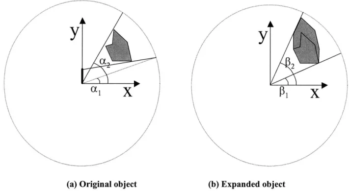
Figure 4-3: Target reduction and occlusion expansion... 82

Figure 4-4: Projection of expanded object... 83

Figure 4-5: Computing the TFVRF (shaded regions)... 83

Figure 4-6: Difference between true and expanded object occluded regions... 84

Figure 4-7: Target angular visibility... 85

Figure 4-8: Optimal camera placement... 87

Figure 4-9: Cooperative assembly concept... 88

Figure 4-10: Simulated planar environment... 89

Figure 4-11: Optimal camera placement with moving object (known CAD model) 90 Figure 4-12: Experim ental test... 92

Figure 4-13: Experimental test-Camera view of target from optimum pose... 93

Figure 5-1: Cooperative insertion task layout... 94

Figure 5-2: Cooperative task target model- representaive problem... 96

(10)

Figure 5-4: Cooperative task target model- relating the coordinate frames of the

cooperatin g rob ots... 97

Figure 5-5: White circular markers to locate object and insertion site... 98

Figure 5-6: Model based sensor fusion from a sensor suite... 99

Figure 5-7: H istogram of im ages... 101

Figure 5-8: Example of image reduction process... 101

Figure 5-9: Circle defined by three points... 102

Figure 5-10: Identification of marker ( centermost hole with 0.25" diameter) ... 104

Figure 5-11: Intermediate steps during task execution (success) ... 105

Figure 5-12: Camera view (stereo pairs) ... 106

Figure 5-13: Optimal camera placement-successful task execution... 107

Figure 5-14: Random camera placement-unsuccessful task execution... 107

Figure A-1: Block diagram of linear feed-forward compensation for dynamic disturbance rejection ... 124

Figure A-2: Representative physical system... 125

Figure A-3: Cooperative robot modeling... 125

Figure A-4: Dynamic tip-over stability... 130

Figure A-5: Environment contact states... 131

Figure A-6: Relation of interacting forces, contact points and measured forces/torqu es... 132

Figure A-7: Error of contact point location w.r.t. sensor noise... 133 Figure A-8: Decentralized cooperative control architecture using surrogate

sen sin g ... 13 3

(11)

Figure A-9: Physically cooperating mobile robots... 134

Figure A-10: Endpoint position and force of master robot and slave robot... 134

Figure A-11: Arm joint and base position of master robot and slave robot... 135

Figure A-12: Arm joint and base forces of master robot and slave robot... 135

Figure B-1: Force/m om ent balance... 136

Figure B-2: Force/moment balance of compliance module... 137

Figure B-3: Representation of the simplified mobile robot... 139

Figure B-4: Force/m om ent balance... 139

Figure B-5: Force/moment balance of compliance module... 140

Figure C-1: LZW com pression flowchart... 146

Figure C-2: Comparison of 2-D image compression methods... 148

Figure D-1: FSRL Experimental cooperative rovers... 149

Figure D-2: Experimental system: 4 DOF manipulator kinematics... 150

Figure D -3: PW M m otor control circuit... 151

Figure D-4: Overview of experimental system hardware... 152

Figure E-1: BR A ID design concept... 157

Figure E-2: ith parallel link stage... 159

Figure E-3: Projection of section ABCD from Figure E-3... 160

Figure E-4: Projection of section EFGH from Figure E-3... 161

Figure E-5: Workspace of 5 stage BRAID element... 163

Figure E-7: SMA power and control bus... 164

Figure E-8: SMA power bus address decoding and latching electronics... 166

(12)

List of Tables

Table 2-1: Simulation parameter identification... 41

Table 2-2: Experimental parameter identification... 45

Table 4-1: Results of changing task difficulty, occlusion density and task execution success... 9 1 Table 5-1: Task execution success for varying task difficulty levels... 105

Table C-1: Comparison of compression methods on 2-D images... 147

Table D-1: Inclinometer calibration data at room temperature... 153

Table D-2: Camera specifications... 154

(13)

Chapter

1 Introduction

1.1. Problem Statement And Motivation

Human exploration and development of the planets and moons of the solar system are stated goals of NASA and the international space science community [Huntsberger-3]. These missions will require robot scouts to lead the way, by exploring, mapping, seeking or extracting minerals and eventually constructing facilities in complex terrains. Multiple cooperating robots will be required to set up surface facilities in challenging rough terrain for in-situ measurements, communications, and to pave the way for human exploration of planetary surfaces (see Figure 1-1). Tasks may include building permanent stations and fuel generation equipment. This will require the handling of relatively large objects, such as deploying of solar panels and sensor arrays, anchoring of deployed structures, movement of rocks, and clearing of terrain. Robots will also assist future space explorers.

Such future robotic mission scenarios suggest that current planetary rover robots, with their limited functionality, such as simple rock sampling (see Figure 1-2), will not be sufficient for such missions [Baumgartner, Huntsberger-2, Parker]. A new generation of planetary worker robots will be essential for future missions [Baumgartner, Huntsberger-1, Huntsberger-2, Huntsberger-3, Schenker]. In addition to the exploration and development of space, such robotic systems could prove vital in earth-based field applications including environment restoration, underground mining, hazardous waste disposal, handling of large weapons, and

(14)

assisting/supporting humans in field tasks [Huntsberger-1, Huntsberger-2, Khatib-2, Osbom, Schenker, Yeo, Walker, Shaffer].

Figure 1-1: Solar panel assembly by Figure 1-2: Rocky 7 inspecting rock sample cooperative robots

Substantial previous research has been devoted to control and planning of cooperative robots and manipulators [Choi, Khatib-1, Khatib-2, Marapane, Parker, Pfeffer, Takanishi, Veloso-1, Veloso-2, Yeo, Donald, Mataric, Gerkey, Alur]. However, these results are largely inapplicable to mobile robots in unstructured field environments. In simple terms, the conventional approach for the control of robotic systems is to use sensory information as input to the control algorithms. System models are then used to determine control commands. The methods developed to date generally rely on assumptions that include: flat and hard terrain; accurate knowledge of the environment; little or no task uncertainty; and sufficient sensing capability. For real field environments, a number of these assumptions are often not valid.

For example, Figure 1-3 shows two physically interacting cooperative robots working in an unstructured field environment. The mobile robotic systems have independently mobile cameras and other onboard sensors, and are working together to assemble a large structure. However, visual sensing is limited due to target occlusions by the object being handled and

Chapter 1 14

(15)

objects in the environment (e.g. rocks, building supplies, drums of materials, debris). There is significant task uncertainty in relative pose between the robots and the target, the grasp points, etc. Due to these limitations and uncertainties, classical robot control and planning techniques break down (see Figure 1-4).

Independently mobile camera

Physical Model of

Sensors _{Robot(s), Task and}

il Environment

Force/Torque Mobile vehicles _Incomplete

Sensor with suspensions _Knowledge

Onboard sensors Control and

ncelrometer,c.) Physical System Planning

Algorithm

Figure 1-3: Representative physical system Figure 1-4: Conventional control architecture The key problem is that it is difficult or impossible to directly measure key information required for the control of interacting cooperative mobile field robots.

1.2. Purpose Of This Thesis

The objective of this research is to develop algorithms to compensate for sensor limitations and enable multiple mobile robots to perform cooperative tasks in unstructured field environments. The key theme is to develop optimal information gathering methods from distributed resources.

The proposed approach in this research is to use physics based models to fuse available sensor information with predictive models that can be used in lieu of missing sensory information. In other words, the physical models of the interacting systems are used as the "sensor fusion engines." Observing these models will provide virtual or surrogate sensing. This virtual sensor information will be used to supplement the incomplete and insufficient direct

(16)

sensor data based on the information obtained from all the members of the robot workers (crew). Thus, experiences (measurements) of each individual robot become part of the collective experience of the group. Such a methodology fuses dynamic models, available sensor data, and prior sensed data from multiple robot team members. This inferred information can be applied to robot control and planning architectures. Figure 1-5(a) outlines this idea. Figure 1-5(b) shows a possible sensor suite of a robot or team of robots, fused using a physics based model, to yield surrogate sensory information.

Sensor I information

Sensor N Direct sensor information

information information

(incomplete)

Multi robot stem

Control and

multi-sensor input Physical P lmoin

with placement system(s) gorithm

optimization a

(a) Control architecture with surrogate sensing

SENSOR SUITE FOR EACH ROBOT

SENSORS MEASURING THE ENVIRONMENT E/M SPECTRUM TACTILE

-2D camera -force/torque sensor AUDITORY ODOR

-lateral photo effect detectors -pressire transsducers -altrasonic seinsois -specrroscopic

-JR proximity sensors -strain gauges -microphones -chemical detection

-NMR -whiskeis/bumpers -etc. -etc.

- adar ltsermal - sesors Physical Task

-etc. -etc e model

based based

opstimizatprionio

SENSORS MEASURING THE ROBOT

PROPRIOCEPTIVE VESTIBULAR -2 rchometer c -inclinometer

-~ eoders -accelerometer i -linear transducers -r aote gyroscopes

- ptary transducers -compass

-etc. k- etc .

(b) Sensor suite example-used in model based fusion Figure 1-5: Physical model based sensor fusion

The approach to this research is divided into three parts "know one's self', "know one's

Chapters 1 16elrmee

(17)

environment" and "know one's task". Fundamentally this reduces to the following. First, field robots must have a good dynamic model of themselves to be used in model-based control algorithms. Second, the robots must have a good geometric environment model in which the task is being performed. Third, the robots must have a good view of the targets critical to performing the task. Algorithms in each successive step use the algorithms developed in the previous steps.

(a) Know ones self: Here, an algorithm is developed to allow a robot to measure its dynamic parameters in the presence of noisy sensor data. These parameters are required to successfully apply model-based control algorithms [Hootsman]. These parameters may be roughly known from design specifications or found off-line by simple laboratory tests. However, for field systems in hostile environments, they may not be well known, or may change when the robot interacts with the environment. For example, temperature fluctuations result in substantial changes in vehicle suspension stiffness and damping. Vehicle fuel consumption, rock sample collection, etc. cause changes in the location of the center of gravity, mass and inertia of the system. Hence, on-line identification of these parameters is critical for the system performance.

(b) Know one's environment: Here, an algorithm is developed to allow multiple cooperating robots to efficiently model/map their environment. For robots working in unstructured environments, it is often not possible to have a-priori models of the environment. The robots will need to build these models using available sensory data. A number of problems can make this non-trivial. These include the uncertainty of the task in the environment, location and orientation uncertainty in the individual robots, and occlusions (due to obstacles, work piece, other robots).

(18)

observe their task effectively. Once the environment model is created, the robots need to position their sensors in a task-directed "optimal" way. That is, for a given task requiring visual guidance, there is an associated target to observe. For example, in assembly tasks, the target may be a single point or region in the environment, a distance between two objects, etc. The algorithm finds optimal view poses of the target for the individual robots as the task is carried out. These view poses provide the required visual guidance for task execution. 1.3. Background And Literature Review

There has been significant research in the area of cooperative robotics over the past decade [Choi, Clark, Khatib-1, Khatib-2, Luo, Marapane, Parker, Pfeffer, Schenker, Takanishi, Veloso-1, Veloso-2, Yeo, Donald, Mataric, Gerkey, Alur]. Relevant research is broken down into four areas: (a) Control and planning of cooperative mobile robots, (b) identification of system dynamic parameters, (c) environment modeling and (d) task modeling.

1.3.1. Control and planning cooperative mobile robots

Aspects of control and planning of cooperative mobile robots have been addressed by a number of researchers, including modeling the environment and task, modeling the physical interactions among robots and between robots and the environment, and assigning individual robot roles [Khatib-1, Marapane, Parker, Donald, Mataric, Gerkey, Alur]. A typical approach to the problem of modeling environment and task knowledge is to assume that both the environment and the task are well-defined or can be obtained with sufficient accuracy [Choi, Khatib-1, Khatib-2, Pfeffer, Donald, Mataric, Gerkey]. Further, many successful approaches have been developed to model dynamic interactions during cooperative manipulation of objects. These include: generating virtual linkages that account for internal forces; augmenting the object to provide a dynamic description at the operational point; dynamic hybrid force/position

Chapter 1 18

(19)

compensation across a passive object; and including passive joints in the closed kinematic manipulator-object-manipulator chain [Choi, Khatib-2, Pfeffer, Yeo].

Some researchers have addressed the problem of tip-over stability due to the dynamic effects in a single mobile manipulator system [Dubowsky, Takanishi]. Researchers have also addressed the problem of role assignment in cooperative systems (hierarchical (master-slave) and equipotent team structures) [Khatib, Marapane, Veloso-1, Veloso-2]. Most work in the area of cooperative robots has focused on small laboratory systems that accomplish simple tasks (such as pushing small objects around a table) while avoiding collisions with other robots [Marapane, Parker]. The planning and control algorithms are primarily heuristic, probabilistic or based on fuzzy logic, do not exploit all the physical capabilities of the system, and testing in field environments has been limited.

1.3.2. Identification of dynamic system parameters

Dynamic system models are often used in robot control architectures, to enhance the system performance. Identification of system parameters is a well-studied problem [Alloum, Atkeson, Bard, Ljung, Nikravesh, Olsen, Serban, Schmidt, Soderstorm]. Various effective algebraic and numerical solution techniques have been developed to solve for unknown parameters using dynamic system models [Bard, Gelb, Nikravesh, Serban]. These include techniques based on pseudo-inverses, Kalman observers, Levenberg-Marquardt methods, and others. However, the accuracy/quality of the identified system parameters is a function of both the system excitation and the measurement noise (sensor noise). A number of researchers have developed metrics to evaluate the quality of identified system parameters [Armstrong, Gautier, Schmidt, Serban, Soderstorm]. Such metrics determine if a given set of parameters is identifiable, which is known as the "identifiability/observability" problem [Serban]. These include tests based on differential

(20)

algebra, where a set of differential polynomials describes the model under consideration [Bard, Ljung]. Other metrics monitor the condition number of an excitation matrix computed from the dynamic model. Examples of such excitation matrices include the Hessian of the model residual vector, the derivative of the system Hamiltonian, and the input correlation matrix [Serban, Gautier, Armstrong].

The metrics of parameter quality can be used to select the excitation imposed on the physical system and have been applied with limited success to industrial robotic systems [Armstrong, Atkeson, Gautier, Mayeda]. However, such approaches can be computationally complex, an important issue for space robots where computational power is very limited. For example, defining excitation trajectories for the identification of an industrial 3 DOF manipulator using an input correlation matrix requires 40 hours of VAX (40MHz) time [Armstrong, Gautier]. Additionally, these methods are unable to indicate which parameter estimates have low confidence values (low quality), since the quality metrics combines the performance into a single parameter. Thus it is not possible to assign higher weight to parameters of greater dynamic significance to system response.

1.3.3. Environment modeling

Environment modeling/mapping by mobile robots falls into the category of Simultaneous Localization and Mapping (SLAM). In such algorithms, the robot is constantly localizing itself as it maps the environment. Several researchers have addressed this problem for structured indoor-type environments [Asada, Burschka, Kruse, Thrun-1, Kuipers, Yamauchi, Castellanos, Leonard, Anousaki, Tomatis, Victorino, Choset]. Sensor movement/placement is usually done sequentially (raster scan type approach) or by following topological graphs [Choset, Victorino, Anousaki, Leonard, Kuipers, Rekleitis, Yamauchi]. Geometric descriptions of the environment

Chapter 1 20

(21)

have been modeled in several ways, including generalized cones, graph models and Voronoi diagrams, occupancy grid models, segment models, vertex models, convex polygon models [Brooks, Choset, Crowley, Kuipers, Miller, Weisbin]. The focus of such work is accurate rather than efficient mapping process. Further, the environment is assumed to be effectively planar (e.g. the robot workspace is the floor of an office or a corridor) and readily traversable (i.e. terrain is flat and obstacles always have a route around them) [Anousaki, Thrun-1, Yamauchi, Choset, Kuipers, Lumelsky].

Localization is achieved by monitoring landmarks and their relative motions with respect to the vision systems. Several localization schemes have been implemented, including topological methods such as generalized voronoi graphs and global topological maps [Choset, Kuipers, Tomatis, Victorino], extended Kalman filters [Anousaki, Leonard, Park], and robust averages [Park]. Additionally, several different sensing methods have been employed, such as camera vision systems [Castellanos, Hager, Park], laser range sensors [Tomatis, Victorino], and ultrasonic sensors [Anousaki, Leonard, Choset]. Although some natural landmark selection methods have been proposed [Hager, Simhon, Yeh], most SLAM architectures rely on identifying landmarks as corners or edges in the environment [Anousaki, Kuipers, Castellanos, Victorino, Choset, Leonard]. This often limits the algorithms to structured indoor-type environments. Others have used human intervention to identify landmarks [Thrun-1].

Some studies have considered cooperative robot mapping of the environment [Jennings, Rekleitis, Thrun-2]. Novel methods of establishing/identifying landmarks and dealing with cyclic environments have been introduced for indoor environments [Jennings, Thrun-2]. In some cases, observing robot team members as references to develop accurate maps is required [Rekleitis].

(22)

1.3.4. Task modeling-visual sensing strategy

Previous work in visual sensing strategies can be divided into two areas [Luo, Tarabanis]. One area is concerned with sensor positioning i.e. placing a sensor to best observe some feature, and selecting a sensing operation that is most useful in object identification and localization. Researchers have used model-based approaches, requiring previously known environments [Burschka, Cowan, Hutchinson, Kececi, Laugier]. Target motions (if any) are assumed to be known [Laugier]. Brute force search methods divide the view volume (into grids, octrees, or constraint sets), and search algorithms for optimum sensor location are applied [Connolly, Cowan, Luo, Kececi, Nelson]. These methods require a priori knowledge of object/target models [Tarabanis, Chu]. Such methods can be effective, but are computationally expensive and impractical for many real field environments, where occlusions and measurement uncertainties are present.

The other direction of research in visual sensing strategies is sensor data fusion i.e. combining complementary data from either different sensors or different sensor poses to get an improved net measurement [Smith, Marapane, Nelson, Tarabanis, Veloso-1]. The main advantages of multi-sensor fusion are the exploitation of data redundancy and complementary information. Common methods for sensor data fusion are primarily heuristic (fuzzy logic) or statistical in nature (Kalman and Bayesian filters) [Betge-Brezetz, Luo, Repo, Clark, Marapane, Nelson, Tarabanis].

For target model building both sensor positions and sensor fusion play key roles. However, current methods do not effectively combine these methods to develop a sensing strategy for robot teams in unstructured environments.

In general, current research has not solved the problem of controlling multiple mobile

Chapter 1 22

(23)

robots performing cooperative tasks in unstructured field environments, where limited sensing capabilities and incomplete physical models of the system(s)/environment dominate the problem. 1.4. Outline Of This Thesis

This thesis is composed of six chapters and five appendices. This chapter serves as an introduction and overview of the work, and summarizes related research.

Chapter 2 addresses the problem of "knowing ones self'. It presents a new information-based performance metric for on-line dynamic parameter identification of a multi-body system. The metric is used in an algorithm to optimally regulate the external excitation required by the dynamic system identification process. This algorithm is applied to identify the vehicle and suspension parameters of a mobile field manipulator. Simulations and experiments show the effectiveness of this algorithm.

Chapter 3 addresses the problem of "knowing ones environment". An algorithm based on iterative sensor planning and sensor redundancy is proposed to enable field robots to efficiently build 3D models of the environment. The algorithm uses measured scene information to find new camera poses based on information content. Simulations and experiments show the effectiveness of this algorithm.

Chapter 4 addresses the problem of "knowing ones task". Here, an algorithm is proposed to enable field robots to efficiently position their cameras with respect to the task/target. The algorithm uses the environment model, task/target model, measured scene information and camera models to find optimum camera poses for vision guided tasks. Simulations and experiments show the effectiveness of this algorithm.

Chapter 5 presents an experimental example of vision-guided cooperative assembly by mobile robots in unstructured field environments. Here, the algorithms developed in Chapters 2,

(24)

3 and 4 are combined.

Chapter 6 summarizes the contributions of this thesis and presents suggestions for future work.

The appendices to this thesis give detailed information on specific topics related to the work presented. Appendix A presents a cooperative mobile robots dynamic model used for model predictive control. Appendix B presents the derivation of the equations of motion of a mobile robot model used in Chapter 2. Appendix C presents a description of loss-less image compression schemes that is used for quantifying information content in a scene. Appendix D describes the Field and Space Robotics Laboratory cooperative rover test-bed, which is used to experimentally validate much of this work. Appendix E presents a concept for a lightweight hyper-redundant binary manipulator that may used for camera/sensor placement tasks.

Chapter 1 24

(25)

Chapter

2 Dynamic Parameter Identification

2.1. Introduction

The first step in compensating for robot model uncertainty is to develop an algorithm that allows field robots to measure their dynamic parameters in the presence of noisy sensor data. These parameters are required to successfully apply model-based control algorithms

In this chapter a new performance metric, called a mutual information-based observability metric, is presented for on-line dynamic parameter identification of a multi-body system. This metric measures the uncertainty of each parameter's estimate. This measure is termed the "parameter observability." The metric is used to formulate a cost function that optimally controls the external system excitation during the identification process. The cost function weighs each parameter estimate according to its uncertainty. Hence, the excitation is controlled so that the identification favors parameters that have the greatest uncertainty at any given time. Parameters may also be given greater importance in the cost function based on its significance to the system's dynamic response. This method is more computationally efficient and yields faster convergence than single parameter methods [Armstrong, Gautier, Schmidt, Serban, Soderstorm].

Here the algorithm is applied to the on-line parameter identification of a mobile field robot system and is shown to be computationally efficient. A field robot may be equipped with a manipulator arm and onboard sensors such as inclinometers, accelerometers, vision systems, and force/torque sensors (see Figure 2-1). An onboard manipulator arm (with bandwidth constraints)

(26)

is moved to generate reaction forces, which excite vehicle base motions. The dynamic parameters include the mass, location of center of gravity, inertia, base compliance and damping.

The method assumes a robotic system composed of rigid elements, and there is no relative motion of the vehicle wheels with respect to the ground during the identification process. The algorithm also assumes that the robot is equipped with an inclinometer, accelerometer and arm base force/torque sensor mounted at the manipulator base. It is assumed that the onboard manipulator dynamic parameters are known, and the bandwidth of the arm actuators is sufficiently high to excite the vehicle dynamics. Finally, the motions of the base compliance are assumed to be small. Multi-DOF Payload Sensor suite 4-Force/Torque sensor suspension

Figure 2-1: Representation of a general mobile field robot

The system is modeled using a Newton-Euler formulation (section 2-2). A Kalman filter is used to solve the dynamic parameters based on the physical model (section 2-3). The mutual information-based observability metric is used to determine the arm excitation trajectory (sections 2-4 and 2-5). Simulation and experimental results show the effectiveness of this algorithm (section 2-6).

2.2. System Dynamic Model

The algorithm to generate arm excitation trajectories for parameter identification requires a

(27)

dynamic model of the system. A number of models of vehicle suspension systems have been proposed [Alloum , Halfmann, Harris, Majj ad, Nelles]. Many of these are quarter or half-vehicle models that consider stiffness and damping coefficients, but neglect vehicle mass and inertial properties. Here, a Newton-Euler formulation is used to model the full spatial dynamics of the system. The system represented in Figure 2-1 is reduced to three components: a rigid arm, a rigid vehicle body and a compliance module (see Figure 2-2). Rotational motions of the rigid arm result in reaction forces/moments felt by the vehicle base and in the suspension module. Motions of the base are measured through the onboard inclinometer, accelerometer and directional compass. Interaction forces/torques between the arm and vehicle base are measured by a base force/torque sensor (origin coincides with frame VI-Figure 2-2).

Vehicle c.m. IV

6 DOF Vehicle

1 suspension

F Vehicle chassis

(does not move)

Figure 2-2: Representation of the simplified mobile robot

Although real vehicles have complex, multi-element suspension systems, only the net base compliance is modeled. This is modeled as a 6 DOF linear stiffness and damping system, located at the vehicle base center-of-gravity (see Appendix A). From the equations derived in Appendix

(28)

A, it can be seen that for small base motions, this simplified model can accurately model the vehicle dynamics. An advantage of the simplified model is that all coefficients can be identified by observing only the vehicle base motions, thus eliminating the need for more exotic sensors placed at each individual suspension. Additionally, a simplified suspension model accounts for all sources of compliance that would be difficult to model and measure individually.

Appendix B presents the dynamic model of the mobile robot presented in Figure 2-2. From Equation B-4, a set of 6 dynamic equations is obtained (forces and moments in 3D):

mi(d(R-'g)-d(i)₁ -bT -dil -k -dr = d(F,

0 Fii 2(2-1)

-Id() 11 - d(6x(I10)) - d(r2 x -b -F) T d6-k -Od = d(N) (

where F12 and N12 are the arm base reaction forces and moments, m2 and 12 are the arm mass and

inertia tensors, a2 and O2 are the arm linear acceleration and angular velocity vectors, Foi and No,

are the suspension reaction forces and moments, mi and I1 are the base mass and inertia tensors, a, and o, are the base linear acceleration and angular velocity vectors, kr and ke are the translational and rotational stiffness coefficients, b, and bo are the translational and rotational damping coefficients. Using the onboard sensors described above, this set of equations present the following unknowns, knowns, and measureable quantities:

unknowns: mi, 1₁, r2, kr , br, k, bo

knowns: m2, 12

measured: dr, di,, di, (III w.r.t. II), dO, d6, d (II w.r.t. I), dF12, dN12

By measuring the motions induced by three rotation modes or the arm (rotation about the x, y and z axes in Frame IV-see Figure 2-2) and applying the six dynamic equations of motion, results in a total of 18 independent equations. Note that the arm rotation motions about the x, y and z axes are done individually, and require rotation of only the arm base joints (Frame IV-see Figure 2-2). The remaining joints are held fixed. This configuration is sufficient to produce the

(29)

dynamic forces required to generate needed vehicle excitations. Additionally, this maintains the generality of the algorithm developed in this chapter, as no specific manipulator kinematics are assumed (other than two base rotational joints).

2.3. Estimating The Dynamic Parameters

To solve for the unknown parameters, Equation 2-1 is first recast into the form A x = F (where A is a known matrix of measured position values, x is the vector of unknowns, and F is a known vector of measured forces/torques). Two common methods to solve equations in the form A x =

F are pseudo-inverse and Kalman filters. Both result in a least-squares solution to the problem. In a pseudo-inverse solution process, a discrete set of measurements combined with the 18 equations are used to formulate the matrix A and the vector F. A solution to A x = F is simply given by: x=(ATA)-'ATF.

A more efficient solution is to use a Kalman filter [Gelb]. A Kalman filter is a multiple-input, multiple-output digital filter that can optimally estimate the states of a system based on noisy measurements. The state estimates are statistically optimal in that they minimize the mean-square estimation error. Here, rather than estimating x based on one large matrix A containing all the position measurements, x is estimated based on a single set of measurements and an associated covariance matrix. With each new measurement set, the estimate is improved and the covariance updated. Since there are numerous articles in the literature describing Kalman filters, only a flow-diagram of the process is presented here (see Figure 2-3) [Bard, Gelb, Nikravesh]. In Figure 2-3, Qk models the uncertainty which corrupts the system model, Rk models the uncertainty associated with the measurement and Ck gives the total uncertainty of the state estimate.

(30)

K P H T H P T + dUpdate estimate F P F T kl klk-I k [k k klk-1l k k/kk +Q Pk/k _[IKk_H _I~k-I_/ X~ state vector : x k1 Fkx + Wk

state noise (w k) _{covariance :}Q _k

measurement vector : zk = Hk xk + vk

measurement noise (vk)covariance : Rk

Figure 2-3: Flow-diagram of a Kalman Filter 2.4. A Metric For Observability

Although the above methods (pseudo-inverse and Kalman filter) produce solutions to the unknown dynamic parameters, a fundamental issue on the observability of unknown parameters is still to be addressed. Essentially, this provides a measure of accuracy of the current solution for the specific dynamic parameter. This is a difficult issue and a-priori tests are not available. 2.4.1. Classical observability metric

Classically, the concept of observability in the control literature is defined from a state model of the dynamic system. The idea is to determine if there are a sufficient number of independent equations relating the system states (from which these states may be inferred). Formally, a system is observable if the initial state can be determined by observing the output for some finite period of time. This metric is briefly outlined here and a discrete formulation is presented.

The linear system model (or state model) for a typical process in the absence of a forcing function is given by:

P,-k=0

Xk+1,k

Ik+llk

(31)

x = FY + Gii7 state model _(2-2) Z = HY + i- observation model

The discrete model is implemented by converting the continuous time model, given by:

Xk+1 = kXk + FkWk state model

(2-3)

Zk = Hk!k + Vk observation model

where

Xk is the (n x 1) system state vector at time tk

Dkis the (n x n) transition matrix which relates xk to Xk+l

Fk is the (n x n) process noise distribution matrix

Wk is an (n x 1) white disturbance sequence with known covariance structure

zk is an (m x 1) measurement at time _tk

Hkis an (m x n) measurement matrix or observation matrix

Vk is an (m x 1) white measurement noise sequence with known covariance

When the F matrix is constant in time and Equation 2-2 is linear, then the transition matrix is a function only of the time step At, and is given by the matrix exponential:

a) - e FAt = I+FAt+ +... (2-4)

2!

It is assumed that process and measurement noise sequences are uncorrelated in time (white) and uncorrelated with each other. In practice, the transition matrix can often be written by inspection. When At is much smaller than the dominant time constants in the system, a two term approximation is often sufficient [Kelly].

Consider the discrete nth order constant coefficient linear system, 1_{ik+1= D}

kyk , for which

there are m noise-free measurements, zk = Hxk(where k=O...m-1), where each H is an (m x n) matrix. The sequence of the first i measurements can be written as:

(32)

zo = Hxo

zi = Hx = Hx ₀

z2 = Hx2 =HQ 2X0 (2-5)

zi_, ₌_{Hxi, H4'-i 0}

This can be written as the augmented set of equations Z = E'x0. If the initial state is to be

determined from this sequence of measurements, then E = HT HITHT (c) H must have

rank n. This definition is limited, in that it does not account for the effects of noisy data. Additionally, the unobservable state cannot be determined. To address both problems, a new mutual information based metric is proposed below.

2.4.2. Mutual information based metric

Consider a set of possible events with known probabilities of occurance of p1, P2, ... , pn. If there

is a measure of the amount of "choice" involved in selecting an event, H(pi, p2, ... , pn), it is

reasonable to require of it the following properties [Shannon]: 1. H should be continuous in the pi.

2. H(qi, q2,..., q,) is a maximum for qk=l/n for k=1... n. This implies that a uniform probability distribution possesses the maximum uncertainty

3. If a choice is broken down into two successive choices, the original H should be the weighted sum of the individual values of H.

It has been shown that the only H satisfying the three assumptions is of the form [Shannon]:

n

H =-K pi log pi (2-6)

i=I

where K is a positive constant. Now consider the case where the signal is perturbed by noise during transmission i.e. the received signal is not necessarily the same as that sent out by the

Chapter 2 32

(33)

transmitter. Two cases may be distinquished. If a particular transmitted signal always produces the same received signal, i.e. the received signal is a definate function of the transmitted signal, then the effect is called distortion. If this function has an inverse-no two transmitted signals produce the same received signal-distortion may be corrected. The case here is when the signal does not always undergo the same change in transmission. In this case the received signal, Y, is a function of the transmitted signal, X, and a second varible, the noise N: Y=f(X,N). The noise is considered to be a chance variable. In general it may be represented by a suitable stochastic process [Shannon]. A finite number of states and a set of probabilities is assumed: ps,(p,j). This is the probability, if the channel is in state a and the symbol i is transmitted, that the symbol

j

will be received and the channel left in state

P. Thus x and

P range over the possible states, i

over the possible transmitted signals and

j

over the possible received signals. In the case where successive symbols are independently perturbed by the noise there is only one state, and the channel is described by the set of transitional probabilities pi(j), the probability of transmitted symbol i being received as

j

[Shannon].

Thus, if a noisy channel is fed by a source, there are two statistical processes at work: the source and the noise. A number of important entropies can be calculated: the entropy of the source, H(x); the entropy of the output of the channel, H(y); the joint entropy of input and output, H(x,y); the conditional entropies H(ylx) and H(xly), the entropy of the output when the input is known and conversely. In the noiseless case H(y)=H(x). These can be measured on a per-second or per-symbol basis. For a discrete channel transmitting a signal, an analogy with a sensor is made. The signal being read is the true value of the parameter being measured. The signal transmitted is the value that the sensor provides to a computer of the measured value (corrupted by noise).

(34)

The above definitions are used to understand the amount of information being transmitted by such a sensor i.e. the measure for observability. Consider the random variables x and y with joint probability distribution p(xi,yj), 1 :4sN, 1 :4 A. The conditional entropy of x given y is defined

as:

N M

H(x I y)= - p(xi, yj)log2 P(xi Iyj) (2-7)

i=1 j=1

H(xly) can be interpreted as the average amount of uncertainty about x (the true value) after y (the measured value-sensor reading) has been revealed. Some important properties of the conditional entropy can be derived [Shannon]:

(i) H(xjy) 41(x) with equality if and only if x and y are independent (ii) H(x,y) = H(y) + H(xly) = H(x) + H(ylx)

The average amount of information about x contained in y can now be defined in terms of the reduction in the uncertainty of x upon disclosure of y. Denoting this information by In(x,y), define:

In(x,y)= H(x) - H(xly) (2-8)

With property (ii), it is easy to show that:

In(y,x) = H(y) - H(ylx) = In(x,y) (2-9)

Thus, the information about x contained in y is equal to the information about y contained in x. For this reason, In(x,y) is called the average mutual information between x and y. From property (i), In(x,y) ;f with equality iff x and y are independent. As a direct consequence of the definition of In(x,y):

NM, _p(xi,yj)

In(x,y)= 1 p(x,y )log2 ' (2-10)

To develop the relationship p(xi,yj), sensor noise is now modeled. A single observation of a

34

(35)

point (X-) is modeled as a Gaussian probability distribution centered at

Y.

A Gaussian to model uncertainty in sensor data is based on two important observations. The use of the mean and the covariance of a probability distribution function is a reasonable form to model sensor data and is a second order linear approximation. This linear approximation corresponds to the use of a Gaussian (having all higher moments of zero). Additionally, based on the central limit theorem, the sum of a large number of independent variables has a Gaussian distribution regardless of their individual distributions [Kelly]. For example, the canonical form of the Gaussian distribution in 3 dimensions depends on the standard deviations of the measurement, ax,y,z, a covariance matrix (C) and the mean measurement (y5) [Ljung, Nikravesh, Smith]:

p(5I = = () exp 1y Y - T C-

(y-

_x)J

(27ry" / 2 - )I

a 2paXaZX

1

(2-11)

where C =pxyoxyxyy 2 pYZ

where the exponent is called the Mahalanobis distance. For uncorrelated measured data p=O. This can be generalized for an n dimensional sensor. H(x) and H(xly) can be explicitly defined in terms of a given sensor:

H(x) = pi log p, (2-12a)

1

where, for example in a special case of a discrete sensor p = - and n = number of sensor

n discrete states.

(36)

n-1 fJp(X-' j7)dx'

-H(x |y) = qilogqi whereqi = a

i=Op( _{' |}

I

_dx'

min

a = min+{max- min> = min+ (i+1)max- min

n n

and max = maximum sensor reading; (2-12b)

min = minimum sensor reading

p(j' ly) is obtained from Equation 2 -11

In(y,x), reflects the information content of the current estimate of the dynamic parameter being estimated. In other words, increasing certainty of a parameter estimate is reflected in the increasing value of In(y,x) associated with that parameter. This metric makes no assumption on the noise statistics (Gaussian, etc.). It is convenient to establish the details using Gaussian noise.

2.5. Formulation Of Exciting Trajectories

Using the observability metric defined in Section 2.4, a method to formulate the appropriate arm-exciting trajectory is now developed. The idea is to use the observability metric to modify the arm motion, thus increasing the information associated with the dynamic parameter estimates.

From Section 2 a set of differential algebraic equations of motion of the form: Ax = F is obtained. For the robot system in the situation considered here, the arm excitation function is sinusoidal, namely f(t)=ao+a.sin(ot) (Equation B-1). The only parameters that can be varied are the amplitude, frequency and offset of the sinusoidal excitation function i.e. amplitude (a), frequency (o) and offset (ao) of motion of the robotic arm.

Based on the associated information (Section 2-4) for the parameter estimate vector, xk, a

cost function is defined as follows:

Chapter 2 36

(37)

1 In In

Vd)=-j1- 1-1 a a

v In- 2 In x (2 -13)

1 I= In _Yr(

2 Inx Inx 2

where i is summed over the number of dynamic parameters to identify. Inx is the current information associated with parameter estimate xi. In"x is the current maximum information (observability) associated with any of the parameter estimates. The control parameters vector d e R3 consists of the amplitude, frequency and offset of the arm excitation function. Note, in this cost function the information associated with with each parameter is weighted such that parameters with a higher uncertainty receive a higher weight. Further, this cost function may be easily amended to include weightings that reflect the relative importance of the individual dynamic parameters.

A numerical minimization routine is applied to this cost function, by changing the excitation function in amplitude, frequency and offset (the current estimates for the unknowns are used here). By assmbling the terms r(d)into a vector R(d), given as:

R(d) = r(d),..., r,. (d)Y (2-14)

the control parameters d must be chosen so that the residual vector R is as small as possible. The quadratic cost function V(d) of Equation 2-13 becomes:

V(d) = -RT(d)R(d) (2-15)

2

The problem of finding d from V(d) is a nonlinear least-squares problem [Nikravesh]. If the vector R(d), is continuous, and if both first and second-order derivatives are available, then the nonlinear least-squares problem can be solved by standard unconstrained optimization methods.

(38)

Otherwise, a method that requires only the first derivatives of R(d) must be used [Serban]. The first derivative of Equation 2-15 with respect to the design parameters, d, is defined as:

n,

G(d)= Vri(d)r(d) -JT(d)R(d) (2-16)

where J(d) E RnAx is the Jacobian matrix of R(d) with respect to the design parameters. The second derivative of Equation 2-15 with respect to the design parameters, d, is defined as:

nm

H(d)= [Vr (d)ri(d)T ₊_V2_{r(d)r (d)]= J}T _(d)J(d)₊_S(d) _(2-17)

i=1

where S(d) e Rx' is part of H(d) that is a function of second derivatives of R(d). Thus the knowledge of J(d) supplies G(d) and the part of H(d) dependent on first-order derivative information, but not on the second order part S(d). Levenberg-Marquardt methods simply omit S(d), and base the step selection (d') on the approximation given by [Serban]:

V(d + d') = V(d) + GT (d)d'+

I

d'JT (d)J(d)d' (2-18)

2 Equation 2-18 leads to the following optimization procedure:

d(k+]) = d(k) + akd'(k) (2-19)

with

d'(k) - G(d(k))

JT(d(k))J(d(k)) _(2-20)

ak = arg min[V(d ()+ adr(k)]

a

d'(k) given by Equation 2-20 represents a descent direction. Thus, using equations 2-19 and 2-20, the amplitude, frequency and offset of the robot arm are refined during the identification process, leading to an optimal excitation trajectory. Note, in physical systems, evaluation of the information metric and optimization of arm motion should be carried out at time intervals larger

(39)

than the sampling time. This permits the physical system to respond to the changes in arm motion.

2.6. Results

2.6.1. Simulation studies

Two tests have been conducted using a 3D simulation of a mobile robot system with a manipulator and suspension compliance. The first uses a constant parameter excitation function

to drive the arm motion. The second uses a varible paramter excitation fuction (based on the formulation presented above) to drive the arm. The paramter identification results are compared. The system was simulated for 10 seconds. The manipulator arm mass is assumed to be 1Kg and

inertias Ix=0.02kg-m2 _Iy=0.001kg-m2 _{Iz=0.02kg-m2 Ix,=0 kg-iM}2 _lyz= _kg-M2 _{Ixy=O kg-m2. In the}

simulation, sensor data is corrupted by adding white noise of up to 10% of the maximum sensed value. Evaluation of the information metric and refining arm motion occur every 0.4 secs, with a sampling time of 0.005 secs.

For the first case, the constant parameter excitation function is given by the form:

f(t)= ao+a.sin((ot) = n/4 + 27/9.sin(7/2 t) (2-21)

This was chosen based on the arm kinematic and dynamic limitations (i.e. to be well within the

manipulator capabilities). Figures 2-4 and 2-5 show the arm excitation functions for the two test

cases. For a sensor with n-bit precision (i.e. 2" possible values), the maximum mutual information associated with the reading is n bits (i.e. no uncertainty, see Equation 2-9). In both test cases, a 10-bit accuracy sensor is assumed i.e. 210 possible values. Figure 2-6 shows the value for the mutual information metric in identifying the stiffness in O, for the two test cases. It is seen that by using the variable parameter excitation function (as opposed to constant parameter excitation function), the amount of information associated with the unknown parameter, Ine, has