Log Classification in the Hardwood Timber Industry: Method and Value Analysis

(1)

UNIVERSITÉ DE MONTRÉAL

LOG CLASSIFICATION IN THE HARDWOOD TIMBER INDUSTRY:

METHOD AND VALUE ANALYSIS

ALVARO GIL

DÉPARTEMENT DE MATHÉMATIQUES ET DE GÉNIE INDUSTRIEL ÉCOLE POLYTECHNIQUE DE MONTRÉAL

MÉMOIRE PRESENTÉ EN VUE DE L’OBTENTION DU DIPLÔME DE MAÎTRISE ÈS SCIENCES APPLIQUÉES

(GÉNIE INDUSTRIEL) AVRIL 2014

(2)

UNIVERSITÉ DE MONTRÉAL

ÉCOLE POLYTECHNIQUE DE MONTRÉAL

Ce mémoire intitulé :

LOG CLASSIFICATION IN THE HARDWOOD TIMBER INDUSTRY: METHOD AND VALUE ANALYSIS

présenté par : GIL Alvaro

en vue de l’obtention du diplôme de : Maîtrise ès sciences appliquées a été dûment accepté par le jury d’examen constitué de :

M. BASSETTO Samuel, Doct., président

M. FRAYRET Jean-Marc, Ph.D., membre et directeur de recherche M. AGARD Bruno, Doct., membre

(3)

DEDICATION

(4)

ACKNOWLEDGEMENTS

First of all, I’d like to thank to my family, Vanessa and Christopher for helping me during my studies, and being always a support during my long days and nights.

My infinite gratitude is also to my research advisor, Mr. Jean-Marc Frayret, who not only believed in me since the beginning, but also welcomed me in his research team, and encouraged me to follow my research. His experience and great knowledge has given him a wide vision to find the right track every time I was clueless. After the long sessions we spend finding solutions to these and many other dilemmas, I realized that more than a good teacher, he is a great human being. I am proud of have working with him.

All my acknowledgements goes also to Francis Fournier and Jean McDonald of FP Innovations for guiding this research and for providing us the technical information necessary to understand and solve the puzzle we had three years ago when this journey begin.

Finally, I’d like to thank the VCO NSERC network for the financial support and for all the research and networking activities that I had the opportunity to be part of, which gave me the chance to have a better vision of the forest products industry and its challenges.

(5)

RÉSUMÉ

Les industries avec différentes entrées, telles que : l'industrie des produits forestiers (FPI), l'industrie minière ou l'industrie du recyclage, doivent faire face à l'incertitude de matière primaire, ce qui affecte leur capacité à prévoir le rendement de sortie. Pour régler ce problème, les industries peuvent réduire l'incertitude à la source, ou de planifier les opérations en tenant compte de l'incertitude. Dans le FPI, la première approche est généralement utilisée. Par exemple, l'industrie du bois d'œuvre a implémenté des technologies de transformation sophistiquées pour adapter le processus du sciage aux caractéristiques des billes en utilisant la technologie de numérisation pour obtenir des informations précises sur l'état des travaux en cours de fabrication. Une autre approche pour réduire l'incertitude est la classification de matière primaire. Certaines caractéristiques spécifiques peuvent être mesurées à l'entrée pour classer la matière primaire et en conséquence, augmenter la certitude des attentes de production dans chaque classe. Toutefois, si le processus implique les journaux, les minerais des mines ou des papiers recyclés, la classification de matière primaire a une valeur et un coût selon le degré de détail effectué. Cette recherche propose d'abord une méthode basée sur l'analyse des arbres de classification pour classer les billes de feuillus. Ensuite, en utilisant la simulation à base d'agents, nous analysons la valeur des différentes stratégies de classification, de la plus détaillée, à aucune classification. Les résultats montrent dans le cadre de l'industrie du bois de feuillus que l'avantage de classification détaillée est compensé par son coût, tandis qu'une classification relativement simple permet d'améliorer considérablement le rendement de la production.

(6)

ABSTRACT

Industries with variable inputs, such as the forest product industry (FPI), the mining industry or the recycling industry, must cope with material uncertainty, which affects their ability to predict output yields. To deal with this, one can either reduce uncertainty at the source, or plan operations taking uncertainty into account. In the FPI, the first approach is generally used. For instance, the softwood lumber industry has adopted sophisticated transformation technologies that adapt sawing patterns to the log characteristic using scanners technology to acquire accurate information about work-in-process status. Another approach to reduce uncertainty is input material classification. Specific characteristics can be measured to classify input material and therefore reduce uncertainty within each class. However, whether the process involves logs, mining ores or recycled papers, material classification has a value and a cost according to how detailed it is performed. This research first proposes a method based on classification tree analysis to classify hardwood logs. Next, using agent-based simulation, it analyses the value of different classification strategies, from detailed, to no classification at all. Results show in the context of the hardwood lumber industry that the benefit of detailed classification is offset by its cost, while a relatively simple classification dramatically improves output yield.

Keywords: hardwood timber industry; material classification; classification tree analysis;

(7)

LIST OF TABLES

Table 3.1: General procurement information per transformation application ... 10

Table 3.2: Total observations (# of logs) per threshold and second transformation application ... 11

Table 3.3: Average procurement cost per threshold and second transformation application ... 12

Table 3.4: Prediction accuracy per threshold and transformation application ... 13

Table 3.5: Accuracy and average procurement cost of chosen thresholds per application ... 15

Table 3.6: Classification accuracy for each branching level and application at the selected thresholds ... 15

Table 3.7: General class characteristics for each application ... 16

Table 4.1: Correlation matrix of logs yield in each secondary application ... 24

Table 4.2: Aggregation strategies ... 25

Table 4.3: Aggregation strategies applied to the layout zones in the log-yard ... 27

Table 5.1: Total first transformation yield (fbm) per initial stock and strategy ... 29

Table 5.2: Total first transformation yield (fbm) per different product types in the production campaign ... 30

Table 5.3: Average anticipated production yield (fbm) for every strategy and inventory level .... 31

Table 5.4: Average anticipated production yield (fbm) for different product types in the production campaign ... 32

Table 5.5: Average procurement cost for every strategy and inventory level ... 33

Table 5.6: Total procurement cost for different product types in the production campaign ... 33

Table 5.7: Average ratio between total procurement cost and anticipated yield for every strategy and inventory level ($/fbm) ... 34

Table 5.8: Ratio between anticipated yield and total procurement cost for different product types in the production campaign ... 35

(10)

Table 5.10: Loader Utilization for different product types in the production campaign ... 37 Table 5.11: Average number of visits to alternative piles for different initial inventory levels .... 39 Table 5.12: Average number of visits to alternative piles for different product types in the

production campaign ... 39 Table 5.13: Average stock level in the pre-defined zones of the sawmill with an initial inventory

of 0. ... 40 Table 5.14: Average stock level in the pre-defined zones of the sawmill with an initial inventory

of 12,000. ... 40 Table 5.15: Average stock level in the pre-defined zones of the sawmill with an initial inventory

(11)

LIST OF FIGURES

Figure 3.1: Logs statistical distributions of diameter, % of heartwood, sawing time and cost ... 9

Figure 3.2: Classification tree accuracy vs. Average procurement cost per application ... 14

Figure 4.1: Process description ... 18

Figure 4.2: Basic sawmill process model ... 19

Figure 4.3: Layout of the computer simulation model ... 21

Figure 4.4: Production plan possible configurations ... 23

Figure 4.5: Layout arrangement strategies ... 26

Figure 5.1: Total first transformation yield (fbm) per initial stock and strategy ... 29

Figure 5.2: Total first transformation yield (fbm) for different product types in the production campaign ... 30

Figure 5.3: Average anticipated production yield (fbm) for every strategy and inventory level ... 31

Figure 5.4: Average anticipated production yield (fbm) for different product types in the production campaign ... 32

Figure 5.5: Ratio between anticipated yield and total procurement cost for different initial inventory levels ... 34

Figure 5.6: Ratio between anticipated yield and total procurement cost for different product types in the production campaign ... 35

Figure 5.7: Loader utilization for different initial inventory levels ... 36

Figure 5.8: Anticipated production yield (fbm) Vs. Loader utilization ... 37

(12)

LIST OF SYMBOLS AND ABBREVIATIONS

fbm Board-foot: Board foot is the unit of measure for rough lumber (before drying and planing with no adjustments) or planed/surfaced lumber. In French, this unit is represented as PMP (pied mesure de planche). If the measured quantity is in thousands, is common to use mfbm (thousand board-feet).

1fbm = 1ft x 1ft x 1in

(13)

LIST OF APPENDICES

APPENDIX A – CLASSIFICATION EQUATIONS AND DIAGRAMS PER

TRANSFORMATION APPLICATION ... 48 APPENDIX B – JOINT CLASSIFICATION GRID PER TRANSFORMATION APPLICATION ... 51 APPENDIX C – QUALITY A AND B CLASSIFICATION TABLES USED AT THE RECEIVING AREA TO VALUE PRODUCTS ... 52 APPENDIX D – TABLES WITH DETAILED RESULTS OF THE EXPERIMENTS ... 53

(14)

CHAPITRE 1

INTRODUCTION

1.1 Problem statement

A common issue faced by many industries, such as the forest product industry (FPI), the mining industry or the recycling industry, concerns the need to make decision with unreliable or incomplete information. This uncertainty concerns many aspects of decision-making, including demand, input material attributes, cost, prices, quality, and transformation yield. On the one hand, studies have shown that more detailed information can lead to better supply chain performance (D’Amours et al (1999)). On the other, flexibility and agility in manufacturing are instrumental to dealing with input variability (Kouiss et al (1997), Frayret et al (2007)). However, in order to become agile, it is necessary to develop advanced processes and technologies to detect and adapt to changes and variability.

This research proposes an approach to deal with input material variability in the context of the Quebec hardwood timber industry. In this industry, logs have unique and variable attributes. For sawmill managers, unless logs are systematically scanned and somehow tagged when there are delivered, this variability leads to information incompleteness, which in turn, leads to information uncertainty with respect to decision-making. Consequently, it is difficult to predict both the transformation output yield (i.e., sawn timber volume) and mix (i.e., sawn timber attributes and quality).

Traditionally, sawmills managers organize operations and procurement in order to increase total yield, using dimensions and quality parameters based on the NHLA standards (i.e., National Hardwood Lumber Association). Sawmills also produce specific timber dimension and quality according to the specific needs of their customers. Next, timber is transformed into specific secondary products such as floors, cabinets, and palettes. This general transformation strategy assumes that most NHLA standard products provide adequate secondary transformation (i.e., component manufacturing) yields, instead of adapting operations to meet actual demand requirements. This results in inadequate inventory levels of products that do not meet demand expectations, and consequently, a loss of opportunity and profits due to inventory cost and discount sales. This is mainly the consequence of three causes. First, the use of NHLA standards makes hardwood timber a commodity product. Therefore, the industry focuses its continuous

(15)

improvement efforts on yield maximization, in order to increase production volumes. Second, the use of NHLA standards also leads the industry to ignore the specific needs of secondary transformations. In other words, first transformation is not managed in order to optimize demand satisfaction but to minimize timber procurement cost and maximize the resource utilization, leading to the current situation where sawmills are fully used but incapable of optimizing input logs to control output mix. This is emphasized because logs have very different attributes with respect to their physical dimension and quality, which makes it even more difficult to accurately predict the output of every single log.

1.2 Research objectives

The current research was done with real information of a sawmill in Quebec provided by the industrial partner FP Innovations, with a transformation process consisting of four steps (i.e. receiving, classification, storing and sawing). Once the logs are sawed and transformed into small pieces timbers, they are temporary stored and sold to small enterprises where the timbers are transformed according to a final application (i.e. floor, wardrobe, cabinet, molding, etc.). These applications, known as secondary transformation sector, are the ones the final customer usually receives. The volume of timber produced in the first transformation is known as primary yield. Next, the processing of this sawn timber according to a secondary application produces a new volume of final product, known as secondary yield. As it was previously explained, log sorting and transformation is done by using standard quality rules rather than demand requirements, whereas the secondary transformation is focused on the final client’s expectations.

In order to improve sawmill operations control, sawmills have to measure some logs attributes at the receiving area, and use this information to classify logs, and link the production campaigns to the secondary transformation demand. Therefore, the objectives of the research are:

 To propose a novel log classification approach based on secondary transformation needs when only the information of the logs and production campaigns are known;

 To assess the logistic performance of different methodologies of log classification by considering aggregation levels, and therefore, to measure the value of log attributes information.

(16)

1.3 General methodological approach

In order to achieve the two objectives mentioned previously, the general methodology applied in the current research, and described in detail in Chapter 3, consist in two main steps:

1. Since the information of timber attributes is available, we used a statistical method referred to as classification tree analysis, or decision trees, to create classification rules to sort logs according to their ability to produce efficient secondary transformation yield. The classification trees are then merged to create a single classification grid that can be used in the reception area of sawmills to classify logs according to their ability to produce pieces of timber required for specific second transformation needs. In a further stage, the classification trees are re-evaluated to merge some secondary applications in order to reduce the number of groups. The different configurations are known as aggregation strategies.

2. Every aggregation strategy requires a different storage area configuration, and thus, different paths and distances are followed, which means different levels of utilization of the loaders, which transport the logs. Therefore, the second phase of this study is to build a hybrid discrete event and agent-based simulation model to compare the different approaches and find the real benefits of the proposed approach.

The document is divided as follows: Chapter 2 presents a literature review, covering the different approaches used to deal with sawmills optimization and strategies to deal with input variability. In Chapter 3, the detailed methodology used for this research is explained. Chapter 4 presents the simulation and experimentation phase. Chapter 5 presents the results analysis and finally, Chapter 6 presents the study conclusions and further recommendations.

(17)

CHAPITRE 2

LITERATURE REVIEW

The forest product industry (i.e., FPI) has been extensively studied in the scientific community. Especially, the operation research and industrial engineering community has proposed many approaches to maximize output yields and lower cost in many different contexts. Rönnqvist (2003) proposes a complete review of optimization problems in forestry, as well as the most common techniques for solving them. Along the same line, Gunn (2009) proposes a review of mathematical optimization methods for forest management. These two contributions illustrate both the extent of OR applications in forestry, the efficiency of these methods and, indirectly, the potential value of quality information in decision-making.

With a focus on sawmill operations optimization, Maturana, Pizani, and Vera (2010) and Alvarez and Vera (2011) highlight the need for reliable information in the context of robust optimization and heuristic techniques applications. The need to deal with information uncertainty has also been addressed in other contexts of forestry. For instance Beaudoin, LeBel, and Frayret (2007) propose a mixed integer programming approach to support the annual harvest planning process, which uses a Monte Carlo analysis (see below) and a simple rule-based simulation in order to address information uncertainty. Along the same line, Zanjani, Nourelfath, and Ait-Kadi (2009) proposed a multi-stage stochastic programming model for sawmill production planning with input materials and demand information uncertainty. The same authors developed a similar approach, which uses robust optimization for sawmill production planning with random yield (Zanjani, Ait-Kadi, and Nourelfath (2010)). All these technics were proven to be efficient approaches to deal with information variability issues. However, they do not consider the impact of input material information uncertainty on secondary transformation yields, which is addressed in this paper.

Another effective tool for dealing with uncertainty is simulation. In general, computer simulations can be used to better understand the impacts of specific decisions, policies, or systems configurations through the use of computer simulation of real systems. Computer simulations can also be used in educational settings in order to develop specific skills, in which students control part of the computer simulation variables through user interfaces. Beside spreadsheet simulation, there are four main simulation technics, including Monte Carlo simulation, Discrete-Event Simulation, System Dynamics and Agent-Based Simulation.

(18)

Monte Carlo Simulation uses, repeatedly, random sets of numbers from known probability distribution of different sources of uncertainty in order to compute the results of a mathematical model or algorithm (i.e., the system's model), from which we can infer the general behavior or performance of that system. It is used in practice when the behavior of the system cannot be easily calculated analytically. Discrete-Event Simulation aims to create simulation models of queuing-type systems, in which time moves forward either by equal time increments or from one event to the next. Events and flows between system components occur according to known probability distributions specifying processing and transit times and priority rules. Similarly, System Dynamics aims to model complex systems in order to analyze their general behavior. However, System Dynamics uses a top-down modeling approach based on stocks, flows, feedback loops and time delays, in order to simulate the complex interactions between the components of a system. In other words, System Dynamics aims to capture the ripple effect of changes to these components throughout the entire system, in order to model and study the resulting non-linear behavior of the system. System Dynamics only models the mutual dependencies between these components. It does not model the elementary interactions between the individual elements of the system, which is what Agent-Based Simulation aims to model and simulate. Agent-Based Simulation is an emerging simulation tool (Macal & North, 2006), which takes a bottom-up approach to model the individual behaviors and interactions of a system's elements, referred to as agents. Therefore, instead of modeling the relationships between the components a system, Agent-Based Simulation captures how the individual elements of a system behave with respect to their own local environment and state, and how they interact, communicate, make collective decisions, or influence each other. The Agent-Based Simulation modeling paradigm uses theoretical models to capture individual behaviors.

In the timber production context, Reeb (2003) and Grigolato, Bietresato, Asson, and Cavalli (2011) use Discrete-Event Simulation in order to develop production scenarios and forecast production outcomes based on attributes such as length and logs diameter. More recently, in the context of a log yard management, Beaudoin et al. (2013) achieve to reduce the average truck cycle time and the total distance per loader, by changing the allocation strategy, using Discrete-Event Simulation to test several configurations.

Concerning Agent-Based Simulation, Frayret (2011) presents an introduction of agent-based technology applications in the forestry sector. In the specific domain of forest product supply

(19)

chain, several contributions have been proposed (J. M. Frayret et al. (2007), Forget et al, (2008), Yanez et al (2009), Elghoneimy and Gruver (2011)). In these applications, software agents are usually developed to simulate production planning and scheduling decisions and how they are coordinated across the supply chain in response to changing exogenous parameters. These applications are generally used to evaluate production planning methodologies or supply chain coordination technics. Again, these simulation applications are mainly concerned, so far, by forest operations and the first transformation (i.e., sawing, drying, planing). Secondary transformation operations are only modeled as randomly generated purchase orders.

Another important issue dealing with material variability is automated inspection technology. By providing detailed information about input material (i.e., trees, logs, work-in-process timber), these technologies enable the adaption of transformation operations to individual log and WIP attributes. For instance, in the softwood timber industry, scanners are used at different points in the transformation process in order to maximize productions yield. However, for various reasons, this technology is not used in the hardwood first transformation, although advanced applications exist in the furniture industry.

Finally, a practical alternative approach to deal with material variability is material classification. Material classification aims to create classes of material, which attributes are similar, so the transformation of material (e.g., logs) within a class has similar output. More specifically, the characteristics of the finish products made with logs of the same class are similar. Statistical analysis techniques are used to create such classes. For instance, Petutschnigg and Katz (2005) developed a non-linear model that can predict both timber performance according to log diameter and length, and the type of timber, based on historical observations. A similar procedure was used in Zhang & Liu (2006) by applying parametric and non-parametric regression methods to predict lumber volume recovery for black spruce. This technic lead to good results in small and medium sized trees. Finally, Tong and Zhang (2006) used detailed information from scanned logs in order to compute the production yields of a plant using a dedicated software simulation tool called Optitek. Optitek is a simulation tool that aims to predict yields based on log attributes and machine characteristics. This method, similar in part to the approach used in this paper, requires the scanning of a representative sample of logs.

(20)

CHAPITRE 3

LOG CLASSIFICATION METHODOLOGY

This chapter details the methodology used to carry out this research project. First, we introduce the current process and activities found in hardwood sawmills. Next, we present the information available concerning the log sample we used to propose log classes based on their ability to produce high secondary transformation yields.

3.1 General sawmill processes

Usually, when logs are delivered to the sawmill, they are laid down in the receiving area and measured in order to assess their volume and quality according to the NHLA tables, for the sole purpose of paying the supplier. Then, they are transported into different piles according to their species at the log-yard. This simple classification rule only allows production managers to select the logs to transform according to the most general attribute of customer demand (i.e., the species). Specific details about customers' applications are disregarded.

Once the sawing process is started, a loader takes logs from a selected pile in the log-yard and puts them on the feeder of the sawing line, which contains about 60 minutes of workload. Next, they are transformed into several pieces of timber. Such a production campaign aims to transform a specific species, and not to produce specific timber of a second transformation application. The output timber is then planed, sorted, and dried before been sent to a second transformation process, which is usually carried out by other companies.

In this general process, demand information is only used during the timber sorting process, in order to have different piles of timber for different secondary applications. This implies that such production campaigns (also referred to as production plans in the remaining of this work) are planned based on the general attributes of demand (i.e., species), and not on the detailed applications of demand (e.g., furniture, panel, molding).

This current approach has two consequences. The first is the disconnection between production and demand, and the second, the inability of hardwood sawmills to control production output, which leads to missed opportunities.

(21)

3.2 Available information

In order to develop log classes, we used actual data from a typical sample of logs. Data collection was carried out by FPInnovations. To do so, they analyzed the input logs and output products of a sawmill. The sample of logs analyzed included 240 logs of yellow birch, of a total population of 1900 logs transformed in a full work day of an average hardwood sawmill in Quebec (Canada) with two production lines. For each log, the following attributes were known:

 The position of the log in the tree (U or B);

 The log diameter measured under the bark at the small end;

 The number of clear faces;

 The percentage of heart wood, which means the ratio between the diameter of the heart measured at the small end and the log diameter at the beginning of the log;

 The deduction percentage of different defects in the log, such as curvature and decay;

 The log quality based on the Québec Minister of Natural Resources standard (which is used to value logs);

 The sawing time;

 The cost.

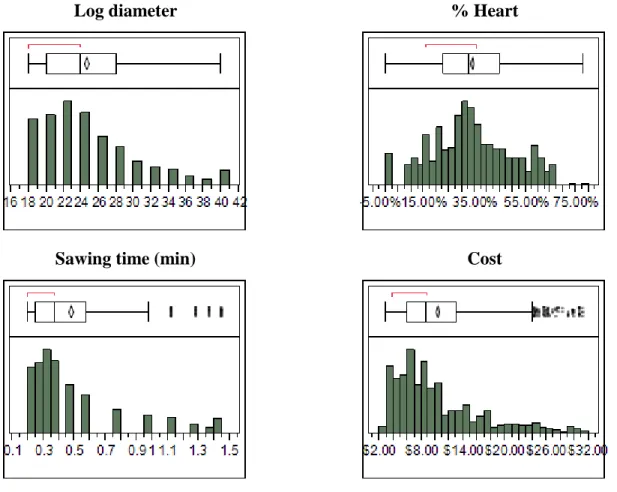
The statistical distributions of the main attributes of these logs are presented in Figure 3.1.

These logs where actually cut into 2150 pieces of timbers, which were then analyzed with BorealScan (Caron, 2005). BorealScan is an industrial scanner developed by the Centre de

recherche industrielle du Québec, which aims to optimize the use of hardwood timber for

appearance wood applications. BorealScan is designed to scan the dimension and appearance of timber and anticipate its expected yield per volume for each type of secondary transformation application (i.e., foot-board produced per cubic meter of log, in fbm/m3, McDonald and Drouin (2010); Drouin, Beauregard, and Duchesne (2010)). These secondary transformation applications are hardwood floor, wardrobe, staircase, paneling, cabinet, moulding and palette.

(22)

Log diameter % Heart

Sawing time (min) Cost

Figure 3.1: Logs statistical distributions of diameter, % of heartwood, sawing time and cost Next, using this yield for each log and each application, and the cost of each log, we computed , the unit cost of timber per 1.000 fbm of secondary transformation component for log l and application a, expressed in $/Mfbm as follows:

unit cost of timber for log l and application a; (1)

with

L set of all logs;

set of useful logs;

nu number of useful logs

A set of secondary transformation applications; log l;

application a; cost of log l;

(23)

In other words, for each specific log, this unit cost represents the procurement cost to produce 1.000 fbm of components of a given secondary application, if all logs had identical attributes. Because not all logs can produce pieces of timber useful for all applications, the term useful log refers here to logs from which we obtained pieces of timber that are useful (i.e., subset ) for a given secondary application (i.e., with a yield greater than zero). Next, we computed , the average procurement cost of logs for all application as follows:

∑

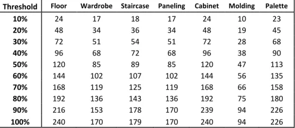
(2) The number of logs with available information and the average procurement cost per application are presented in table Table 3.1.

Table 3.1: General procurement information per transformation application

Floor Wardrobe Staircase Paneling Cabinet Molding Palette # of useful logs

(nu)

240 170 179 170 240 94 226

APC ($/Mpmp) $2,326 $3,498 $2,699 $3,664 $1,271 $6,964 $1,964

The next step is to identify the proper set of attributes to classify the logs according to the target application. To do this, we use classification trees.

3.3 Classification trees

A classification tree is a nonlinear methodology, which uses decision rules to predicting the membership of a case to one of multiples categories based on a set of attributes called the predictor variables. In this data mining technique, the tree is constructed by partitioning the data into a tree-like structure with branches and nodes. At every node, a simple decision rule is defined by creating a linear relation between the independent variable and the binary membership predictor, which becomes the dependent variable.

The selection of the predictor variable at a given node is done using information theory, by measuring the Shannon entropy of every possibilities and selecting the one with the highest information gain (i.e., lowest entropy). The number of branches depends on the type of variable (i.e., quantitative or categorical) and the algorithm used. One of the most effective and popular

(24)

algorithms is the Classification And Regression Tree CART (Breiman, Friedman, Stone, & Olshen, 1984). The partition is repeated until a pre-defined level (i.e. a fixed number of branches) or until a node is reached for which no split improves the information gain. The final nodes are known as terminals, and the resulting equations are used as classification rules.

In the current dataset (240 measured logs), the predictor variables are the logs’ attributes and the dependent variables are the membership binary variables to each second transformation application. In order to apply this method, a classification tree must be built for each application. Since there is insufficient information for all the logs (i.e, not all logs have non-zero yield for all applications as seen in Table 3.2), the first step is to choose how many of the observations (i.e., logs) are relevant for each category (i.e., application). In order to do this, we divided the range of unit cost of timber per application of all logs (i.e., ) into percentiles. This resulted in a matrix of binary values indicating whether or not the log belongs to the percentile.

Table 3.2: Total observations (# of logs) per threshold and second transformation application

Threshold Floor Wardrobe Staircase Paneling Cabinet Molding Palette

10% 24 17 18 17 24 10 23 20% 48 34 36 34 48 19 45 30% 72 51 54 51 72 28 68 40% 96 68 72 68 96 38 90 50% 120 85 89 85 120 47 113 60% 144 102 107 102 144 56 135 70% 168 119 125 119 168 66 158 80% 192 136 143 136 192 75 180 90% 216 153 178 170 239 94 226 100% 240 170 179 170 240 94 226

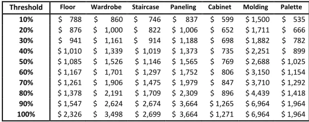
Since the cost Cl and yield for each application of all logs is known, as well as the number of

logs in each percentile (see Table 3.2), we calculated the average procurement cost of each decision tree, with being the set of logs in percentile p and application a (see Table 3.3).

(25)

Table 3.3: Average procurement cost per threshold and second transformation application

Threshold Floor Wardrobe Staircase Paneling Cabinet Molding Palette

10% $ 788 $ 860 $ 746 $ 837 $ 599 $ 1,500 $ 535 20% $ 876 $ 1,000 $ 822 $ 1,006 $ 652 $ 1,711 $ 666 30% $ 941 $ 1,161 $ 914 $ 1,188 $ 698 $ 1,882 $ 782 40% $ 1,010 $ 1,339 $ 1,019 $ 1,373 $ 735 $ 2,251 $ 899 50% $ 1,085 $ 1,526 $ 1,146 $ 1,565 $ 769 $ 2,688 $ 1,025 60% $ 1,167 $ 1,701 $ 1,297 $ 1,752 $ 806 $ 3,150 $ 1,154 70% $ 1,261 $ 1,906 $ 1,475 $ 1,979 $ 847 $ 3,710 $ 1,292 80% $ 1,378 $ 2,191 $ 1,709 $ 2,309 $ 896 $ 4,439 $ 1,418 90% $ 1,547 $ 2,624 $ 2,674 $ 3,664 $ 1,265 $ 6,964 $ 1,964 100% $ 2,326 $ 3,498 $ 2,699 $ 3,664 $ 1,271 $ 6,964 $ 1,964

Next, for all percentiles p and applications a, a decision tree DTpa was built considering only the

attributes of the logs in the selected percentile (i.e., , with being the subset of logs of a

percentile p for application a). The resulting equations at the terminal nodes were used to predict the membership of all logs in the database to each application. The membership of log l to application a and percentile p is noted (i.e., =1 if , 0 otherwise), while the prediction of is noted ̂. In order to measure the accuracy of the prediction, we introduced the binary variable and the prediction accuracy of the decision tree DTpa for

percentile p and application a, as follows:

{ ̂ (3)

∑ _|

| (4)

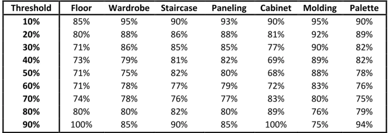
This indicator allows us to evaluate the overall prediction accuracy for each decision tree DTpa,

and its associated threshold (i.e., the value of p), and each application. The of all the computed trees (i.e., for all applications and thresholds) is presented in Table 3.4, showing the high prediction efficiency of the methodology at every level.

(26)

Table 3.4: Prediction accuracy per threshold and transformation application

Threshold Floor Wardrobe Staircase Paneling Cabinet Molding Palette 10% 85% 95% 90% 93% 90% 95% 90% 20% 80% 88% 86% 88% 81% 92% 89% 30% 71% 86% 85% 85% 77% 90% 82% 40% 73% 79% 81% 82% 69% 89% 82% 50% 71% 75% 82% 80% 68% 88% 78% 60% 71% 78% 77% 79% 72% 83% 76% 70% 74% 78% 76% 77% 83% 80% 75% 80% 80% 80% 82% 80% 89% 76% 79% 90% 100% 85% 90% 85% 100% 75% 94%

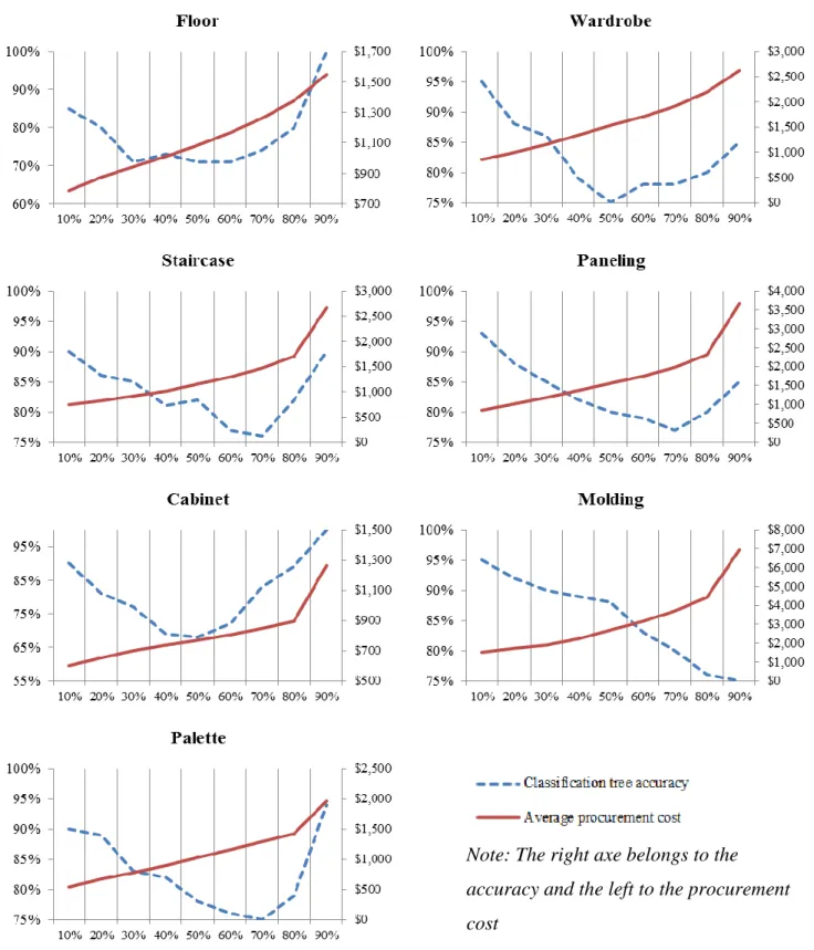
The goal of this step is to find accurate classification rules that simultaneously optimize secondary transformation yield and procurement cost. However, as presented in Table 3.4, the highest values of prediction accuracy are usually related to the largest samples threshold p, which has also a higher procurement cost (see Table 3.3). Therefore, the challenge is to find the right threshold per application, with low procurement cost and high accuracy. Figure 3.2 presents the classification accuracy versus the average procurement cost.

In order to avoid small log samples, which can lead the procedure to exclude several relevant logs, we consider only thresholds higher than 20%. In order to select the most appropriate classification tree for each application, we choose the highest classification accuracy beyond 20% with the lower average procurement cost. Table 3.5 presents the chosen thresholds and the main indicators.

Since the number of independent variables is relatively big, the number of branches found by the classification tree algorithm can also be large. Because the resulting classification rules must be implemented manually in the reception area of the sawmill, the number of branch was first limited to 5 therefore the complexity is relatively low. However, in order to improve the result, we also analyze a wider range of branches during the selection of the threshold for each application. The Table 3.6 presents the classification accuracy for each number of branches (from 4 to 10). The results shows that in most applications, 5 branches leads to good result, although in some cases, fewer branched is enough (i.e. the wardrobe or the paneling application). For other applications, a higher number of branches is necessary, such as a 6-branch tree is needed for the

(27)

floor and staircase applications. The final classification trees are presented in the Error!

eference source not found..

Note: The right axe belongs to the accuracy and the left to the procurement cost

(28)

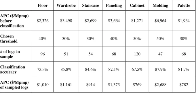
Table 3.5: Accuracy and average procurement cost of chosen thresholds per application

Floor Wardrobe Staircase Paneling Cabinet Molding Palette APC ($/Mpmp) before classification $2,326 $3,498 $2,699 $3,664 $1,271 $6,964 $1,964 Chosen threshold 40% 30% 30% 40% 50% 50% 30% # of logs in sample 96 51 54 68 120 47 68 Classification accuracy 73.3% 85.8% 84.6% 82.1% 67.5% 87.9% 81.7% APC ($/Mpmp) of sampled logs $1,010 $1,161 $914 $1,373 $769 $2,688 $782

Table 3.6: Classification accuracy for each branching level and application at the selected thresholds

Branches Floor Wardrobe Staircase Paneling Cabinet Molding Palette

4 70.8% 85.8% 81.7% 82.1% 64.2% 86.3% 78.3% 5 73.3% 85.8% 84.6% 82.1% 67.5% 87.9% 81.7% 6 75.4% 85.8% 87.5% 82.5% 67.5% 87.9% 83.3% 7 75.4% 85.8% 87.5% 82.5% 68.8% 87.9% 83.3% 8 75.4% 86.7% 87.9% 82.5% 68.8% 87.9% 83.3% 9 75.4% 86.7% 87.9% 82.5% 71.7% 87.9% 83.3% 10 75.8% 87.1% 87.9% 82.5% 72.1% 87.9% 84.2%

Once a classification tree has been found for each application, we calculated the procurement cost per application based on the logs resulting for the use of these classification trees. In other words, since the accuracy of these trees is lower than 100%, the logs predicted to be useful for an application is different from the log sample used to build the trees. Therefore, a different average

(29)

procurement cost is to be expected. Table 3.7 presents the final sample size and average cost per application once the classification trees are applied.

Table 3.7: General class characteristics for each application

Floor Wardrobe Staircase Paneling Cabinet Molding Palette APC ($/Mpmp) before classification $2,326 $3,498 $2,699 $3,664 $1,271 $6,964 $1,964 Chosen threshold 40% 30% 30% 40% 50% 50% 30% # of branches 6 4 6 4 5 5 5 # of logs after classification 109 53 44 53 72 26 78 Classification accuracy after classification 75.4% 85.8% 87.5% 82.1% 67.5% 87.9% 81.7% APC ($/Mpmp) after classification $1,594 $1,762 $1,216 $1,744 $866 $1,987 $1,235 Cost reduction after classification 31.4% 49.6% 55.0% 52.4% 31.9% 71.5% 37.1%

The average cost reduction after classification shows that in all cases at least a 30% savings can be achieved.

Based on these classification rules, we build a joint classification grid that can be used during the log reception process (see APPENDIX B) to help operators to classify logs according to the production campaign. In other words, this grid allows them to select the most cost effective logs to transform for specific secondary applications.

(30)

CHAPITRE 4

SIMULATION AND EXPERIMENTATION PHASE

This chapter aims to present an agent-based simulation study of the logistic performance of various strategies to implement the classification rules identified in the previous chapter. Because these rules have been developed for each second transformation application, they may be lead in practice to complex sorting and yard management processes. Therefore, based on their similarity, these classes can be aggregated from 7 classes (i.e., one rule per application) to 1 class (i.e. no classification rule). Seven aggregation strategies need to be consequently evaluated.

This chapter first presents the basic yard management and sawing processes as it is generally implemented in hardwood sawmills. Next, the agent-based simulation model is presented, as well as the aggregation strategies of the classes.

4.1 Basic yard management and sawing processes

The processes studied in this project include four main steps: log delivery, log handling in the yard, log feeding and timber storage after sawing, as described in Figure 4.1. More specifically, first, trucks arrive at the reception area, carrying a load of 80 to 120 logs. During this step logs are placed on the ground and measured in order to know how much to pay the load. Different classification tables are used to do this task as the quality A and B criteria presented in the APPENDIX C. Next, once logs are measured, the loader takes a small batch and transports them to specific piles in the log yard. As mentioned before, this basic yard management approach only segregates log species. Third, when the sawmill inventory buffer is below a specific threshold, loaders take a batch of logs to the sawing feeding area. Finally, once logs are sawn, timber is temporarily stored until they are delivered to their customer.

The simulation model developed in this study considers the sawing process as an aggregated and divergent transformation process, which always transforms log in a similar manner.

As mentioned earlier, because different classification rules can be generated through different class aggregations, their practical implementation in this basic yard management process requires several adjustments to both yard management operations and layout configurations. Because these configurations involve different handling processes and transportation distances, their costs

(31)

are not equivalent. Therefore, in order to identify the best log yard layout configuration and log class aggregation strategy, as well as to evaluate the impact of log handling on production, we developed an agent-based simulation of a log yard and sawmill. This simulation model is described in the next section.

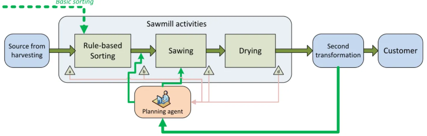
Figure 4.1: Process description

4.2 Simulation model

In order to simulate the presented basic process, as well as different log class aggregation strategies, we use agent-based simulation. The general architecture of this model is presented in Figure 4.2, which represent the basic process. However, information flows are slightly more complex to simulate the class aggregation strategies, which require log sorting to be coordinated with the production campaign.

This section first present in a general manner the model architecture, as well as the physical layout implemented. Next, it presents the log database used to simulate the delivery of input logs to be sawn. Next, the different agents and their function are described. Finally, the experimental design and the different log class aggregation strategies are presented.

(32)

Figure 4.2: Basic sawmill process model

This simulation model was built using AnyLogic, a hybrid discrete-event and agent-based simulation platform. The development of the model was inspired by a real hardwood sawmill in the province of Québec, with a reception area, a log yard and a sawmill, as described previously. Handling distances are therefore roughly equivalent to that of the real sawmill.

4.2.1 Agents’ definition

4.2.1.1 Truck agents

The truck agent is responsible to deliver logs to the sawmill. It is a simple reactive agent. Every truck agent has a similar transportation capacity. However, the mix of logs they deliver is different. In order to simulate a realistic procurement of various logs, logs are randomly chosen from the database of 1900 samples, resulting in a dynamic mix of logs for each truck arrival.

4.2.1.2 Loader agents

Next, we developed a loader agent. The loader agent has two tasks. The first task is to unload log trucks, and the second is to sort logs at the receiving area. For sorting the logs, the loader use the classification grid developed in Chapter 3. Since all the attributes are measured at the reception of the logs to know their price, we assume that once a log is valued, the grid can be simultaneously used to identify the second transformation applications that the log can be good for. According to an aggregation strategy, this application can also be merged with others to create a major group or family (see Section 4.3.3). The group is then compared with the production campaign. If the group has a positive match, the log is placed in a pile with similar logs. Otherwise, the logs are

Planning agent Sawing Drying Rule-based Sorting Second transformation Source from harvesting Sawmill activities Customer Basic sorting b c d a

(33)

placed in different piles with pre-defined groups according to the same aggregation strategy, to be used in other applications.

After this sorting process, the loader takes every pile in batch of 5 to 10 logs to pre-defined areas at the log-yard (storage area). If the sawing process feeding inventory (i.e., the feeder) is below certain level (i.e. 60 minutes of workload), logs are transported directly to the feeder instead the storage zone.

During the simulation, the loader agents are also responsible for taking the logs from the log yard and transporting them to the sawmill agent. Since all the logs has been previously classified according to a specific application or group of them, one pile becomes the principal source of logs for the sawmill during the current period (slot) according to the production campaign. Every time a feeding order is triggered (i.e. the sawmill inventory is below certain level), the loader is responsible to feed the buffer zone with logs from this pre-defined zone. If the zone has no inventory, the loader must look for logs in an alternative pile, which is chosen according to the nearest one.

4.2.1.3 Sawmill agent

Finally, we developed a sawmill agent. Like the truck agent, this agent is a simple reactive agent, which aims to emulate in an aggregated manner the sawing process. Because sawmills are currently managed to process logs in only one manner, each log leads systematically to the same mix of pieces of timber. Because logs are different, the resulting mix of timber pieces is different for each log. Therefore, we used the data from the transformation of the log sample we had in the initial database in order to create a large transformation matrix that describe the input-output relationship of the entire sample, as well as the processing time for each log according to the diameter. Consequently, the role of the sawmill agent consists in simply transforming the logs brought by the loaders into various pieces of timber.

Although in the simulation, we simulate a week of production that follows a sequence of production campaigns (i.e., a series of 1 to 3 secondary applications, see Section 4.3.2), which we refer to as a production plan, production plans do not affect the sawing agent. They only affect the loader agents, which classify the logs according to the current production campaign. These production plans are therefore exogenous parameters developed mainly to evaluate the different configurations in all possible production setting. Section 4.3.2 describes how these production

(34)

plans are generated. Next, the produced timber pieces are classified according to NHLA standard, and performance indicators are computed for comparison purpose.

4.2.2 Layout definition

As mentioned before, the current experiment was developed based on an actual sawmill in Quebec. Since the log yard is the place where all the activities happen, this becomes the layout of the experiment. This log yard is a terrain with an irregular geometry surrounding the sawmill (see Figure 4.3). In order to evaluate various log yard configurations and classification strategies, we developed several handling networks that represent each of the tested configurations. Each of these configurations was configured according to the aggregation strategies. These strategies will be described in section 4.3.4.

Figure 4.3: Layout of the computer simulation model

The next section describes the experiments carried out to evaluate the various log yard configuration and classification strategies.

(35)

4.3 Experimental design

As mentioned in Chapter 1, the specific objective of this project is to assess the performance of different levels of log class aggregation and, ultimately, to measure the value of log attributes information (see Section 1.2). In order to achieve this goal, we designed a set of experiments, which aims at emulating an extended range of production settings and evaluate all log yard configurations and classification strategies within these settings. In order to create a first reference to which every configuration can be compared to, we also develop a reference simulation model using the basic layout configuration and classification strategy. For simplification purpose, and because we only had data for yellow birch, this experimental design also only considers one single species, which represents a limit of the study. However, it is not unusual for a sawmill to process only a single species during a week of production, which is the length of the simulation horizon.

The model simulates a 5-day period, with working shift from 8AM to 5PM, two breaks of 15 minutes, and one lunch hour at noon. The modeled sawmill uses one standard loader agent at the reception area, with a maximum capacity of 15 logs per charge and one production line at the sawmill, so the production capacity of the sawmill during a work shift is only 1000 logs.

For comparison purpose, and for each simulation run, we computed the total yield, the yield of each target application, the total procurement cost of the transformed logs, the ratio between yield and cost, and finally the utilization rate of the loaders.

4.3.1 Initial log inventory

Using the distribution of the initial sample of logs used to create the different classes, we developed a random function to create three stock levels: 0, 12,000 and 24,000. According to the sawmill average output, these inventory levels represents: no inventory, two weeks and four weeks. We also classified these logs and located them in the log yard according to the considered classification strategy. This process was carried out outside the simulation horizon in order to measure only the real loader utilization during the receiving and classification process.

(36)

4.3.2 Production plan generation

Sawmills’ operations are generally organized by campaigns in a weekly manner, in order to meet the specific order for secondary transformation customers. In other words, a week is divided into at most 3 sequential campaigns of production, which represent the production plan of the week. The minimum length of a campaign is half a day, and the maximum is 5 days. Because each campaign can be set to produce timber for 1 of 7 possible types of application, there is a limited number of possible production plans. If a typical week can transform up to 3 products, the total number of scenarios is 259 (7P1 + 7P2 + 7P3). However, since the palette application has a very

low demand, no production campaign is normally allocated for this application. It is rather a by-product of the log transformation. Nevertheless, because all logs must be transformed, including low quality logs that can only produce palette timber, in our simulation model, we have allocated the last slot of the week to producing palette timber using low quality logs (i.e. Friday afternoon). Consequently, this reduces the total number of scenarios to 156 (6P1 + 6P2 + 6P3), as presented in

Figure 4.4.

Figure 4.4: Production plan possible configurations

4.3.3 Aggregation strategies

As mentioned previously, several classification strategies can be adopted with a number of class ranging between 1 class (no classification) and 7 classes. In order to design these strategies, we develop an aggregation strategy that enables us to aggregate several of the 7 classes in order to obtain fewer classes. To do so, we analyzed the database of logs and calculated the yield correlation of all classes of secondary application (see Table 4.1).

(37)

Table 4.1: Correlation matrix of logs yield in each secondary application

Floor Wardrobe Staircase Paneling Cabinet Molding Palette Floor 1.000 0.320 0.380 0.320 0.879 0.307 -0.041 Wardrobe 1.000 0.873 1.000 0.631 0.941 -0.063 Staircase 1.000 0.873 0.720 0.812 -0.040 Paneling 1.000 0.631 0.941 -0.063 Cabinet 1.000 0.594 -0.024 Molding 1.000 -0.039 Palette 1.000

Many similarities can be observed. For example, the Wardrobe, Paneling and Staircase applications have a perfect, or near perfect match, meaning that the same log can be good for one or another category among those. Along the same line, and as expected, the logs that are appropriate for these high value applications are not appropriate for lower value applications such as Palette.

In order to identify each group, we analyzed the correlation matrix and at every grouping level, we identified either the most different application from the rest of the group, or the sub-group of applications with highest correlation among them, and chose these applications to separate from the rest and create a new group. These steps are applied in the next paragraph.

4.3.3.1 Application of the aggregation strategies

Since the original grouping strategy is to have all the applications in the same group, the second one can be one group with the palette and one group with the rest of the logs. For the third strategy, we separate the applications Floor and Cabinet into a single group because they have a high correlation coefficient; we keep a separate group with the Palette, and create a third one with the rest of the applications. The fourth strategy requires removing one application from the big group (i.e. Wardrobe, Staircase, Paneling and Molding). We chose to separate the Molding and remain with the other two groups as described before (i.e. group 1: Floor and Cabinet, group 2: Palette). At this stage we realized that the first group (Floor and Cabinet) has too many logs because of the attributes of the logs in the sample, therefore for the fifth strategy we remove the

(38)

Cabinet from this group and remain with the other four as described before. For the sixth strategy we remove the Staircase from the general group so this becomes only the merge of Paneling and Molding. Finally, the seventh strategy is to have one group for each application. The previous aggregation for each strategy is presented in the Table 4.2.

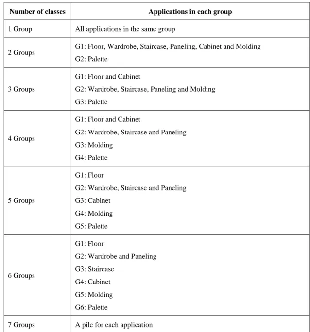
Table 4.2: Aggregation strategies

Number of classes Applications in each group

1 Group All applications in the same group

2 Groups G1: Floor, Wardrobe, Staircase, Paneling, Cabinet and Molding G2: Palette

3 Groups

G1: Floor and Cabinet

G2: Wardrobe, Staircase, Paneling and Molding G3: Palette

4 Groups

G1: Floor and Cabinet

G2: Wardrobe, Staircase and Paneling G3: Molding

G4: Palette

5 Groups

G1: Floor

G2: Wardrobe, Staircase and Paneling G3: Cabinet

G4: Molding G5: Palette

6 Groups

G1: Floor

G2: Wardrobe and Paneling G3: Staircase

G4: Cabinet G5: Molding G6: Palette

7 Groups A pile for each application

The next Section describes the different log yard layouts that were developed according these aggregation strategies.

(39)

4.3.4 Layout Strategy

Once the strategies for aggregating log classes were developed, we determine for each of them, a layout configuration to implement accordingly. Using the distribution of the log sample, and therefore the volume of logs in each category, we have designed the yard layouts as presented in the Figure 4.5.

Figure 4.5: Layout arrangement strategies

Zone 1 Sawing Pre-sorting process 2 Groups Zone 2 Pre-sorting process Zone 1 Zone 2 Sawing 3 Groups Zone 3 Zone 1 Zone 2 Zone 3 Sawing Pre-sorting process 4 Groups Zone 4 Zone 1 Zone 2 Zone 3 Sawing Pre-sorting process 5 Groups Zone 4 Zone 5 Zone 1 Zone 2 Zone 3 Zone 4 Zone 5 Zone 6 Sawing Pre-sorting process 6 Groups Zone 1 Zone 2 Zone 3 Zone 4 Zone 5 Zone 6 Zone 7 Sawing Pre-sorting process 7 Groups

(40)

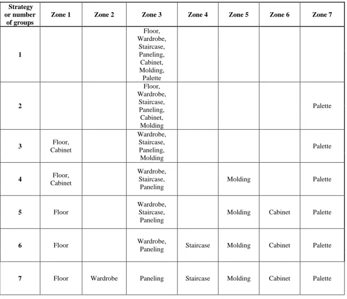
In order to match these configurations with the aggregation strategies defined in the previous section (see 4.3.3) we developed a unified grid with the defined applications per zone in the log-yard layout, as presented in Table 4.3.

Table 4.3: Aggregation strategies applied to the layout zones in the log-yard

Strategy or number

of groups

Zone 1 Zone 2 Zone 3 Zone 4 Zone 5 Zone 6 Zone 7

1 Floor, Wardrobe, Staircase, Paneling, Cabinet, Molding, Palette 2 Floor, Wardrobe, Staircase, Paneling, Cabinet, Molding Palette 3 Floor, Cabinet Wardrobe, Staircase, Paneling, Molding Palette 4 Floor, Cabinet Wardrobe, Staircase, Paneling Molding Palette 5 Floor Wardrobe, Staircase, Paneling

Molding Cabinet Palette

6 Floor

Wardrobe,

Paneling Staircase Molding Cabinet Palette

7 Floor Wardrobe Paneling Staircase Molding Cabinet Palette

Each of these 7 strategies was simulated with all 156 production plans, for a total of 1,092 combinations, with 10 replications and 3 initial stock scenarios for a total of 32,760 experiments. The results are presented and analyzed in the next Chapter.

(41)

CHAPITRE 5

RESULTS AND ANALYSIS

As mentioned in the Chapter 4, we computed for each simulation run, four key performance indicators in order to compare the general results. These performance indicators are:

1. The total first transformation yield; 2. The anticipated production yield;

3. The ratio between the anticipated yield and the total procurement cost; 4. The utilization rate of the loaders.

5.1 Output analysis

Once the results dataset were generated, they were averaged in order to analyse only one set of the ten repetitions. The 156 production plans were also analysed by considering the number of products produced (i.e. 1 to 3). Every indicator is analyzed for each aggregation strategy (i.e. 1 to 7), compared with the initial inventory level (i.e. 0, 12,000 and 24,000 logs) and with the total number of products in the production campaign (i.e. 1 to 3). The results are presented below1.

5.1.1 Total first transformation yield

The first indicator is the total first transformation yield generated for each scenario. In this case we found that when the initial inventory is zero, the total production yield is reduced when a sorting strategy is introduced. This happens because the new log sorting and handling increases loader utilization, which becomes a bottleneck (see Table 5.1 and Figure 5.1). When some initial inventory is added to the model, the sorting strategy increases this indicator to a value between 8 to 20% high. The peak yield level is reached with two piles (i.e., 2-class strategy). This suggests that only by separating the logs belonging to the Palette application, it is possible to achieve higher first transformation yields. Other strategies also exclude Palette application logs; however, they require more handling and thus, less time to process the logs.

1_{The individual tables for each indicator at every initial stock level and number of products in the production} campaign are presented in the APPENDIX D of this document.

(42)

Table 5.1: Total first transformation yield (fbm) per initial stock and strategy Strategy Initial inventory % change vs. strategy 1 Stock: 0 Stock: 12,000 Stock: 24,000 Average 1 90,878 100,162 100,231 97,090 2 83,427 123,682 141,135 116,081 20% 3 84,127 121,277 132,746 112,717 16% 4 84,052 119,579 132,386 112,005 15% 5 83,879 114,151 123,636 107,222 10% 6 83,768 112,573 119,447 105,263 8% 7 83,896 112,770 119,776 105,481 9%

Figure 5.1: Total first transformation yield (fbm) per initial stock and strategy

When analyzing the same indicator for different number of products in the production campaign, we found a similar behavior in terms of the increase of the yield when a sorting strategy is introduced (see Table 5.2 and Figure 5.2). Another finding is the increase of the total first transformation yield when several product types are treated. This improvement is because the classification strategies are more effectives in presence of a mix of products in the production plan rather than a single product, since they require predefined zones to store the products in the log yard, therefore, only one pile is dedicated to feed the sawing and thus, a shorter output is expected.

(43)

Table 5.2: Total first transformation yield (fbm) per different product types in the production campaign

Strategy Total product types in production plan % change vs. strategy 1 1 type 2 types 3 types Average

1 97,252 97,117 96,901 97,090 2 116,421 117,154 114,670 116,081 20% 3 110,105 113,343 114,703 112,717 16% 4 109,942 112,056 114,018 112,005 15% 5 106,898 106,279 108,488 107,222 10% 6 104,431 104,053 107,304 105,263 8% 7 106,027 104,394 106,022 105,481 9% Average 107,297 107,771 108,872 % Change 0.0% 0.4% 1.5%

Figure 5.2: Total first transformation yield (fbm) for different product types in the production campaign

5.1.2 Anticipated production yield

The anticipated production yield is the volume of timber produced in each campaign (for the corresponding application). In other words, it is the anticipated yield of the secondary transformation achieved by each sorting strategy. In this indicator, we found that the scenario with no initial inventory has no relevance since no remarkable change is observed when the

(44)

sorting strategies are introduced. Nonetheless, in presence of some initial inventory, the anticipated volume of secondary transformation products rises 28% in average, meaning a high performance of the classification techniques (see Table 5.3).

Table 5.3: Average anticipated production yield (fbm) for every strategy and inventory level

Strategy Initial inventory % change vs strategy 1 Stock: 0 Stock: 12,000 Stock: 24,000 Average 1 26,102 28,933 28,991 28,009 2 25,718 37,678 43,777 35,724 28% 3 25,998 38,519 43,879 36,132 29% 4 26,063 38,599 44,086 36,249 29% 5 25,899 38,192 41,446 35,179 26% 6 25,890 37,428 41,847 35,055 25% 7 25,827 37,557 41,032 34,806 24%

Figure 5.3: Average anticipated production yield (fbm) for every strategy and inventory level

Consequently with this finding, the anticipated production yield is affected in similar proportion when compared with different product types in the production campaign (see Table 5.4and Figure 5.4). Again, the indicator shows that the use of sorting strategies has a better performance in presence of a mix of products in the production plan, with an average increase of 2.9% when three product types are transformed instead of one.