HAL Id: hal-00536953
https://hal.archives-ouvertes.fr/hal-00536953
Preprint submitted on 19 Nov 2010
HAL is a multi-disciplinary open access
archive for the deposit and dissemination of
sci-entific research documents, whether they are
pub-lished or not. The documents may come from
teaching and research institutions in France or
abroad, or from public or private research centers.
L’archive ouverte pluridisciplinaire HAL, est
destinée au dépôt et à la diffusion de documents
scientifiques de niveau recherche, publiés ou non,
émanant des établissements d’enseignement et de
recherche français ou étrangers, des laboratoires
publics ou privés.
Dynamic identification of a 6 dof industrial robot
without joint position data
Maxime Gautier, Alexandre Janot, Pierre-Olivier Vandanjon
To cite this version:
Maxime Gautier, Alexandre Janot, Pierre-Olivier Vandanjon. Dynamic identification of a 6 dof
in-dustrial robot without joint position data. 2010. �hal-00536953�
M. Gautier*, A. Janot**, P.O. Vandanjon***
* Université de Nantes, IRCCyN, 1, rue de la Noë - BP 92 101 - 44321 Nantes Cedex 03, France. ** HAPTION S.A, Atelier Relais de Soulgé Route de Laval, 53210 Soulgé sur Ouette, France
*** Laboratoire Central des Ponts et Chaussées, Route de Bouaye BP 4129, 44341Bouguenais Cedex, France
Abstract: Off-line robot dynamic identification methods are mostly based on the use of the inverse dynamic model,
which is linear with respect to the dynamic parameters. This model is sampled while the robot is tracking reference trajectories that excite the system dynamics. This allows using linear least-squares techniques to estimate the parameters. This method requires the joint force/torque and position measurements and the estimate of the joint velocity and acceleration, through the bandpass filtering of the joint position at high sampling rates. A new method called DIDIM has been proposed and validated on a 2 degree-of-freedom robot. DIDIM method requires only the joint force/torque measurement. It is based on a closed-loop simulation of the robot using the direct dynamic model, the same structure of the control law, and the same reference trajectory for both the actual and the simulated robot. The optimal parameters minimize the 2-norm of the error between the actual force/torque and the simulated force/torque. A validation experiment on a 6 dof Staubli TX40 robot shows that DIDIM method is very efficient on industrial robots.
1. INTRODUCTION
The usual identification method based on the Inverse Dynamic Identification Model (IDIM) and least-squares (LS) technique has been successfully applied to identify inertial and friction parameters of several robotic prototypes and industrial robots (M. Gautier 1986)(Ha et al. 1989) (M. Gautier 1997)(Swevers et al. 2007)(Wisama Khalil & Dombre 2002), amongst others. Good results can be obtained provided a well-tuned derivative bandpass filtering of joint position to calculate the joint velocities and accelerations is used.
The Direct and Inverse Dynamic Identification Model (DIDIM) method needs only the joint force/torque measurements (M Gautier et al. 2008). It is based on a closed-loop simulation using the direct dynamic model while the optimal parameters minimize the 2-norm of the error between the actual force/torque and the simulated force/torque, assuming the same control law. This non-linear least-squares problem is dramatically simplified using the inverse dynamic model to formulate the simulated force/torque as an algebraic function linear in relation to the parameters. This paper recalls the DIDIM method and gives new experimental results obtained using a 6 dof robot. The paper is organized as follows: section 2 reviews the usual identification technique of the dynamic parameters of the robot. Section 3 presents the DIDIM method. The modelling of the TX40 industrial robot is presented in section 4. The experimental results are given in section 5. Finally, section 6 is the conclusion.
2. IDIM: INVERSE DYNAMIC IDENTIFICATION MODEL TECHNIQUE
The inverse dynamic model (IDM) of a rigid robot composed of n moving links calculates the motor torque vector τidm, as a function of the generalized coordinates and their
derivatives. It can be obtained from the Newton-Euler or the Lagrangian equations (Wisama Khalil & Dombre 2002). It is given by:
= ( ) + ( , )
idm
τ M q q N q q (1)
Where q, q and q are respectively the
nx 1
vectors of generalized joint positions, velocities and accelerations,( )
M q is the
n nx
robot inertia matrix, and N q q( , ) is the
nx 1
vector of centrifugal, Coriolis, gravitational and friction forces/torques. The modified Denavit and Hartenberg notation allows to obtain a dynamic model that is linear in relation to a set of standard dynamic parameters, χst (M. Gautier 1986):
idm st st
τ IDM q,q,q χ (2)
Where ID Mst
q, q, q
is the
n Nx s
jacobian matrix of τidm, with respect to the
Nsx1
vector χst of the standard parameters given by T T T T ... 1 2 n st st st st : T j j st XXj XY XZ YY YZ ZZ M X M Y M Z M Ia Fv Fcj j j j j j j j j j j j off (3)where:XX , XY , XZ , YY , YZ , ZZj j j j j j are the six components of the inertia matrix of link j at the origin of frame j. M X , M Y , M Z j j j are the components of the first moment of link j. Mj is the mass of link j, Iaj is a total inertia moment for rotor and gears of actuator j. Fvj,
j
Fc are the viscous and Coulomb friction parameters of joint
j.
j off
is an offset parameter.
The base parameters are the minimum number of dynamic parameters from which the dynamic model can be calculated. They are obtained from the standard inertial parameters by
regrouping some of them by means of linear relations (M Gautier 1991). The minimal inverse dynamic model can be written as:
idm
τ ID M q,q,q χ (4)
ID M q, q, q is the
n bx
matrix of the minimal set of basis functions of the rigid body dynamics, (5)χ is the
b 1x
vector of the b base parameters.Because of perturbations due to noise measurement and modeling errors, the actual force/torque differs from τidm
by an error, e, such that:
idm
τ e IDM q,q,q χ e
(6)
Equation (6) represents the Inverse Dynamic Identification Model (IDIM). We consider the off-line identification of the base dynamic parameters χ, given measured or estimated off-line data for τ and
q , q , q
, collected while the robot is tracking some planned trajectories.
q , q , q
in (6) are estimated with
ˆq, q, q ˆ ˆ
, respectively, obtained by bandpass filtering the measure of q (M. Gautier 1997).The actual force/torque, τ is calculated by :
τ = gτ vτ (7)
where v is the
n 1x
control signal vector calculatedaccording to the control law and g , is the
nxn
diagonalmatrix of the drive gains.
The inverse dynamic identification model (IDIM) (6) is sampled at a frequency measurement fm, at different times
k
t , k1,...,nm, while the robot is tracking a reference trajectory
q , q , qr r r
, during the time length Tobs, of the trajectory.We obtain an over determined linear system of n T* obs* fm
equations and b unknowns such that:
fm fm fm
ˆ ˆ ˆ
Y τ W q,q,q χ ρ (8)
In order to window the identification frequency range into the model dynamics, a parallel decimation procedure lowpass filters in parallel Yfm and each column of Wfm and resamples them at a lower rate, keeping one sample over nd. We obtain:
ˆ ˆ ˆ
Y τ W q,q,q χ ρ (9)
where: Y τ
is the (rx1) vector of measurements, built from the actual force/torque τ. W
q, q, qˆ ˆ ˆ
is the (rxb) observation matrix, built from the estimated values
ˆq,q,q ˆ ˆ
of
q , q , q
.ρ is the (rx1) vector of errors. r=n*nm/nd is the number of
rows in (9). In Y and W, the equations of each joint are grouped together such that:
1 T
n T T
1 T
n T TY Y ... Y ,W W ... W
(10)
Yj and Wj represent the nm/nd equations of joint j. The
ordinary LS (OLS) solution ˆχ minimizes ρ. Using the base parameters and tracking “exciting” reference trajectories (M. Gautier & W. Khalil 1992), we get a well conditioned matrix W. The LS solution ˆχ is given by:
1
T T ˆχ W W W Y W Y (11) Standard deviations i ˆ , are estimated under the assumptions that W is a deterministic matrix and ρ, is a zero-mean additive independent Gaussian noise, with a covariance matrix Cρρ, such that:
T 2
ρρ ( ) σρ r
C E ρρ I (12)
E is the expectation operator and Ir, the rxr identity matrix.
An unbiased estimation of the standard deviation is:
2 2
ρ
σ (r b )
ˆ Y W χˆ (13)
The covariance matrix of the estimation error is given by:
T 2 T 1 χχ [( )( ) ] σ (ρ ) ˆ ˆ ˆ ˆ ˆ C E χ χ χχ W W (14) i 2 χ χχ σˆ C (ˆ ˆ i ,i) is the i th
diagonal coefficient of Cχχˆ ˆ. The
relative standard deviation
ri χ % σˆ is given by: ri i χ χ i % σˆ 100 σˆ χˆ , for χˆi ≠ 0 (15)
The OLS can be improved by taking into account different standard deviations on joint j equations errors (M. Gautier 1997). Each equation of joint j in (9), (10), is weighted with the inverse of the standard deviation of the error calculated from OLS solution of the equations of joint j , given by:
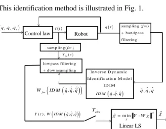
j j j j j ˆ ˆ ˆ Y τ W ID M q ,q ,q χρ (16)This identification method is illustrated in Fig. 1.
Robot In v e rse D yn a m ic Id e n tific a tio n M o d e l ID IM ˆ ˆ ˆ ID M q , q , q q q qˆ , ,ˆ ˆ
fm ˆ ˆ ˆ W ID M q ,q ,q Linear LS 2 ˆ m in Y-W ˆˆ ˆ ( ), , , Y W ID M q q q q t ( )t Control law ˆ q ,q ,qr r r obs T sam p lin g ( ) b an d p ass filterin g fm lo w p ass filterin g + d o w n sam p lin g sa m p lin g (fm ) fm Y τFig. 1. IDIM LS identification scheme.
3. DIDIM: DIRECT AND INVERSE DYNAMIC IDENTIFICATION MODEL TECHNIQUE
3.1 Theoretical approach
DIDIM (M Gautier et al. 2008) is a closed loop output error (CLOE) method which does not require joint position data.
The output, y=τ, is the actual joint force/torque τ, and the simulated output ys=τddm, is the simulated joint force/torque.
τddm, is the force/torque input of the Direct Dynamic Model
(DDM) which can be obtained by writing the IDM equation (1), as following:
( ddm, ) ddm = ddm - ( ddm, ddm, )
M q q τ N q q (17)
Where M q( ddm, ) and N q( ddm, qddm, ) depend on an
estimation of the base parameters χ.
The signal qddm(t, χ), is the result of the integration of the
linear implicit differential equation. The optimal solution, ˆ , minimizes the quadratic criterion, J(χ) = ||Ys–Y||2.
Y τ and YS
τd d m
are vectors obtained by filtering anddownsampling the vectors of samples of the actual force/torque τ, and of the simulated force/torque τddm,
respectively.
This non-linear LS problem is solved by the Gauss-Newton regression. It is based on a Taylor series expansion of ys, at a
current estimate ˆχk
, of the parameters at iteration k:
+1 +1 k k k k k S S ˆ S ˆχ ˆ y ( χ ) y ( χ ) y ( χ ) / χ χ χ o (18)
y ( χ ) /S χ
ˆχk is the (nxb), jacobian matrix of ys, withrespect to χ, evaluated at ˆχk. The input force/torque of the
DDM, τddm, can be calculated with the analytical expression
of the inverse dynamic model (4), such as:
s ddm idm ddm ddm ddm
y χ τ χ τ χ ID M q χ ,q χ ,q χ χ (19) Then the jacobian matrix is given by:
k k k S d d m id m ˆ ˆ ˆ χ χ χ k k k k d d m d d m d d m y χ χ χ ˆ ˆ ˆ ˆ ID M q ( χ ),q ( χ ),q ( χ ) χ χ (20)Because of the same closed loop control for the actual and for the simulated robot (see section B), the simulated position, velocity and acceleration have little dependence onχ . Then
k k k
d d m ˆ d d m ˆ d d m ˆ
ID M q ( χ ),q ( χ ),q ( χ ) ID M q ,q ,q for any k
ˆχ ,
and the jacobian matrix (20) can be approximated by:
k S k k k d d m d d m d d m ˆχ y ˆ ˆ ˆ ID M q ( χ ),q ( χ ),q ( χ ) χ (21)Taking the approximation (21) of the jacobian matrix into the Taylor series expansion, it becomes:
k k k
k+ 1 ddm ˆ ddm ˆ ddm ˆ
y ID M q ( χ ),q ( χ ),q ( χ ) χ oe (22)
This is the Inverse Dynamic Identification Model, IDIM, (6), where
q , q , q
are estimated with
qddm, qddm, qddm
, simulated from (17). At each iteration k, the IDIM method is applied as described in section 2. The sampling of (22) at a sampling rate fm, gives the over-determined linear system:
, k
fm fm d d m d d m d d m ˆ fm
Y τ W q ,q ,q χ ρ (23) The parallel decimation of (23) gives:
d d m d d m d d m,ˆk
Y τ W q ,q ,q χ χρ (24)
The LS solution of (24) calculates ˆχk1 , at iteration k+1. This process is iterated until:
k1 k
/ k to l1tol1 is a value ideally chosen to be a small number to get fast
convergence with good accuracy.
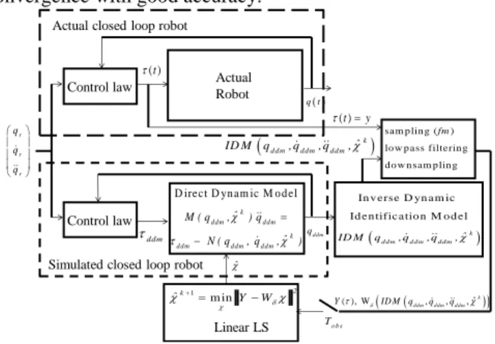
r r r q q q Actual Robot D irect D yn am ic M o d el k d d m d d m k d d m d d m d d m ˆ M ( q , ) q ˆ N ( q , q , ) Linear LS +1 m in 2 k ˆ Y W ( )t Control law ˆ ˆ ( ), W , , , k ddm ddm ddm Y ID M q q q o b s T ddm q t Control law In v e rse D yn a m ic Id e n tific a tio n M o d e l k d d m d d m d d m ˆ ID M q ,q ,q , k d d m d d m d d m ˆ ID M q ,q ,q , ( )t y ddm q
Actual closed loop robot
Simulated closed loop robot
sam p lin g ( ) lo w p ass filterin g d o w n sam p lin g
fm
Fig. 2. DIDIM, with the Gauss-Newton regression, identification scheme.
Because this method uses both models DDM and IDIM, it is named the DIDIM method: Direct and Inverse Dynamic Identification Models technique. The DIDIM method with the Gauss-Newton regression is illustrated Fig. 2.
3.2 Initialization of the algorithm
A problem with non linear optimization algorithm is how to choose the initial values ˆχ0
. We propose an algorithm not sensitive to the initial conditions, which assumes that the condition
qddm( χ ), qˆk ddm( χ ),qˆk ddm( χ )ˆk
q ,q ,q
, is satisfied at any iteration k , starting with k=0. This is possible by taking the same control law structure for the actual robot and for the simulated one with the same performances given by the bandwidth, the stability margin or the closed-loop poles. Because the simulated robot parameters, ˆχk, change at each iteration k, the gains of the simulated control law must be updated according to ˆχk
.
For example, let us consider a PD control law for each joint j. The inverse dynamic model IDM (1) for the joint j, can be written as a decoupled double integrator perturbed by a coupling force/torque, such that:
= ( )
j
j idm j , j j j
τ τ M q q p (25)
pj is considered as a perturbation given by:
( ) ( , ) n j j ,i i j i j p M q q N q q
(26)Mj,i(q) which depends on q , is approximated by a constant
inertia moment Jj, given by:
( )
j j
j j a j , j j a q
Jj, is the maximum value, with respect to q, of the inertia
moment around joint zj axis. This gives the smallest damping
value and the smallest stability margin of the closed-loop second order transfer function, while q varies. It must be taken at least as ZZj + Iaj, which can be calculated from a
priori CAD values. The joint j dynamic model is approximated by a double integrator, where pj, is a
perturbation, as following:
( )
j j j j , j j j j
q τ p / M q τ p / J
(28)
Let us consider the joint j PD control of the actual robot which is illustrated Fig. 3:
+ - +- j a g j r q j a v k a1 j J 1 s 1 s ++ j a p k j p j v j qj qj qj ap j ap j J g
Fig. 3. Joint PD control of the actual robot. The joint j , force/torque is given by:
j j
a j g v
(29)
Where agtj is the actual drive gain, aJj is the actual value of Jj, apJ
jand apgtj are a priori values of the actual unknown values a
Jj and a
gtj, respectively.
If a priori values are equal to the actual ones, akpj and akvj are
the PD control gains of the normalized double integrator system 1/s2. The closed-loop performances are chosen with the desired 2 poles of the second order closed-loop transfer function characterized by, dωnj, dζj, where dωnj is the desired
natural frequency which characterizes the closed-loop bandwidth, dζj is the desired damping coefficient which
characterizes the closed-loop stability margin. It comes:
2 j a d d p nj j k / , j a d d v j nj k 2 (30)
Now, let us consider the joint j PD control of the simulated robot which is illustrated Fig. 4.
+ - +- j a p g j r q j a v k 1 s 1 s ++ j s p k ddm j p j ddm v ddm j q qddm j ddmj ddm j q ap j ap j J g 1 k j ˆ J k j ap j ˆ J J
Fig. 4. Joint PD control of the simulated robot.
The variables
,
j j j j j
ddm ddm ddm ddm ddm
v , q , q , q , in Fig. 4, are computed by numerical integration of (17). The control law of the simulated robot has the same structure as the actual one, Fig. 3. It can be seen that the actual gain
j a ap ap v j j k J / g must be multiplied by k a p j j ˆ
J / J in order to obtain the same normalized double integrator open-loop system 1/s2 and the same closed-loop transfer function. The proportional gain,
j s
p
k , does not depend at all on the parameters values, but the derivative gain in the simulator must be updated with k
j ˆ J , at each iteration k. This allows to keep
qddm( χ ), qˆk ddm( χ ),qˆk ddm( χ )ˆk
q ,q ,q
, at each iteration k.We propose to take a regular inertia matrix 0
( ddm,ˆ )
M q , in order to have a good initialization for the numerical integration of the DDM. It can be obtained with:
0 0 ˆ , except for, 0 1, j Ia j1, n (31)
The inertia of the rotor and gear of actuator j is generally taken into account in the IDM model (1) as τ
j
r Ia jqj.
Then, the initial inertia matrix becomes the identity matrix, which is the best regular matrix:
0 ( ddm,ˆ ) = n
M q I (32)
Another point is to choose the state initial condition of the state vector,
qddm(0), qddm(0)
, in order to integrate the DDM. Because DIDIM doesn't need the joint position measurement, the actual values
q(0), q(0)
, are supposed tobe unknown and we choose,
qddm(0), qddm(0)
qr(0), qr(0)
, which is close to
q(0), q(0)
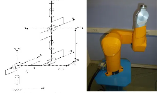
. Because the closed-loop transient response due to different initial conditions differs between the actual and the simulated signals during a transient period of approximately, 5/dωn, the corresponding joint force/torquesamples are eliminated from the identification data in (23). 4. CASE STUDY: MODELLING OF THE TX40 ROBOT The Stäubli TX-40 robot has a serial structure with six rotational joints. The robot kinematics is defined using the modified Denavit and Hartenberg notation (Fig. 5).
The geometric parameters defining the robot frames are given in Table 1. The parameter j = 0, means that joint j is
rotational, αj and dj give respectively theangle and distance
between zj-1 and zj along xj-1, whereas j and rj give
respectively theangle and distance between xj-1andxjalong
zj. Since all the joints are rotational then jis the position
variable of joint j.
Fig. 5. Link frames of the TX-40 robot
Table 1 Geometric parameters of the TX-40 robot
j σj αj dj θj rj 1 0 0 0 θ1 0 2 0 -π/2 0 θ2 0 3 0 0 d3 = 0.225m θ3 rl3 = 0.035m 4 0 π/2 0 θ4 rl4 = 0.225m 5 0 -π/2 0 θ5 0 6 0 π/2 0 θ6 0
The TX40 robot is characterized by a coupling between the joints 5 and 6 such that 5 5
6 6 qr K 5 0 q qr K 6 K 6 q . Where qr jis the
velocity of the rotor of motor j, qjis the velocity of joint j,
K5 is the transmission gain ratio of axis 5 and K6 is the
transmission gain ratio of axis 6. Thus, the duality relation of force/torque gives 5 5 6 6 c r c r K 5 K 6 0 K 6 . Where, τcj is the
motor's torque of joint j, taking into account the coupling effect, τrj is the electro-magnetic torque of the rotor of motor
j. The coupling between joints 5 and 6, also adds to the effect
of the inertia of rotor 6 and new viscous and Coulomb friction parameters fvm6and fcm6 to both τc5 and τc6.
We can write: sign( )
5 c 5 Ia q6 6 fvm q6 6 fcm 6 q6 and sign( ) 6 c 6 Ia q6 5 fvm q6 5 fcm 6 q5 .
Where τ5, τ6 already contain the terms
j j j j j j
( Ia q fv q fc sign( q )) , for j=5 and 6 respectively,
2 2
5 5 5 6 6
Ia K Ja K Ja and 2
6 6 6
Ia K Ja (33)
Jaj is the moment of inertia ofrotor j, fvm6, fcm6 are the friction
parameters due to the coupling between joints 5 and 6. The TX40 has Ns=86, standard dynamic parameters given by
the 14*6 usual standard parameters (3), plus fvm6and fcm6.
For IDIM-LS method, we use the standard inverse dynamic model (2). The columns of the matrix ID Mst
q, q, q
in (2) can be obtained using the recursive algorithm of Newton-Euler. We use the software SYMORO+ to automatically calculate the customized symbolic expressions of the models (Wisama Khalil & Dombre 2002). The base parameters χ and the minimal model (4) are automatically calculated using aQR numerical method (M Gautier 1991). The matrices
( ddm, )
M q and N q( ddm, qddm, ) are numerically calculated using the IDM model (1), τidm( , q q , q ) , for special values of
,
q q , q .
5. EXPERIMENTAL RESULTS
The identification of the dynamic parameters has been carried out using one trajectory using the controller CS8C of the Stäubli robots. The joint positions and torques are stored with a sampling frequency measurement fm=5KHz. The IDIM-LS
off-line estimation is carried out with a filtered position ˆq,
calculated with a 50Hz cut-off frequency forward and reverse Butterworth filter, and with the velocities ˆq, and the accelerations, qˆ , calculated with a central difference algorithm of ˆq. The parallel decimation of Yfmand Wfm, in
(8), is carried out with a sample rate divided by a factor,
nd=100, and a lowpass filter cut-off frequency equal to,
0.8*fm/(2*nd)=20Hz. There are 60 base parameters which can
be simplified to 23 well identified essential parameters with good relative standard deviation.
The DIDIM method is initialized with all the standard parameters equal 0 except Iaj=1, j≠5and Ia5=2, due to the
coupling effect (33). The simulation is carried out with the actual stored reference trajectory and the CS8C controller of the TX40, with updating the gains with k a p
j j
ˆ
J / J , and using the simulink software.
A step of DIDIM takes 7' on a 2008 working station PC computer. The results are given in Table 2.
Table 2: DIDIM Estimation after 2 step
Parameter ˆ1 r χ % σˆ Parameter ˆ1 % σχˆr ZZ1R 1.30 0.65 Fv3 2.37 1.2 Fv1 8.71 0.8 Fc3 6.6 2.0 Fc1 7.69 2.5 Ia4 0.029 5.0 XX2R -0.53 3.6 Fv4 1.0 1.2 XZ2R -0.16 7.2 Fc4 2.47 2.2 ZZ2R 1.09 0.8 Ia5 0.053 12.0 MX2R 2.11 0.4 Fv5 2.52 2.3 Fv2 7 1.1 Fc5 2.77 5.0 Fc2 7.74 1.7 Fv6 0.72 2.7 ZZ3R 0.14 3.7 Fc6 0.9 8.0 MY3R -0.64 1.8 fvm6 0.8 2.4 Ia3 0.083 7.1 fcm6 1.6 4.4
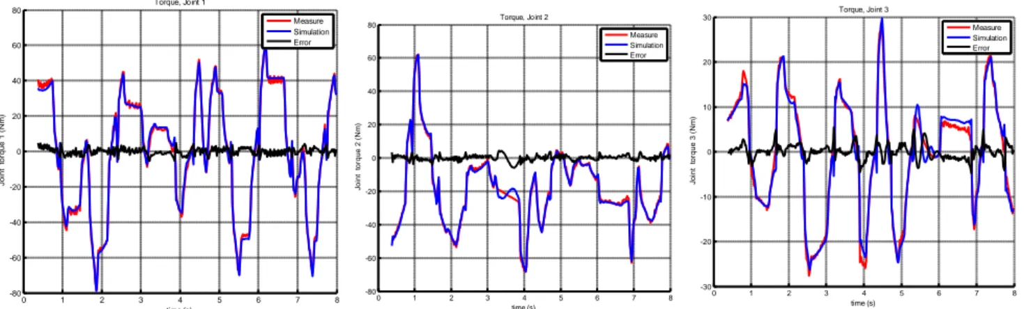
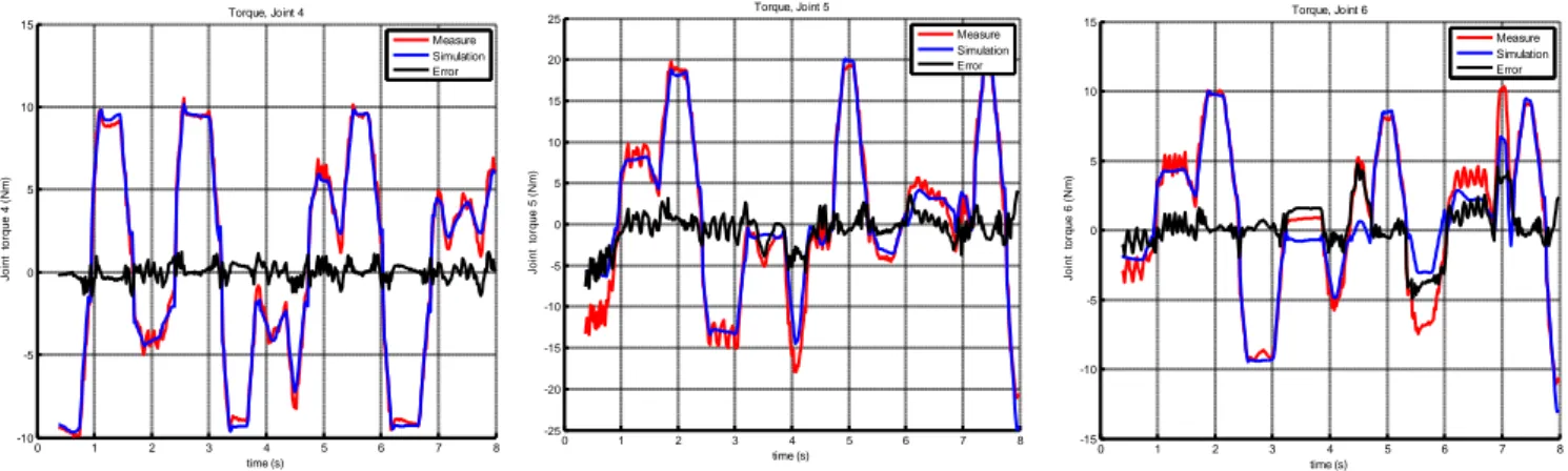
It needs only 1 step to obtain the optimal solution which is very close to the IDIM solution. Hence, the DIDIM method has a very fast convergence. A validation is plotted on Fig. 6, at the decimated frequency 50Hz. It shows that the actual joint torques, Y(τ), and the torques estimated with the identified model, Ye W
qddm,qddm,qddm,ˆ1
ˆ1, as defined in (24) are very close. Both methods, IDIM-LS and DIDIM, give a small relative norm error, Y Wˆ / Y <3%, which shows a good accuracy for the model and for the identified value. 0 1 2 3 4 5 6 7 8 -80 -60 -40 -20 0 20 40 60 80 time (s) Jo in t t o rq u e 1 ( N m ) Torque, Joint 1 Measure Simulation Error 0 1 2 3 4 5 6 7 8 -80 -60 -40 -20 0 20 40 60 80 time (s) Jo in t t o rq u e 2 ( N m ) Torque, Joint 2 Measure Simulation Error 0 1 2 3 4 5 6 7 8 -30 -20 -10 0 10 20 30 time (s) Jo in t t o rq u e 3 ( N m ) Torque, Joint 3 Measure Simulation Error0 1 2 3 4 5 6 7 8 -10 -5 0 5 10 15 time (s) Jo in t t o rq u e 4 ( N m ) Torque, Joint 4 Measure Simulation Error 0 1 2 3 4 5 6 7 8 -25 -20 -15 -10 -5 0 5 10 15 20 25 time (s) Jo in t t o rq u e 5 ( N m ) Torque, Joint 5 Measure Simulation Error 0 1 2 3 4 5 6 7 8 -15 -10 -5 0 5 10 15 time (s) Jo in t t o rq u e 6 ( N m ) Torque, Joint 6 Measure Simulation Error
Fig. 6. DIDIM, validation, red line: actual torque, blue line: estimated torque,
, 1
1 e d d m d d m d d m ˆ ˆ Y W q ,q ,q . n cm_jnts [t qdg_drv] vcmd [t q_drv] pfbk [t qg_drv] pcmd ratio_inertie* u invred* u invred* u invred* u invred* u red'* u red* u red'* u kt' [t cm_drv] cm_drv MATLAB Function calcul_qdd MATLAB Function calcul_n [t atc_drv] atc [t qddg_drv] acmd z 1 cm-n q q qd 1 s 1 s q_jnts qdd_jnts qd_jnts qdg_jnt qg_jnt q_jnt ts cm_drvs cm_jnt ecm_jnt qddg_jnt cm_jnts atcr_drvs, A qdd_drvrs, rd/s/s qdr_drvs, rd/s qr_drvs, rd q_drvs, rd Icmd_drvs, A Commande STARC1 Clock 6 6 6 6 6 6 6 6 6 6 6 6 6 6 6 qd 6 6 6 6 6 q 12 6 6 6 6 6 6 6 6 6 6 cm-n 12 6 6 6 6 6 6 6 6 6 6 6 6 6 6 6 6 6Fig. 7. Simulation of the TX_40 with simulink, red line: CS8C controller, black line: the direct dynamic model. 6. CONCLUSION
This paper deals with a new off-line identification technique of robot dynamic parameters, called DIDIM for Direct and Inverse Dynamic Identification Models technique. This method is a closed-loop Output Error approach, considering the output is the joint force/torque. The optimal parameters are the solution of a non-linear least-squares problem which is solved with a Gauss-Newton method. Each step of the iterative procedure of the Gauss-Newton regression is dramatically simplified to a linear regression which is solved with the Inverse Dynamic Identification Model technique (IDIM). In this paper we prove that DIDIM is very efficient on a 6 dof industrial robot, with a 1 step convergence starting with a regular initialization of the parameters.
REFERENCES
Gautier, M., 1991. Numerical calculation of the base inertial parameters.
Journal of Robotics Systems, 8(4), 485-506.
Gautier, M., Janot, A. & Vandanjon, P., 2008. DIDIM: A new method for the dynamic identification of robots from only torque data. In Proc.
of IEEE International Conference on Robotics and Automation.
2008 IEEE International Conference on Robotics and Automation. Pasadena, California, USA, pp. 2122-2127. Available at: [Accessed October 1, 2009].
Gautier, M., 1997. Dynamic Identification of Robots with Power Model. In
Proc. of IEEE International Conference on Robotics and
Automation. IEEE International Conference on Robotics and
Automation (ICRA). Albuquerque, USA, pp. 1922-1927. Gautier, M., 1986. Identification of Robot Dynamics. In Proc. of IFAC
Symposium on Theory of Robots. IFAC Symposium on Theory of
Robots. Vienne, Austria, pp. 351-356.
Gautier, M. & Khalil, W., 1992. Exciting trajectories for the identification of the inertial parameters of robots. International Journal of
Robotics Research, 11(4), 362-375.
Ha, I., Ko & Kwon, 1989. An efficient estimation algorithm for the model parameters of robotic manipulators. IEEE Trans. on Robotics and
Automation, 5(6), 386-394.
Khalil, W. & Dombre, E., 2002. Modeling identification and control of
robots, Taylor and Francis.
Swevers, J., Verdonck, W. & De Schutter, J., 2007. Dynamic model identification for industrial robots - Integrated experiment design and parameter estimation. IEEE control systems magazine, 27(5), 58-71.