Multi-Robot Navigation and Cooperative Mapping in a Circular Topology
Texte intégral
Figure


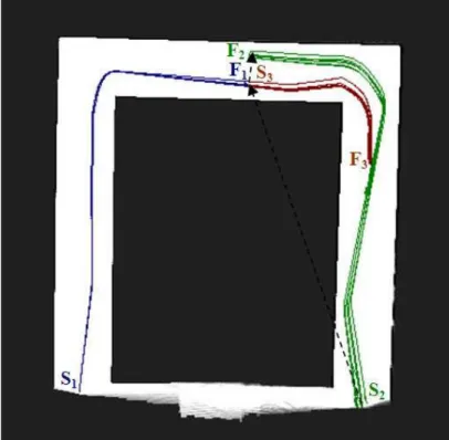
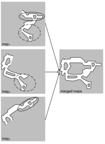
![Figure 2.10: Example of a map of the Freiburg University campus constructed with the SLAM-algorithm proposed in [17]](https://thumb-eu.123doks.com/thumbv2/123doknet/12388012.330904/29.892.130.754.123.584/figure-example-freiburg-university-campus-constructed-algorithm-proposed.webp)
Documents relatifs
[r]
Vous pouvez aussi rejoindre l’un des nombreux GROUPES associés, ou le quitter si un ami vous y a inclus et qu’il ne vous convient pas (beaucoup l’ignorent, mais il est
When solving this monitoring problem, we apply a decoupling strategy to decompose the problem into two subproblems: one is to select suitable robots and quickly move
Our objectives were: first, to explore if interpersonal motor coordination impairments already shown during interactions with a human partner 20,21 also apply to interactions with
All this is very classical and studied, but the fact that the robot must interact for a long time with the human introduces a new challenge: how a machine can be acceptable for
When the assignment and the routing problems are solved, the residual problem can be modelled as a two-stage hybrid flow shop with maximal time lags where the machine in
La dualité Tannakienne pour les réseaux Tannakiens donne une équivalence entre C(X/S) ◦ et la catégorie des représentations localement libres d’un schéma en groupes G(X/S) affine
• We suggest a simulation framework in which path planning, path following, and collision avoidance collaborate to detect and resolve conflicts between their strategies (Section 5)..
