HAL Id: hal-01462577
https://hal.archives-ouvertes.fr/hal-01462577
Submitted on 6 Jun 2020
HAL is a multi-disciplinary open access
archive for the deposit and dissemination of sci-entific research documents, whether they are pub-lished or not. The documents may come from teaching and research institutions in France or abroad, or from public or private research centers.
L’archive ouverte pluridisciplinaire HAL, est destinée au dépôt et à la diffusion de documents scientifiques de niveau recherche, publiés ou non, émanant des établissements d’enseignement et de recherche français ou étrangers, des laboratoires publics ou privés.
agri-environmental schemes
Maria Espinosa-Goded, Pierre Dupraz, Jesus Barreiro-Hurlé
To cite this version:
Maria Espinosa-Goded, Pierre Dupraz, Jesus Barreiro-Hurlé. Fixed costs involved in crop pattern changes and agri-environmental schemes. [University works] auto-saisine. 2009, 31 p. �hal-01462577�
Fixed costs involved in crop pattern changes
and agri-environmental schemes
Maria ESPINOSA-GODED, Pierre DUPRAZ, Jesùs BARREIRO-HURLÉ
Working Paper SMART – LERECO N°09-15
September 2009
UMR INRA-Agrocampus Ouest SMART (Structures et Marchés Agricoles, Ressources et Territoires) UR INRA LERECO (Laboratoires d’Etudes et de Recherches Economiques)
Fixed costs involved in crop pattern changes and agri-environmental
schemes
Maria ESPINOSA-GODED
Área de Economía y Sociología Agrarias (AESA), Instituto de Investigación y Formación Agraria y Pesquera (IFAPA), Granada, Spain
Pierre DUPRAZ
INRA, UMR1302, F-35000 Rennes, France
Agrocampus Ouest, UMR1302 SMART, F-35000 Rennes, France
Jesùs BARREIRO-HURLÉ
Área de Economía y Sociología Agrarias (AESA), Instituto de Investigación y Formación Agraria y Pesquera (IFAPA), Granada, Spain
Auteur pour la correspondance / Corresponding author Pierre DUPRAZ
INRA, UMR SMART
4 allée Adolphe Bobierre, CS 61103 35011 Rennes cedex, France
Email: [email protected] Téléphone / Phone: +33 (0)2 23 48 56 06 Fax: +33 (0)2 23 48 53 80
Fixed costs involved in crop pattern changes and agri-environmental schemes Abstract
Agri-environmental schemes are the main policy instrument currently available in the European Union to promote environmentally friendly farming practices. Nevertheless, the adoption rate of these measures is still limited. This paper develops a profit maximizer theoretical framework to explain the farmer’s sign-up decision and the area to put under an agri-environmental measure characterised by a change in the crop pattern. The application concerns an agri-environmental measure awarding the introduction of alfalfa in cereal farms in Natura 2000 designated areas of Aragon (Spain). The econometric specification accounts for both the upper censoring of the enrolled area, constrained by the available eligible area, and the self-selection of contractors according to the extra-profit of their enrolment. To test the absence of fixed costs of enrolment, a simple tobit with a lower and an upper bound, that corresponds to the non fixed costs situation, is compared to the censored model with selection. Estimated specifications based on the enrolled area do not provided normally distributed residues and are not suitable to carry out the likelihood ratio test. Estimated specifications based on the share of enrolled area in the eligible area provide normally distributed residues. The likelihood ratio test rejects the absence of fixed costs. Technical factors as well as social capital variables are taken into consideration as determinants of technical and transaction costs. Estimation results show that there is an adoption barrier derived from the know-how affecting the fixed compliance costs of introducing the new crop. In addition, there is an adoption barrier derived from transaction costs which are reduced in the presence of social networks. These results suggest that a non linear payment mechanism or auctions might be suitable to ensure a better coverage of Natura 2000 eligible areas by the contracts, with a limited increase in related public expenditures.
Keywords: agri-environmental scheme, land use, fixed costs, transaction costs,
qualitative and limited dependent variable model
Revoir les primes agri-environnementales: l’impact des coûts fixes dans la participation aux programmes agri-environnementaux
Résumé
Les programmes agri-environnementaux constituent l’un des principaux instruments de promotion de pratiques agricoles favorables à l’environnement dans l’Union Européenne. Cependant, le taux d’adoption de ces mesures reste souvent limité. Ce papier vise à expliquer l’adoption d’une mesure modifiant l’assolement. Un modèle d’allocation de la surface de l’exploitation agricole, supposée fixe, est basé sur la maximisation de la somme des profits des différentes cultures, potentiellement affectés par des coûts fixes relativement à la surface cultivée. L’application empirique concerne l’introduction de luzerne dans des exploitations céréalières situées en zones Natura 2000 en Aragon (Espagne). Le programme offre une prime de 102€ par hectare de surface céréalière convertie à la luzerne. La spécification économétrique, correspondant à une forme particulière de tobit généralisé, prend en compte simultanément la censure à droite de la surface contractualisée par la surface éligible de l’exploitation et l’auto-sélection des contractants en fonction de la variation du profit total liée au contrat, qui constitue la deuxième variable dépendante. L’analyse micro-économique permet de montrer qu’en l’absence de coûts fixes liés à la contractualisation, la spécification économétrique se réduit à un tobit simple. La surface sous contrat est alors la seule variable à expliquer. Elle est toujours censurée à droite par la surface éligible, mais aussi à gauche en zéro. En l’absence de coûts fixes, la variable latente correspondant à la surface sous contrat est en effet redondante avec la variation du profit liée au contrat, dont elle est la duale pour une prime donnée. L’estimation des tobit simple et généralisé permet de tester simplement l’absence de coûts fixes liés à la contractualisation. Ensuite, la comparaison des déterminants de l’adoption d’une part et de la surface sous contrat d’autre part permet d’identifier partiellement la source et la nature de ces coûts fixes. Certains sont clairement liés à des investissements en savoir-faire lié à la luzerne, d’autres sont des coûts de transaction spécifiques à l’adoption du contrat. Les résultats suggèrent qu’un paiement non linéaire ou des mécanismes d’enchères permettraient de mieux couvrir les zones à enjeux sans trop accroître la dépense publique.
Mots-clefs : mesures agri-environnementales, allocation de la terre, coûts fixes, coûts
de transaction, modèle à variables qualitatives et à variables dépendantes limitées
Fixed costs involved in crop pattern changes and agri-environmental schemes
1. Introduction
Agri-environmental schemes (AES) are the main policy instrument currently available in the European Union (EU) to foster improvements in the relationship between agriculture and the environment. Over 35 million hectares were under some kind of AES in the EU-15 in 2003 with an overall 3.7billion € in public funds being allocated annually to this policy and an overall expenditure of 14 billion € of EAGGF funds during the 2000-2006 period (DG Agriculture, 2006). Payment levels for each AES are calculated based on supply side approaches, aiming at compensating forgone profits and additional costs (article 39-4, Regulation 1698/2005). Formerly, under Agenda 2000, a 20% incentive was foreseen in some cases, this option has been removed for the current programming period although transaction costs, if necessary, can also be compensated for.
Prior research has identified that premiums based on forgone profit might not be sufficient to ensure farmer participation. Cooper and Signorello (2008) show how risk-related issues can require premiums to cover more than the mean loss in profit associated with adoption. They back their theoretical assumption estimating this additional payment comparing contingent valuation estimates of willingness to accept with actual forgone profits. Additionally Barreiro-Hurlé et al. (2008) have shown that the sign-up decision is not solely affected by farm technical characteristics, thus identifying the limited effect of premiums in fostering adoption, especially for low requirement measures. These results point at the fact that even the 20% incentive was not sufficient to foster AES sign-up, thus partially explaining the low enrolment rates detected throughout the EU for AES. While Austria, Finland and Luxembourg have more than two thirds of their national utilised agricultural area (UAA) involved in agri-environmental measures, in Belgium, Denmark, Greece, the Netherlands and Spain the coverage is just a mere 5% of their total UAA (Glebe and Salhofer, 2007).
This paper expands the understanding of the effect of supply side estimated premiums in AES participation, considering the potential effects of fixed costs associated with sign-up. Several studies have considered factors influencing farmers’ participation. They can be categorised in four main categories (Vanslembrouck et al., 2002),
(food and environment demand) characteristics constitute the so-called extrinsic factors while farm (size, crop portfolio, etc.) and individual farmer (age, education, etc.) characteristics are intrinsic factors. Fixed costs related to adoption would be related to costs that do not vary with the amount of area enrolled and are mainly related with investments (both assets and know-how) needed to implement AES. An additional source of fixed costs can be transaction costs (TC), which are increasing with asset specificity. Assets are specific when they are sunk, i.e., not profitable in another transaction. Therefore actions and warrants needed to secure the transaction entail TC which themselves are sunk. There is empirical evidence that AES requiring higher specific assets involve higher TC, and that some TC do not depend on the enrolled area: they are fixed costs (Ducos and Dupraz, 2007). Logically, such fixed TC should accompany fixed costs of specific assets. One special case of these costs is related to AES promoting a change in the crop pattern. Fixed costs are also related to variable costs and benefits because higher investment or specialization of the farmer implies higher land profitability, inducing a higher loss when the crop is removed. This paper tests whether fixed costs do exist for AES implementation. The empirical study also examines what types of fixed costs are significant. Are they related to TC only? Are they generated by specific investments? The results therefore provide evidence on whether the current approach to set premiums levels is adequate to foster adoption of this type of schemes.
The paper is structured as follows: section 2 presents the conceptual framework with the theoretical model adapted to test the research hypothesis. Section 3 includes a description of the AES selected for corroborating the theoretical hypothesis as well as the field work undertaken and the estimated econometric model. Next, section 4 presents the model estimation results and section 5 provides a summary of the main findings and the policy recommendations derived from them.
2. Conceptual framework
Profit maximising farmers face the option to sign-up or not an AES contract. AES adoption is thus based on an increase in land profitability derived from a change in practices or land allocation. A simplified two activity model is developed, where activity c is the current land use and activity a the alternative land use that will be subsidized by the AES. The farm profit structure is defined as to consider the effects of
fixed costs associated either with current or alternative land management, and transaction costs associated with AES implementation. In this static model, we assume that fixed costs are sunk costs, considering that the costs of the physical assets, that can be resold or rented on the market, are adjusted on a per-hectare basis and integrated into the variable profit function. So the fixed costs which are specific to each land use typically include specific knowledge costs, part of the costs of specific equipment or land improvement that cannot be recovered on the second hand markets or rented at fair prices.
2.1. Costs and benefits with and without an AES contract
Before the AES introduction, the land allocation model is based on the profit maximising program [1]. Farmers’ face a surface restriction in which the total eligible area (ST) is allocated between the two competing options, current production (Sc), and the alternative production (Sa). All areas are positive, implying that the area of any land use i (Si) cannot exceed ST.
T a a T c C T a T a a a C T C T c c c S S S S S S Z FC Z S p Z FC Z S p
Max
a ; 0 ); ( ) , , ( ) ( ) , , ( 2 1 [1]Profit is split into two components: the first one (C1) is associated with current production and the second one (C2) with the alternative production. For each land use i, specific fixed costs (FCi) are considered. Fixed costs are assumed to be totally explained by the fixed factors endowments of the farm (ZT). They are different from zero only if the area devoted to the related production is strictly positive. In this case, their amount does not depend on this area. Each production variable profit ( ) i depends on the variable input-output prices (pi), on the area under cultivation (Si) and on fixed factors endowments (ZT). Individual variable profit functions are assumed to be increasing and quasi concave with respect to the area allocated to the corresponding land use. The profit in the initial situation is the solution of program [1], denoted
) (Sa*
To gain understanding of the effect of fixed costs on sign-up decision, two initial situations are considered: one where land use a existed before AES implementation and one where it did not. The situation where the land use a already covers the whole eligible area should not be relevant as the AES aims at promoting this land use.
If land use a already covered a part of the farm, the land allocation equilibrium before AES implementation implies that fixed costs are covered for both crops and that marginal returns are equal. Equation [2] comes from the first order condition of programme [1], where Sa* is the optimal area for land use a. It is necessary that the marginal profit (is) of one of the land uses decreases with its area for the existence of
such an interior solution.
)
(
)
(
* a a* s a T c sS
S
S
With c
ST Sa*
FCc and a
Sa* FCa [2]In the other initial situation, there is no area for land use a that provides a higher profit than land use c, which is summarized by expression [3].
0 ) ( ) ( ) ( a a a a C a T c C T c S FC S FC S S FC S [3]
With the introduction of the AES, the profit maximisation program [4] includes a third component (C3), in addition to the two components of program [1]. It is made of the AES payment (Sa), assuming a constant per-hectare payment, minus the fixed and
variable TC associated to the AES contract, respectively denoted FTC and VTC. Variable transaction costs (VTC) are assumed to be increasing and quasi-convex when the area of the alternative crop increases. These TC potentially depend on fixed factors endowments (ZT). They also depend on social capital variables (ZSC) which distinguish them from technical costs and benefits.
2 1 ) ( ) , , ( ) ( ) , , ( C T a T a a a C T C T a T c c S Z FC Z S p Z FC Z S S pMax
a
T a C SC T a SC T a FTC Z Z VTC S Z Z S S S ( , ) ( , , ); 0 3 [4]If land use a already covered a part of the farm, the AES contract is adopted and it displaces the initial equilibrium (equation [2]) to S* AES if the change in variable profit (P) due to the contract covers the AES related fixed transaction costs FTC. Other fixed costs, associated with each crop technology, remain unchanged in the new allocation of land, because both crops were already grown before contracting. The marginal profits for land use a and c reach a new equilibrium according to the AES premium and the marginal transaction cost function (VTCs). If the premium is high enough to exceed the difference in marginal profits for the whole eligible area, the enrolled area covered by crop a is constrained by this eligible area. Relation [5] provides the characteristics of the solutions of programme [4] when the AES contract is adopted. If the change in variable profit (P) does not exceed the fixed transaction costs FTC, the contract is not accepted and equations [2] still hold. The fixed technology costs (FCi) do not matter since they were already covered by the variable profit in the initial situation.
sc(ST Sa*AES) sa(Sa*AES) or cs(0) sa(ST) FTC S VTC S S S S S S S P AES a s AES a a a AES a a a T c AES a T c ) ( . ) ( ) ( ) ( ) ( * * * * * * [5]
If land use a was not present on the farm before AES implementation, the fixed technology costs of the crop a matter. The contract is signed-up if the change in variable profit (P) due to the contract covers both the fixed transaction costs FTC and the fixed technology costs FCa (relationship [6]). Again, the total eligible area may restrict the enrolled area, with a premium exceeding the difference in marginal profits between current and alternative crop for this area. Otherwise the premium equals the difference in marginal profits for the optimal enrolled area.
S S
S
S
S VTC S FCa FTC P AES a s AES a AES a a T c AES a T c ) ( * * * * [6]Fixed costs related to the land use c are not taken into account, because they do not change with the reduction of this land use area. Even if the land use c completely disappears because of the AES contract, the related fixed costs are not recovered as we assume they are sunk.
Graph 1 illustrates the change in variable profit (P) due to the contract, when the crop a is initially absent. VTCs are supposed to be negligible. Fixed costs are not represented. Decreasing marginal profits are represented. From the left to the right, the marginal profit of crop a decreases as its area increases while the marginal profit of crop c increases as its area decreases. Three possible outcomes are illustrated on Graph 1: 1. The change in the variable profit due to the contract (P represented by the area ABC on the graph) is not high enough to cover the fixed costs for the optimal enrolled area with a contract corresponding to A. So the contract is not signed.
2. The change in the variable profit (P represented by the area DBE on the graph) is high enough to cover the fixed costs for the optimal enrolled area (S*AES) with a contract corresponding to D. So the contract is signed. This is an internal equilibrium, where the premium is equal to the difference in the marginal profits between the two land allocations.
3. The premium is higher than the marginal profit difference and P is higher than the additional fixed costs. In this case the enrolled area is limited by the eligible area. The unrestricted profit maximising enrolled area would be higher than the eligible area.
Graph 1: Land allocation between two crops (cereal and alfalfa)
Source: Own elaboration
The graph does not represent every possible individual situation of the farmers facing the AES contract. On the one hand, the contract may be refused even if the unrestricted enrolled area exceeds the eligible area. It happens when the change in the variable profit P for the enrolled area equalling the eligible area does not cover the additional fixed costs due to the contract. On the other hand, the contract may be refused when there are no fixed costs at all. It happens if the premium does not cover the difference in the marginal profits of crop c and a for any positive enrolled area. It means that the unrestricted optimal enrolled area would be negative. The existence of fixed costs and the type of fixed costs are empirical issues. In order to reveal non negligible fixed costs, it is necessary to consider the econometric specifications with and without fixed costs.
2.2. Modelling the farmer’s decision with and without fixed costs
The empirical analysis is based on the preceding theoretical results. Accordingly, we assume that the observed enrolled area is the optimal enrolled area (S*AES) for each farm. A strictly positive enrolled area is observed when the profit with the contract exceeds the profit without the contract. As the profit with the contract depends on the
AES
2 a
AES
1 a
AES
3 a
S
TS
*AES c
AES a
PROFIT CONTRACT (P) NOT CONSIDERING FC A E B D C
optimal enrolled area, we first consider the notional enrolled area (S*) that is not bounded by zero or the eligible area. S* is the solution of program [4] without the area restrictions (0Sa ST) and always verifies the first order condition [7].
*) ( *) ( *) (ST S as S VTCs S c s [7]
S* does not depend on fixed costs. It only depends on the marginal cost and profit curves and on the AES premium. Referring to equation [4], S* depends on the prices of current and alternative crops and on the farm and farmer characteristics (ZT, ZSC).
If there are no fixed costs, the value of the notional area S* both determine the decision to sign the contract and the enrolled area S*NF according to the decision rules [8]. If the notional area is negative, meaning that the premium does not compensate the difference in marginal profits for any strictly positive enrolled area, the contract is not signed and the enrolled area is zero. If the notional area exceeds the eligible area ST, the enrolled area equals the eligible area. In between, the enrolled area equals the notional area.
) , , , , ( * ) , , , , , ( (.) * 0 ) , , , , , ( ) , , , , ( * 0 ) , , , , , ( 0 ) , , , , ( * * * * SC T a c SC T a c T NF T T SC T a c T NF T SC T a c SC T a c T NF SC T a c Z Z p p S Z Z p p S S S S S Z Z p p S S S Z Z p p S Z Z p p S S Z Z p p S [8]
When fixed costs are not negligible, the participation in AES depends on the difference in total profits with and without contract. A strictly positive enrolled area is observed when this difference is strictly positive only. The profit without contract is simply the profit of the initial situation((Sa*)). The profit with contract is the profit obtained with the optimal area S*NF, denoted (S*NF) in relationship [9]. Indeed, the optimal area does not depend on fixed costs and the relationship [8] still holds, however the total profit assuming that the contract is signed-up (S*NF) includes fixed costs.
FTC FC FC S VTC S S S S S a c NF s NF NF a NF T c NF * * * * ( * ) [9]The difference in total profits with and without contract is denoted D(Sa*,S*NF). It depends on the initial situation as explained in the preceding section. If the alternative land use already existed before the AES introduction, the related fixed costs (FCa) are already covered by the variable profit; if it did not, the fixed costs have to be covered by the change in variable profit derived from the contract (equations [10]).
FTC S VTC S FC S S S S S S D S FTC S VTC S S S S S S S S S D S NF s NF a NF a T c NF T c NF a a NF s NF a a NF a a T c NF T c NF a a ) * ( * * * * , 0 ) * ( * * * * , 0 * * * * * * [10]Equations [10] confirm that the difference in profits can never be strictly positive when S*NF equals zero, because Sa* maximises the profit without contract. They also show that the contract might not be profitable because of fixed costs, despite a strictly positive S*NF in contrast with the situation without fixed costs. A strictly positive enrolled area is observed if and only if the contract is profitable, meaning that the variable profit (P) covers the fixed costs (relationships [3] and [4]). There are two sub-cases: the enrolled area reached the eligible area and the enrolled area equals the notional area. With fixed costs, the decision rules are provided by equations [11]. The enrolled area simultaneously depend on the notional area S* defined by [7] and on the difference in total profits, in contrast with [8]. The notional area S* does not depend on the eligible area, while D(Sa*,S*NF) does because of S*
NF
. Other exogenous determinants are prices, AES premium and fixed characteristics of farm and farmers as in [8].
) , , , , ( * ) , , , , , ( (.) * 0 0 (.) ) , , , , , ( ) , , , , ( * 0 ) , , , , , ( 0 ) , , , , , ( 0 ) , , , , , ( * * * SC T a c SC T a c T AES T T SC T a c T AES T SC T a c T SC T a c SC T a c T AES T SC T a c Z Z p p S Z Z p p S S S S D S Z Z p p S S S Z Z p p S S Z Z p p D Z Z p p S S S Z Z p p D [11]
If the difference in total profits is negative, the contract is not adopted and the enrolled area S*AES is zero whichever the values of S* and S*NF. In particular the notional area S* may reach the eligible area ST without providing a change in the variable profit that is large enough to cover the fixed costs. Moreover, the smaller the eligible area is, the lower the probability that the change in total profits is positive, if all other determinants are the same. For a strictly positive difference in total profits, there are two possible results: the notional area is always strictly positive but may or may not reach the eligible area.
A last analytical result is important for the empirical analysis. If the fixed costs FTC and FCa both equal zero, the decision rules [8] and [11] are equivalent. In this case S*NF is the solution of program [4]. This means that a strictly positive notional area S* implies a strictly positive D(Sa*,S*NF).
2.3. Econometric specifications with and without fixed costs
Limited and qualitative dependent variable econometrics enable the estimation of the dependent variables D and S* according to their exogenous determinants
) , , , , ,
( ST pc pa ZT ZSC , as far as a sample of AES participants and non participants is available. The observed variables are the dummy variable Y, that indicates AES participation, and the observed enrolled area S which is the profit maximising enrolled area (S *AES). Referring to [11], the two observed dependent variables respectively correspond to the dependent latent variables D and S* according to [12].
T SC T a c T SC T a c T SC T a c T T T SC T a c T SC T a c T SC T a c S S Z Z p p S S Y S Z Z p p S S Z Z p p S D S S Y S Z Z p p S S Z Z p p D S Y S Z Z p p D , 0 ) , , , , ( * 1 ) , , , , , ( * 0 0 ) , , , , , ( 1 ) , , , , ( * 0 ) , , , , , ( 0 0 0 ) , , , , , ( [12]We assume that the latent variable pair (D , S*) is distributed according to a binomial normal cumulative function. The deterministic part is a linear function of the explanatory variables of vector X that gathers a constant term and the observed determinants )(,ST,pc,pa,ZT,ZSC . The subscript j refers to the observation j for each variable while Greek letters are the parameters to be estimated. The observations are assumed independently and identically distributed. The sample likelihood is calculated with the cumulative function of the reduced and centred normal distribution, 2 the cumulative function of the reduced and centred binomial normal distribution and 2 the corresponding joint density function of the binomial normal distribution. Referring to [12], there are three types of observations: non participants, participants whose enrolled area reaches the eligible area, and participants with an enrolled area that does not reach the eligible area. Accordingly the sample likelihood (L(.)) is provided by [13].
Tj j j j Tj j j j S S Y j X u u i j S S Y j Tj i j Y j j j j j i j j j du X S u S X X X X S Y L X X N S D ; 1 / / 2 ; 1 / 2 0 / 2 2 ) ), / ( , ( . ) , / ) ( , / ( . ) / ( 1 ) , , , , , , , ( , , , , * , [13] The parameters
, ,
and
are then estimated by the maximum likelihood estimator. As the latent variable D is not observed, apart from its sign, the parameter cannot be identified. It is normalised to 1. This econometric specification of S corresponds to a generalised tobit in which strictly positive values of S are selected by Y, with a right censoring of S by ST.
When the fixed costs FTC and FCa both equal zero, we noticed that the decision rules [8] and [11] are equivalent. As a consequence, the variable D is redundant with S* and Y is redundant with S which is censored by zero on the left and censored by ST on the right, as shown by the relationships [14].
T SC T a c T SC T a c T SC T a c T T T SC T a c T SC T a c SC T a c T SC T a c S S Z Z p p S S Y S Z Z p p S S Z Z p p S D S S Y S Z Z p p S S Z Z p p D S Y Z Z p p S S Z Z p p D , 0 ) , , , , ( * 1 ) , , , , , ( * 0 0 ) , , , , , ( 1 ) , , , , ( * 0 ) , , , , , ( 0 0 0 ) , , , , ( * 0 ) , , , , , ( [14]The sample likelihood is calculated with the cumulative function of the reduced and centred normal distribution, and the corresponding density (equations [15]).
Tj j Tj j j S S j i j S S j Tj i S j j j j j i j X S S X X X S Y L X N S 0 / / 0 / 2 ) / ( . ) / ) ( . ) / ( 1 ) , , , , ( , * [15]If fixed costs are negligible, the results of the generalised tobit [13] and the results of the simple tobit [15] must be the same as far as the same explanatory variables (X) are used in both estimations. Significantly different results would contradict the hypothesis of negligible fixed costs. The negligible fixed costs hypothesis is equivalent to the restriction (, )=( , 1), which can be tested by the likelihood ratio test. If Ls and Ps respectively denote the likelihood and the number of parameters of the simple tobit [15]
and if Lg and Pg respectively denote the likelihood and the number of parameters of the generalised tobit [13], the statistic T=2[log(Lg)-log(Ls)] follows a Chi-square distribution with (Pg-Ps) degrees of freedom.
3. Case study
A survey of eligible farmers for an alternative crop AES has been carried out. This AES measure1 requires rain-fed land allocation to alfalfa against a per-hectare payment of 102€. The farmers are free to decide how much land they enrol. The contractors are the farmers who enrolled some land into the measure and the non contractors are the farmers who did not. Both types of farmers were surveyed. The replacement of cereal crops by alfalfa is expected to have positive effects on the biologic diversity in the targeted Natura 2000 areas where eligible land has been designated. The AES eligible land is the non permanent rain fed crop land. This measure can be considered as a high-asset specificity measure due to the change in the crop pattern, requiring additional know-how and an opportunity cost due to the loss of cereal output when alfalfa harvest is not ensured due to weather variability. Fieldwork has been undertaken in three counties in Aragón (Northern Spain). There were 107 contractors only, resulting in an uptake rate of 2.8%. So the sample was discretionally allocated to over-represent contractors (40% of the questionnaires were addressed to contractors). The total sample contains 157 farmers among which 62 enrolled land into the scheme2. The 94 non contractors were randomly selected from the different municipalities according to their overall percentage of eligible farmers. The survey revealed that 53 non contractors were not aware of the AES and had not considered their opportunity of applying for an AES contract. As a consequence, these 53 observations were removed from our analysis. Indeed we assume rather well informed farmers who are able to calculate their profit with and without contract. One contractor was also removed because of inconsistent and missing answers to the questionnaire. The usable sample is reduced to 103 farmers with 61 contractors and 42 non contractors. Eligible and enrolled areas in this sample are
1
A detailed description of the measure requirements can be found in BOA (2005).
2
Differences between total sign-ups (107) and interviewed farmers (62) are due to same farm-holding applying for more than one contract (two cases), contact data not facilitated by the managing authority (36 cases) or farmer not willing to participate in the survey (seven cases).
described in Table 1. The eligible area does not differ significantly between contractors and non contractors. The average enrolled area of contractors is 21 hectares, and reaches a maximum of 100 hectares for three of them. Ten farmers enrolled their whole eligible area. According to our model we assume they would have enrolled a larger area if possible.
Table 1: Eligible and enrolled area in the sample
Total sample Descriptive statistics eligible area (ha) enrolled area (ha) enrolled share (%) 103 farmers average 74.44 12.68 26 max 562.00 100.00 100 min 0.09 0.00 0
Participants Descriptive statistics eligible area (ha) enrolled area (ha) enrolled share (%) 61 farmers average 77.70 21.42 45 max 562.00 100.00 100 min 3.50 3.00 4
The questionnaire used was designed by the research team after a thorough review of previous research, agricultural structure in the area and interviews with the AES managing authority. An initial version was field tested with 5 farmers for comprehension before generating the final version. The survey was conducted during the period April-June 2007 by a market research company, which employed interviewers with agronomic background and trained in situ by the research team. The final version of the questionnaire gathered data regarding three main topics: a) farm basic data, b) information channels, knowledge and networks of the farmer and c) AES eligible and enrolled areas3.
3
Table 2 presents the variables used to measure the different concepts put forward in the microeconomic model, the economic values of farmers’ behaviour they are supposed to affect and their expected sign on the adoption decision. Table 3 presents the differences in the frequencies of these variables between contractors and non contractors and the related independence Chi2 tests. Contractors have more frequently livestock on their farms and grew more frequently dry alfalfa before the AES introduction, while non contractors are more frequently specialised in dry cereal crops and owners of harvesters. At this stage, the other variables do not discriminate contractors and non contractors significantly.
Table 2: Selected explanatory variables, affected values and expected impact on AES sign-up Variable Description Affected values Expected impact
eliarea Eligible area (number of ha) and FCa a
+
spedrycer Non-irrigated cereal specialization farmer (1 if yes)4
c
-
irrcereal Crop distribution includes irrigated cereal (1 if yes)
c
-harvester Farm owns harvester (1 if yes) c -
dryalfalfa Farm already had alfalfa before AES (1 if
yes) FCa +
irralfalfa Crop distribution includes irrigated alfalfa (1 if yes)
a
and FCa +
ZT
livestock Presence of livestock on the farm-holding (1 if yes)
a
and FCa +
cooperative Farmer is a member of a cooperative for agri-input provision (1 if yes)
c
, , FTC, a
VTC
- and +
formation
Farmer attended agricultural formation courses during the last five years (1 if yes)
c
, , a
FTC, VTC
+
infaesfinen Farmer obtains information related to AES
from financial entities (1 if yes) FTC, VTC +
ZSC
addinfsource Farmer uses more than one source for
technical advice (1 if yes) FTC, VTC +
4
This variable is constructed assuming specialization implies the farm has a non-irrigated cereal area above the mean of farms with this land use (58 ha). Results are robust with regards to alternative specialization measures (i.e. area above the third quartile).
Table 3: Selected explanatory variables, differences between contractors and non contractors
Variable Contractors Non contractors p-value of Chi-2 test
eliarea 77.7 ha 69.7 ha 0.5059 spedrycer 21% 48% 0.0049 irrcereal 26% 50% 0.0135 harvester 3% 19% 0.0079 dryalfalfa 54% 21% 0.0009 irralfalfa 34% 34% 0.7126 ZT livestock 67% 33% 0.0007 cooperative 69% 76% 0.4158 formation 57% 48% 0.3293 infaesfinen 13% 5% 0.1594 ZSC addinfsource 20% 17% 0.6992 4. Results
The first step of the econometric analysis is the choice of the econometric specification. We estimated the generalised tobit with sample selection of contractors and a right censoring of the enrolled area corresponding to the likelihood given by [13]. The maximum likelihood estimator was computerised with the QLIM procedure of the SAS software. Estimations with two alternative specifications have been carried out. In the first one, the dependent variables are the dummy indicating the AES enrolment and the enrolled area, which is censored upward by the eligible area. In the second one, the dependent variables are the dummy indicating the AES enrolment and the share of the enrolled area in the eligible area, which is censored upward by 1. This second specification, using the share of the enrolled area in the eligible area as a dependent variable, is simply described by the relationships [12] to [15] where Sj* is replaced by
T j S
S */ , S by j S /j ST and ST by 1. As the variable addinfsource is never significant, results are presented without it. Both specifications bring similar results regarding the explanatory variable effects in the generalised tobit estimation (Annex 1). However the assumption of a normal distribution of the enrolled area residues is rejected according to the Kolmogorof-Smirnoff or other goodness of fit tests, while it is not rejected when the share of the enrolled area in the eligible area is the dependent variable (see Annex 2). As a consequence, we use the second specification to carry out the likelihood ratio test. It is based on the results of the generalised tobit and of the simple tobit displayed in Table 4.
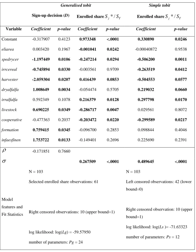
Table 4: Comparison of the generalised tobit with the simple tobit results
Generalised tobit Simple tobit
Sign-up decision (D) Enrolled share
T j S
S */ Enrolled shareSj*/ST
Variable Coefficient p-value Coefficient p-value Coefficient p-value
Constant -0.317907 0.4123 0.973348 <.0001 0.330890 0.0246 eliarea 0.003420 0.1967 -0.001041 0.0242 -0.00040872 0.9538 spedrycer -1.197449 0.0106 -0.247214 0.0294 -0.506200 0.0011 irrcereal -0.745894 0.0330 -0.003561 0.9709 -0.263519 0.0412 harvester -2.059304 0.0207 0.416439 0.0853 -0.504553 0.0577 dryalfalfa 1.008649 0.0034 -0.054474 0.5705 0.219032 0.0660 irralfalfa 0.592349 0.1078 0.216379 0.0128 0.297798 0.0170 livestock 0.690225 0.0349 -0.286717 0.0047 0.029561 0.8072 cooperative -0.477363 0.2037 -0.203472 0.0220 -0.299589 0.0217 formation 0.759415 0.0345 -0.096700 0.2853 0.098844 0.4046 infaesfinen 1.753722 0.0133 -0.149401 0.2696 0.225690 0.2391
-0.171851 0.7660
0.267509 <.0001 0.489645 <.0001 Model features and Fit Statistics N = 103Selected enrolled share observations: 61
Right censored observations: 10 (upper bound=1)
log likelihood: log(Lg) = -59.57950 number of parameters: Pg = 24
N = 103
Left censored observations: 42 (lower bound=0)
Right censored observation: 10 (upper bound=1)
log likelihood: log(Ls )= -71.63323 number of parameters: Ps = 12
The statistic T=2[log(Lg)-log(Ls)] equals 24.10746.
So, the probability that the hypothesis (, )=( , 1) is true is lower than 5% according to our data set. As a consequence, we can reject the hypothesis of negligible fixed costs.
The comparison of sign-up decision and enrolled share determinants in the generalised tobit helps to identify the determinants of fixed costs and the determinants of variable costs. The variables which are significant for the sign-up decision and do not influence the enrolled area affect more the fixed costs than the variable costs of contracting. Namely dryalfalfa, formation and infaesfinen clearly decrease fixed costs of contracting while irrcereal increases such costs. As infaesfinen is assumed to affect transaction costs only, its significant effect shows that some fixed costs are transaction costs. Some variables affect the share of enrolled area and the sign-up decision accordingly. It means that they have an effect on the variable costs of contracting. spedrycer and cooperative negatively affect the area under contract, probably because they positively affect the cereal variable profit. Accordingly, spedrycer discourages the sign-up decision; cooperative also does but not significantly. We cannot conclude from these results whether spedrycer or cooperative affect fixed costs. In contrast, irralfalfa positively affects the area under contract, probably because it positively affects the alfalfa variable profit. Accordingly, irralfalfa almost significantly favours the sign-up decision. We cannot conclude from these results whether irralfalfa affects fixed costs.
The cases of livestock and harvester deserve further discussion, because they have opposite effects on the sign-up decision and on the enrolled share. Clearly, farmers with livestock have lower fixed costs associated with the introduction of alfalfa, however their marginal profit of enrolled land decreases faster than for farmers without livestock: undertaking a comparative analysis between farmers with and without livestock shows that farmers with livestock have smaller holdings and, correspondingly less eligible surface. harvester discourages AES uptake. According to our model, this is explained by a positive effect of harvester on the cereal marginal profit, for instance by realising size economies as farms owing their harvester are the largest ones. The positive effect of harvester on the enrolled share is more difficult to understand. Referring to Annex 1, we can see that harvester seems to have the expected negative effect on the enrolled area. So, its positive effect on the share of the enrolled area in the eligible area might be explained by the interplay of the eligible area, which is larger for farms with harvester, and the economies of size due to the harvester that are larger for largest farms with
largest eligible areas than for relatively smaller farms with harvester that accordingly enrol a larger share of their eligible land.
Some information regarding the nature of the fixed costs associated with this AES can be obtained from a detailed analysis of individual variables. Social capital variables, which are significant for the adoption and are not for the enrolled area, would reflect that fixed costs are not only technical in nature but include transaction costs. Moreover technical variables describing the presence of irrigated cereal impede adoption, while the presence of alfalfa before the scheme favours adoption and it does not influence on the area enrolled, therefore identifying the crop management know-how as a potential source of fixed costs.
5. Summary and policy implications
The results support that the adoption decision for the selected AES is influenced by the existence of fixed costs related to AES participation. Fixed costs in this case are explained both by technical and social capital variables, involving both technical and transaction costs. Only a part of fixed costs are purely related to the agri-environmental scheme mechanism that requires information transfer and processing as well as administrative work. So the agri-environmental scheme is the opportunity to reveal the fixed costs associated to the introduction of a new crop, by studying the behaviour of eligible farmers. These results are obtained with an econometric specification that is fully in line with the microeconomic analysis of the farmland allocation. The estimated model simultaneously accounts for both the upper censoring of the enrolled area, constrained by the available eligible area, and the self-selection of contractors according to the extra profit of their enrolment.
Factors defining the marginal profitability of land affects the adoption decision, influencing negatively adoption when cereal crop is considered and positively under the alternative crop, alfalfa. Specialized cereal growers with higher marginal profitability of land due to an investment in fixed costs (like the harvester) or the presence of irrigated cereal are less willing to apply for the AES as it is less profitable to change the crop pattern. On the other hand farmers with livestock that can graze on the alfalfa and therefore obtain a profit or farmers with the presence of irrigated alfalfa on their farm and with an easier access to inputs are more willing to participate. Sources of fixed
costs are identified by variables influencing the decision to enrol adoption without affecting the enrolled area. Technical fixed costs are related to the know-how management of the new crop, represented by the previous cultivation of this crop. Fixed costs are also influenced by social capital variables (formation and farmers well connected to financial entities). These variables do not affect marginal profits of any of the crops, directly. Accordingly they reveal the existence of fixed transaction costs. Reported results are in line with those by Ducos and Dupraz (2007) which identify the constraints involved by specific investments regarding the AES compliance costs. In our case, more technically demanding measures such as those which imply a change in the crop pattern seem to highlight the role of fixed technical costs, making such measures less profitable and adopted than measures where only marginal costs are at stake.
If new AES promoted under the rural development plan for 2007-2013 in the EU want to follow a “deep and narrow” approach (i.e. very specific measures with demanding crop and management changes) current legislative framework can be a barrier for success. Compensating for transaction costs might not suffice to ensure enrolment, as fixed technical costs can be independent of transaction costs and curtail sign-up through a negative effect on marginal profitability. Moreover, other strategies to increase adoption, such as promotion of social networks to ensure more efficient information dissemination and reduction in transaction costs, albeit necessary, would not solve this problem if technical fixed costs are relevant.
The use of market-based mechanism, such as contract auctions (Latacz-Lohman and Van der Hamsvoort, 1997) could overcome this deficiency as bids posted by farmers would be covering all cost concepts related to AES implementation. For standard contracts, non linear payments, associating a lump sum payment and a per hectare payment for instance, may increase participation and enrolled areas without increasing the exchequer cost too much.
References
Barreiro-Hurlé J., Espinosa-Goded M., Dupraz P. (2008). Does intensity of change matter? Factors affecting adoption in two Agri-Environmental Schemes. Poster presented at the 107th European Association of Agricultural Economists (EAAE) Seminar “Modelling Agricultural and Rural Development Policies”. 30 January, Seville, Spain.
BOA (2005). Orden de 27 de Septiembre de 2005, del Departamento de Medio Ambiente, por la que se establecen los requisitos y ámbito de aplicación de parte de las ayudas agroambientales gestionadas por el Departamento de Medio Ambiente para el año 2006. Boletín Oficial de Aragón n. 125 (21/10/2005).
Cooper J., Signorello G. (2008). Farmer premiums for the voluntary adoption of conservation plans. Journal of Environmental Planning and Management, 51(1): 1-14.
DG Agriculture (2006). Rural Development in the European Union: Statistical and Economic Information. Report 2006.
[ec.europa.eu/agriculture/agrista/rurdev2006/index_en.htm] Accessed on 13/12/2007. Ducos G., Dupraz P. (2007). The asset specificity issue in the private provision of
environmental services: Evidence from agri-environmental contracts. Paper presented at the 11th Annual Conference of the International Society for New Institutional Economics. Reykjavik, Island.
Glebe T., Salhofer K. (2007). EU agri-environmental programs and the "Restaurant table effect". Agricultural Economics, 37(2-3): 211-218.
Latacz-Lohmann U., Van der Hamsvoort C. (1997). Auctioning conservation contracts: a theoretical analysis and application. American Journal of Agricultural Economics, 79(3): 407-418.
Vanslembrouck I., Van Huylenbroeck G., Verbeke W. (2002). Determinants of the Willingness of Belgian Farmers to Participate in Agri-Environmental Measures. Journal of Agricultural Economics, 53(3): 489-511.
Annex 1: Maximum likelihood estimations of the generalised tobit [13] for the dependent variables “enrolled area” (enrolledarea) and “share of enrolled area in the eligible area” (enrollshare) respectively
Annex 2: Tests for normal distribution of the residues estimated by the generalised tobit [13] for the dependent variables “enrolled area” (enrolledarea) and “share of enrolled area in the eligible area” (enrollshare) respectively
Les Working Papers SMART – LERECO sont produits par l’UMR SMART et l’UR LERECO
UMR SMART
L’Unité Mixte de Recherche (UMR 1302) Structures et Marchés Agricoles, Ressources et Territoires comprend l’unité de recherche d’Economie et Sociologie Rurales de l’INRA de Rennes et le département d’Economie Rurale et Gestion d’Agrocampus Ouest.
Adresse :
UMR SMART - INRA, 4 allée Bobierre, CS 61103, 35011 Rennes cedex
UMR SMART - Agrocampus, 65 rue de Saint Brieuc, CS 84215, 35042 Rennes cedex http://www.rennes.inra.fr/smart
LERECO
Unité de Recherche Laboratoire d’Etudes et de Recherches en Economie Adresse :
LERECO, INRA, Rue de la Géraudière, BP 71627 44316 Nantes Cedex 03
http://www.nantes.inra.fr/le_centre_inra_angers_nantes/inra_angers_nantes_le_site_de_nantes/les_unites/et udes_et_recherches_economiques_lereco
Liste complète des Working Papers SMART – LERECO :
http://www.rennes.inra.fr/smart/publications/working_papers
The Working Papers SMART – LERECO are produced by UMR SMART and UR LERECO
UMR SMART
The « Mixed Unit of Research » (UMR1302) Structures and Markets in Agriculture, Resources and Territories, is composed of the research unit of Rural Economics and Sociology of INRA Rennes and of the Department of Rural Economics and Management of Agrocampus Ouest.
Address:
UMR SMART - INRA, 4 allée Bobierre, CS 61103, 35011 Rennes cedex, France
UMR SMART - Agrocampus, 65 rue de Saint Brieuc, CS 84215, 35042 Rennes cedex, France http://www.rennes.inra.fr/smart_eng/
LERECO
Research Unit Economic Studies and Research Lab Address:
LERECO, INRA, Rue de la Géraudière, BP 71627 44316 Nantes Cedex 03, France
http://www.nantes.inra.fr/nantes_eng/le_centre_inra_angers_nantes/inra_angers_nantes_le_site_de_nantes/l es_unites/etudes_et_recherches_economiques_lereco
Full list of the Working Papers SMART – LERECO:
http://www.rennes.inra.fr/smart_eng/publications/working_papers
Contact
Working Papers SMART – LERECO
INRA, UMR SMART
4 allée Adolphe Bobierre, CS 61103 35011 Rennes cedex, France
2009
Working Papers SMART – LERECO
UMR INRA-Agrocampus Ouest SMART (Structures et Marchés Agricoles, Ressources et Territoires) UR INRA LERECO (Laboratoires d’Etudes et de Recherches Economiques)