HAL Id: hal-00317808
https://hal.archives-ouvertes.fr/hal-00317808
Submitted on 27 Jul 2005
HAL is a multi-disciplinary open access
archive for the deposit and dissemination of
sci-entific research documents, whether they are
pub-lished or not. The documents may come from
teaching and research institutions in France or
abroad, or from public or private research centers.
L’archive ouverte pluridisciplinaire HAL, est
destinée au dépôt et à la diffusion de documents
scientifiques de niveau recherche, publiés ou non,
émanant des établissements d’enseignement et de
recherche français ou étrangers, des laboratoires
publics ou privés.
Zonal wave numbers 1-5 in planetary waves from the
TOMS total ozone at 65° S
A. Grytsai, Z. Grytsai, A. Evtushevsky, G. Milinevsky, N. Leonov
To cite this version:
A. Grytsai, Z. Grytsai, A. Evtushevsky, G. Milinevsky, N. Leonov. Zonal wave numbers 1-5 in
planetary waves from the TOMS total ozone at 65° S. Annales Geophysicae, European Geosciences
Union, 2005, 23 (5), pp.1565-1573. �hal-00317808�
SRef-ID: 1432-0576/ag/2005-23-1565 © European Geosciences Union 2005
Annales
Geophysicae
Zonal wave numbers 1–5 in planetary waves from the TOMS total
ozone at 65
◦
S
A. Grytsai1, Z. Grytsai1, A. Evtushevsky1, G. Milinevsky1,2, and N. Leonov1,2
1National Taras Shevchenko University of Kyiv, Ukraine 2Ukrainian Antarctic Center, Kyiv, Ukraine
Received: 5 November 2004 – Revised: 12 January 2005 – Accepted: 8 February 2005 – Published: 27 July 2005 Part of Special Issue “Atmospheric studies by optical methods”
Abstract. Planetary waves in the total ozone at the southern
latitude of 65◦S are studied to obtain the main characteristics of the zonal wave numbers 1–5. The TOMS total ozone data were used to analyze the amplitude and periodicity variations of the five spectral components during August−December of 1979–2003. A presence of the shorter period of waves 1–3 in 1996 (7 days) in comparison with 2002 (8–12 days) is re-vealed which can be attributed to the distinction in conditions of typical and anomalously weak stratospheric polar vortex, probably, a strong and weak mean zonal wind. The inter-annual variations of the monthly and 5-month mean ampli-tudes of the zonal wave numbers 1–5 are described. Wave 1 has the largest amplitude in October (up to 139 DU in 2000) and increasing amplitude trend (15 DU/decade for October 1979–2003). The 5-month mean amplitudes averaged over 1979–2003 are 53.6, 29.9, 15.5, 10.5, and 7.8 DU for the wave number sequence 1, 2, 3, 4 and 5, respectively. For the stationary components the amplitudes are 38.3, 4.8, 1.8, 1.2, 0.7 DU, respectively. Thus, the stationary component of wave 1 and the traveling one of waves 2–5 are predominant. The tendencies in a long-term change in the wave number amplitude can be explained by taking into account the degree of wave deformation of the stratospheric polar vortex edge, net meridional displacements of the lower stratosphere air, and the difference between the total ozone loss and negative trends in the polar and mid-latitude regions.
Keywords. General circulation – Middle atmosphere
dy-namics – Waves and tides
1 Introduction
Planetary waves in the stratosphere influence the meridional and zonal circulation and affect the spatial distribution and time variations of the total ozone. Since 1979 the highly dy-namic wave processes in total ozone have been studied by the
Correspondence to: G. Milinevsky
(science@uac.gov.ua)
satellite data obtained from the Total Ozone Mapping Spec-trometer (TOMS). It was found that during Antarctic winter-spring the zonal wave number 1 is the most important in for-mation of quasi-stationary ozone distribution (Wirth, 1993). High interannual variability of planetary waves in the strato-sphere of the Southern Hemistrato-sphere has been established (Hio and Hirota, 2002; Vargin, 2003; Hio and Yoden, 2004). The higher zonal wave numbers are observed predominantly as traveling structures in ozone and other stratospheric param-eters (Fishbein et al., 1993; Hio and Yoden, 2004). The pe-riods of ozone variations are registered in the range of 4–30 days (Fishbein et al., 1993; Vargin, 2003).
Large variability of total ozone on these time scales is connected with the dynamical atmospheric processes. Ozone is concentrated in the lower stratosphere at altitudes of 10–20 km, where the photochemical lifetime of ozone is several weeks and its distribution is controlled by dy-namical influences (Salby, 1996). The origin of the total ozone fluctuations was investigated in detail by Salby and Callaghan (1993). It was shown that a large component of total ozone variability is explained by a quasi-columnar mo-tion of air in the lower stratosphere. Planetary waves make the dominant contribution to this variability, because they in-duce large meridional excursions of air.
The aim of this work is to analyze of the total ozone variations in the vortex edge region of the Southern Hemi-sphere as a consequence of the meridional displacement of the stratospheric air due to vortex edge deformation by the planetary waves. Statistical analysis of the mean monthly amplitude of the zonal wave numbers 1–5 at the latitude cir-cle of 65◦S is carried out using the TOMS total ozone data for August−December of 1979–2003.
2 Analysis method
We analyze the longitudinal distribution of the total ozone along the 65.5◦S latitude circle based on the TOMS Ver-sion 7 data (TOMS, 2004). This latitude is the closest to the
1566 A. Grytsai et al.: Planetary waves in total ozone
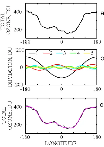
Fig. 1. The distribution of the TOMS total ozone values along
65◦S, 15 October 1996 (a), the spectral components of the wave numbers 1–5 (b) and comparison of the observed and the restored distributions (c).
location of the Ukrainian Antarctic station Akademik Ver-nadsky. The first results concerning the variations of plan-etary waves in total ozone at this latitude were obtained in Grytsai et al. (2005). For 1979–2003 the time interval of August-December covering the Antarctic late winter, spring and early summer was considered. The years of 1994 and 1995 are excluded because of the gaps in the satellite ozone data.
Expansion in series of the longitudinal distribution of the total ozone values f (λ) for the zonal wave number m is:
f (λ) =
∞
X
m=−∞
ameimλ, (1)
where λ is the longitude and the coefficient amis
am= 1 2π π Z −π f (λ) e−imλdλ. (2)
Figure 1 shows the example of the analysis made using Eqs. (1) and (2) to the TOMS distribution of the total ozone values at 65◦S. The standard deviation between the observed distribution (a) and restored one based on the wave numbers
1–5 (b) is 6.9 DU or 2.5% in this example and is typically 7–11 DU that can be attributed to the wave numbers higher than 5.
To describe the main properties of the zonal wave num-bers in each of the years quantitatively, the average ampli-tudes were calculated. First, the daily amplitude modules were averaged to obtain the amplitude Amgen, which charac-terizes the general wave event both in a stationary and trav-eling form: Am gen= 1 π N N X j =1 π Z −π fj(λ) e−imλdλ , (3)
where j is the day number, N is the total day quantity and
λis the longitude. The monthly and 5-month averages were obtained, which are presented in Sect. 4.
Then the amplitude Amst of the wave number stationary part was found by averaging the daily longitudinal profile
f (λ): Am st = 1 π N N X j =1 π Z −π fj(λ) e−imλdλ . (4)
The second procedure removes the anti-phase values of total ozone and accumulates in-phase ones, giving the amplitude
Amst and phase λst of the stationary wave component (see below in Sect. 5).
3 Zonal wave number 1–5 in 1996 and 2002
The variations of the daily zonal distributions of the total ozone in each of the wave numbers 1–5 during August-December were analyzed. The TOMS measurements for the southern winter at 65◦S are possible from late July; there-fore, August is the only winter month which is suited for the monthly data analysis. December was chosen as the last month of the indicated time interval, because the wave ac-tivity in total ozone, as it will be shown below, can be ob-served at the latitude 65◦S in early Antarctic summer. This agrees with the long-term tendency in the change in the polar stratospheric vortex duration. For example, during the last decades the date of the ozone hole disappearance, which is closely related to the breakdown of the polar vortex, shifted from November in the 1980s, to early December in the 1990s (Figs. 3–5 in WMO, 2003).
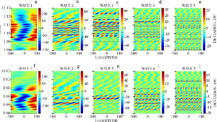
As examples, the years 1996 and 2002 are presented in Figs. 2a–e, and f–j, respectively. It is well known that during Antarctic spring 2002 the first recorded major stratospheric warming and splitting of the polar vortex in late September was observed (Baldwin et al., 2003). The vortex develop-ment in 2002 was very different from the preceding years and the vortex of 1996 was chosen as a typical event. At the latitude 65◦S the maximum speed of the zonal mean zonal wind in October 1996 exceeded 50 m/s at 20 hPa level (Hio and Yoden, 2004), whereas in late August and early Septem-ber 2002 the wind was ∼20–30 m/s weaker than normal and
abruptly weakened from 17 September (Allen et al., 2003; Baldwin et al., 2003; the data for 60◦S).
It is seen from Fig. 2 that the individual wave numbers show the highest activity during September-November, al-though a strong timing is not observed. Wave 1 exhibits a quasi-stationary behaviour, which is observed in 1996 up to early December (Fig. 2a). The latest interval of a wave ac-tivity one can see in the middle of December 1996 from the wave number 3 plot (Fig. 2c).
The eastward motion is seen as an increase in the east-ern longitude of the wave ridges and troughs in time, which becomes apparent in the slope of the color stripes in the time-longitude plots in Fig. 2. The intervals of relative phase sta-bility are sometimes observed. It is evident that each of the wave numbers can be observed in a standing form.
A time evolution of the spectral components in 2002 is very different (Figs. 2f–j; note the gap in the TOMS data during 2–12 August 2002). Figure 3 presents the distinc-tions between 1996 and 2002 as a change in periodicity of the traveling components. Figure 3 shows the result of wavelet-transform applied to the time-longitude distributions presented in Fig. 2. We have selected the 150-day time series of the wave number amplitude at the fixed longitude. The se-ries is an analogue of the single-point measurements which give the 5-month time variations of the individual wave num-ber.
As it is seen from Figs. 2b–e and g–j, the longitude can be selected arbitrarily for each of the wave numbers 2–5 be-cause of their regular zonal structure. Wave 1 has one lon-gitudinal cycle with a deviated phase of the stationary com-ponent. Since the time-longitude distribution in Figs. 2a,f gives the superposition of the traveling and quasi-stationary components of wave 1, a choice of longitude can correspond only to the intensity time change but not to the periodicity. We have selected the longitude of Vernadsky station 64◦W to analyze a periodicity in all of the wave numbers.
Figure 3 presents the changes in periodicity under condi-tions of a strong and weak polar vortex of 1996 and 2002, respectively, for the same spectral components as in Fig. 2. The range of periods is truncated at 20 days.
The main distinction between the two years is the presence of the quasi 7-day periods in wave 1–3 in 1996 (Figs. 3a-c), which is not observed in these wave numbers in 2002 (Figs. 3f–h). Note that the 7-day periods in the wave num-bers 1–3 during October 1996 have been considered by Hio and Yoden (2004) in more detail with respect to wave-wave interaction. Here we note the distinctive features in the char-acteristic periods of the spectral components.
In comparison to 1996, the wave numbers 1–3 in 2002 have the longer 8–12-day periods (Figs. 3f–h). The tendency of a systematic increase in the lower value of the wave 1 pe-riod is observed. The pepe-riod is changed from ∼7 days in August to 12–15 days in September and up to ∼20 days in early October.
The distinction in the wave 1–3 periods indicates different zonal phase velocity in 1996 and 2002. The shorter peri-ods in 1996 correspond to the higher zonal velocity, because
the wavelength is constant for each of the wave numbers at the fixed latitude circle. Similarly, the longer periods of the wave numbers 1–3 in 2002 characterize the lower phase ve-locity. In general, this agrees with the conditions of a strong and weak polar vortex, i.e. stronger and weaker zonal wind in 1996 and 2002, respectively. In the same way, an increase in the wave 1 period during August-September 2002 can be concerned with an intense deceleration of the zonal wind, which took place beginning in the second half of August (Baldwin et al., 2003).
A noticeable increase in the wave 1 period from 8 to 15 days during August-September (Fig. 3f) corresponds to the phase velocity decrease from 24 to 13 m/s (estimation was made for the length of wave 1 at the 65◦S latitude). The wave 2 and 3 velocities are equal to 8–9 and 5–6 m/s, respectively. The 7-day periods in 1996 give the higher phase velocities of 27, 14 and 9 m/s for waves 1–3, respectively.
The periods shorter than 7 days do not appear in waves 1–3 at all (Figs. 3a–c, f–h). But the periods in the range of 4–7 days exist in wave numbers 4–5, both in 1996 and 2002 (Figs. 3d–e and i–j, respectively). In the event of 2002 wave 5 shows the 7-day oscillation during October-November (Fig. 3j), whereas the polar vortex breakdown oc-curred in late September. Obviously, the wave 4–5 activity can exist independently of the polar vortex strength and du-ration. At least this situation is observed in the two events of 1996 and 2002.
It should be noted that the periods at the level of ∼5 days are absent in all analyzed years and the 7–20-day periods are predominant. As it is evident from spectral comparisons by Lawrence and Jarvis (2001) made for the Antarctic station Halley (76◦S, 26◦W) the 5-day periods in August are not observed and the 12–20 day periods are the most intense. This result is obtained for the 30-km level in the stratosphere for 1996.
More detailed quantitative analysis is necessary to deter-mine the interrelation between the individual wave number periodicity changes and polar vortex parameters. In this pa-per we focus further on the amplitude variations of the zonal wave numbers 1–5.
4 Variability of the amplitude of wave numbers 1–5
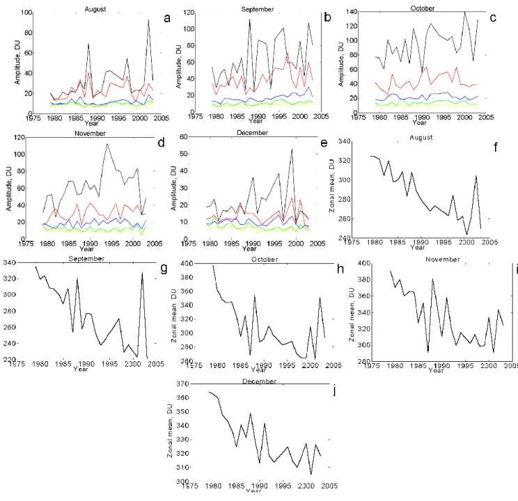
The interannual variations of the monthly mean amplitude of waves 1–5 during 1979–2003 are shown in Figs. 4a–e. Each of the months from August to December is presented on sep-arate plots. On the right the interannual variations of the total ozone zonal mean at 65◦S are presented for the same month sequence (Figs. 4f-j), to compare the relative contribution of waves 1–5 to the total ozone variability. Some individual features are peculiar to the development of wave 1–5 activity during each of months.
Wave number 1 has the largest amplitude and increasing trend in all of 5 months (Figs. 4a–e, black line). In August the largest anomalies in the wave 1 amplitude relative to the mean tendency are observed in 1988 and 2002 (wave
am-1568 A. Grytsai et al.: Planetary waves in total ozone
Fig. 2. Time-longitude variations of the daily deviation from the zonal mean at 65◦S for the wave numbers 1–5 during August-December 1996 (a-e) and 2002 (f-j).
Fig. 3. The periodicity variations of wave numbers 1–5 during August-December 1996 (a–e) and 2002 (f–j).
plitude of about 69 and 93 DU, respectively, see Fig. 4a). In September the wave 1 peak in 1988 (112 DU) is some-what higher than in 2002 (107 DU), and much higher relative to the mean tendency (about 60 and 30 DU, respectively). The quasi-biennial oscillations in the wave 1 amplitude are clearly seen in September. In October wave 1 has the largest amplitude with a peak value of 139 DU in 2000.
Wave number 2 shows some increasing trend in September only (Fig. 4b, red line). The change in amplitude from month
to month is relatively small in the range of 20–40 DU, except for December, with an average level of about 15 DU. Wave 2 is the closest to wave 1 in amplitude in August.
Wave number 3 has again a statistically significant in-crease of amplitude (at the 95% confidence level) in Septem-ber (Fig. 4b, blue line). During August-DecemSeptem-ber its ampli-tude varies at the level of 10–20 DU.
Wave numbers 4 and 5 with the amplitudes of about 5– 15 DU (Figs. 4a–e, green and yellow lines, respectively) have
Fig. 4. Interannual variations of the monthly mean amplitude of the wave numbers 1–5 for August-December (a–e) and zonal mean total
ozone at 65◦S (f–j) for the same months. Colors are black (wave 1), red (wave 2), blue (wave 3), green (wave 4) and yellow (wave 5).
a statistically significant level of 4–6% relative to the zonal mean during August-October in the late 1990s − early 2000s, when the zonal mean values are the lowest (240–280 DU, Figs. 4f–h). In early 1980s these wave numbers have a rel-ative amplitude of 2–3%, which is close to the noise level, when taking into account an error in the TOMS total ozone data of 1–2% (WMO, 1999).
A tendency in the interannual variations of the total ozone zonal mean at 65◦S should be noted separately. It is seen from Fig. 4 that the decreasing trend in August and Septem-ber is observed up to the early 2000s (Figs. 4f–g) and it ceases earlier and earlier: in the late 1990s in October
(Fig. 4h), and in early 1990s in November and December (Figs. 4i–j). Obviously, this is an indication of a global change in ozone dynamics. Similar tendencies, which allow one to predict the future ozone layer recovery, are widely re-ported and discussed in the last years (WMO, 2003; Fioletov, 2004; Randel, 2004).
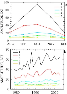
It is interesting to compare the distinctions in the ampli-tude trends for wave numbers 1–3. In Fig. 5 the results for the three months are presented, namely for August (red), September (blue) and October (black). Increasing trends in the wave 1 amplitude (Fig. 5a) are 11, 14 and 15 DU/decade in August, September and October, respectively.
1570 A. Grytsai et al.: Planetary waves in total ozone
Table 1. The values of the monthly mean amplitude of the wave numbers 1–5 and zonal mean total ozone at 65◦S (in Dobson Units), averaged for 1979–2003.
August September October November December
Wave 1 30.9 62.7 94.3 61.5 20.6 Wave 2 22.1 38.8 42.4 30.5 13.2 Wave 3 11.4 16.7 21.3 18.3 9.5 Wave 4 9.4 10.2 13.6 11.9 7.1 Wave 5 7.6 7.8 9.0 8.9 5.5 Zonal mean 286.9 275.2 310.2 334.8 331.9 Number of values 23 24 23 24 22
Fig. 5. Comparison of long-term trends in amplitude of the wave
numbers 1–3 during August (red line), September (blue line) and October (black line).
Statistically significant trends of about 8 and 5 DU/decade are observed in waves 2 and 3, respectively, in September only (Figs. 5b and c, blue line). So, a distinguishing feature of September is the clear tendency of an increasing long-term trend of waves 2–3 amplitude, which is not observed for these wave numbers in August and October.
Fig. 6. Monthly mean amplitude of the wave numbers 1–5 averaged
for the 1979–2003 period (a) and the interannual change of the 5-month mean amplitude (b).
In Fig. 6a, the monthly mean amplitudes 1–5 averaged through 1979–2003 are shown for each of the wave num-bers. These values are also summarized in Table 1. The nearly symmetric change in the wave 1 amplitude value rela-tive to the peak value of 94 DU in October is seen. This value is three times more than amplitude value in August. Note that wave 1 has almost an equal amplitude in September and November. Even in December the wave 1 activity exists at the mean amplitude level of 20 DU. Higher wave numbers do not exhibit the sharp change in the monthly means from month to month.
Another summarizing result is given in Fig. 6b, where the long-term change in the 5-month mean amplitude during
1979–2003 is shown. The most evident increase in the 5-month mean amplitudes is observed for the wave numbers 1 and 2, but this tendency is not kept in the last years. The am-plitudes averaged over 1979–2003 are 53.6, 29.9, 15.5, 10.5, and 7.8 DU for the wave number sequence 1, 2, 3, 4 and 5, respectively.
October’s peak in the wave 1 amplitude (Fig. 6a) displays the nature of wave disturbance of total ozone in the vortex edge region. Deformation of the stratospheric polar vortex by the planetary wave 1 results in a meridional displacement of stratospheric air. Because the vortex edge prevents one from mixing the mid-latitude and polar air masses during Antarctic winter and spring (Lee at al., 2001), wave deformation results in a displacement of the midlatitudinal ozone rich air, which accumulates outside the polar vortex, toward the pole and low ozone polar air toward the equator. In particular, this process is seen well visually from the time sequences of the TOMS total ozone fields (TOMS, 2004b).
An effect of such meridional air displacements in the op-posite directions is that the low and high ozone air which originated from different latitudinal bands appears at the lati-tude circle of 65◦S. This forms the waved distribution of total ozone along the circle of 65◦S, which displays the charac-ter and degree of vortex edge deformation: the more merid-ional displacement in wave structure, the more contrast in total ozone at the fixed latitude circle in this region. To-tal wave numbers contribute to a deformation of the vortex edge, but wave 1 is predominant. As it was shown in Grytsai et al. (2005), the long-term negative trends in the values of the quasi-stationary minimum and maximum in total ozone at 65◦S (by zonal distribution of the total wave numbers) are in agreement with the mean total ozone trends observed in the adjusted latitude bands.
The lowest total ozone and largest negative trend over Antarctica that are observed in October (WMO, 2003) can explain October’s maximum of the wave 1 amplitude (Fig. 6a, and Table 1), as well as its highest increasing trends indicated above. The vortex edge deformation and air dis-placement across the latitudinal circle, which arises from the zonal wave numbers 2 and 3, has the relatively smaller spa-tial scale. The stratospheric air mass, which forms the zonal distribution of the total ozone by waves 2 and 3, is limited by the narrower latitudinal band in the vortex edge region. Then the meridional difference in the mean ozone loss and negative trend is smaller than in the wave 1 case. It is possi-ble that this circumstance has an effect in the relatively lower amplitude and trend for waves 2–3 (Figs. 4a–e). The largest trend in the amplitude for waves 2–3 is observed in Septem-ber (Figs. 5b–c), which can be concerned with a minimum value of the zonal mean at 65◦S just in September (see Ta-ble 1).
Then the long-term change in the wave number ampli-tude in the southern vortex edge region is substantially deter-mined by the ozone loss in the polar stratosphere and increas-ing contrast between the total ozone at the polar and equa-torial side of the vortex edge. The quasi-columnar merid-ional displacement of air in the lower stratosphere (Salby and
Callaghan, 1993), caused by the planetary wave deformation of the polar vortex, obviously gives a main contribution to the observed variations of the zonal wave number amplitude.
5 Stationary component
From the averaging procedure Eq. (4) the 5-month mean lon-gitudinal distributions of total ozone are obtained. Figure 7 shows 23 curves (1979–2003) for each of the wave numbers 1–5 in order to present a degree of the interannual variabil-ity of the stationary component amplitude Amst and phase
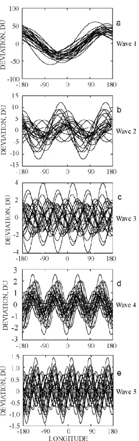
λst. It is shown that wave number 1 is inherent in the most stable longitudinal distribution of the total ozone (Fig. 7a). The wave numbers 2 and 4 also show some indications of the long-term phase stability (Figs. 7b and d). The stationary components of the wave numbers 3 and 5 are very change-able in amplitude and phase from year to year (Figs. 7c and e), but wave 4 exhibits enough stable longitudinal distribu-tion, although at the low amplitude level. The interannual variations of the 5-month average amplitude Amst are pre-sented separately in Fig. 8.
Finally, the average amplitude Amst and Amgen for the 1979–2003 period can be compared (Fig. 9). Each of the wave numbers 1–5 shows the presence of the stationary com-ponent, and it is predominant in the wave 1 behavior. For the waves 2 to 5 the traveling form is predominant. The 23-year average zonal distribution gives the amplitude sequence of 38.3, 4.8, 1.8, 1.2 and 0.7 DU for the stationary components of the wave numbers 1 to 5, respectively.
It is seen that the wave 2 contribution to the long-term sta-tionary distribution of total ozone is eight times less than the contribution of wave 1. This is close to the value of ∼1:6 ob-tained for the Southern Hemisphere October from the TOMS data of 1979–1986 in Wirth (1993).
The amplitudes Amst of waves 2–5 at the level of 1–5 DU do not noticeably influence the stationary ozone distribution on the many years scale, although they can increase tem-porarily on the monthly or weekly scale.
6 Conclusion
Planetary waves in the total ozone at the southern latitude of 65◦S have been analyzed in this work. The TOMS data spectral analysis was made to study the behaviour of zonal wave numbers 1-5 during August-December of 1979–2003. The first task was to establish whether the wave number pe-riodicity plays a part in the stratospheric polar vortex devel-opment. The activity of wave numbers 1–5 was considered under the conditions of the strong (1996) and weak (2002) vortex. The first three spectral components exhibit a distinc-tion in periodicity, with the lowest period of about 7 days in 1996, which is absent in 2002. Under conditions of the vor-tex 2002 the periods of 8–12 days predominate. The presence of a shorter period in 1996 in comparison with 2002 probably corresponds to the distinction in the zonal wind velocity, i.e. to the typically higher (lower) velocity in the strong (weak)
1572 A. Grytsai et al.: Planetary waves in total ozone
Fig. 7. Interannual changes of the stationary component of the wave
numbers 1–5 (a–e). The August-December averaging of the daily deviation from the zonal mean at 65◦S was used. The period of 1979–2003 is presented.
Fig. 8. Interannual variations of the stationary component
ampli-tude Amst of the wave numbers 1–5 (the colors are the same as in Fig. 6).
Fig. 9. Relationship between the wave number amplitude Amst (sta-tionary) and Amgen(general), averaged for the 1979–2003 period.
vortex. A noticeable increase in the wave 1 period from 8 to 15 days during August-September (Fig. 3f) can also indicate a deceleration of the zonal wind in the second half of August (Baldwin et al., 2003). The two last spectral components are observed in the range of periods 5–20 days, both in 1996 and 2002, i.e. regardless of vortex strength.
The second task of this work was to describe the monthly and interannual variations of the amplitude of zonal wave numbers 1–5. On a monthly scale the spectral components’ behaviour has individual features:
1. During August-December wave 1 has the largest ampli-tude (up to 139 DU in October 2000) and an increasing trend (up to 15 DU/decade for October 1979–2003); 2. The largest anomalies in the wave 1 amplitude relative
to the mean tendency is observed in 1988 and 2002 in August (Fig. 4a);
3. The quasi-biennial oscillations in wave 1 amplitude are clearly seen in September only (Fig. 4b);
4. In waves 2 and 3 the statistically significant trends of about 8 and 5 DU/decade, respectively, are observed in September only (Figs. 5b and c);
5. Wave numbers 4 and 5 show the monthly mean ampli-tudes of about 5–15 DU, which can be estimated as sta-tistically significant (4–6% relative to the zonal mean) during August-October in the late 1990s–early 2000s; in other time intervals they are close to the noise level due to the higher level of zonal mean total ozone at 65◦S; 6. The monthly mean amplitudes of wave 1 in
August-December, averaged on the 25-year time scale, is nearly symmetric relative to the peak value of 94 DU in Octo-ber. In December the wave 1 activity exists at the am-plitude level of 20 DU. The higher wave numbers do not show the sharp change in the monthly means from month to month.
The long-term change in the 5-month mean amplitude shows the most evident increase in amplitude for the wave numbers 1 and 2, but this tendency is not kept in the last years. The 5-month mean amplitudes averaged over 1979– 2003 are 53.6, 29.9, 15.5, 10.5, and 7.8 DU for the wave number sequence 1, 2, 3, 4 and 5, respectively. For the sta-tionary components the amplitudes are 38.3, 4.8, 1.8, 1.2, 0.7 DU, respectively. Thus, the wave 1 stationary component and the traveling component of waves 2–5 are predominant. The tendencies for a long-term change in the wave number amplitude can be explained by taking into account the degree of wave deformation of the polar vortex edge, net meridional displacements of the lower stratosphere air, and the contrast between total ozone on each side of the vortex edge (i.e. in polar and middle latitudes), which is determined by the dif-ference in the ozone loss and negative trends in these regions. Acknowledgements. We thank two anonymous reviewers for their constructive comments and helpful suggestions. This work was partly supported by grants FFD F7/362-2001 and STCU Gr-50(J).
Topical Editor U.-P. Hoppe thanks two referees for their help in evaluating this paper.
References
Allen, D. R., Bevilacqua, R. M., Nedoluha, G. E., Randall, C. E., and Manney, G. L.: Unusual stratospheric transport and mixing during the 2002 Antarctic winter, Geophys. Res. Lett., 30, 1599, doi:10.1029/2003GL017117, 2003.
Baldwin, M., Hirooka, T., O’Neill, A., and Yoden, S.: Major strato-spheric warming in the Southern Hemisphere in 2002: dynamical aspects of the ozone hole split, SPARC Newsletter, 20, 24–26, 2003.
Fioletov, V. E.: Total ozone variations over midlatitudes and on the global scale, OZONE, Volume I, XX Quadrennial Ozone Sym-posium, Proceedings, 25–26, 2004.
Fishbein, E. F., Elson, L. S., Froidevaux, L., Manney, G. L., Read, W. G., Waters, J. W., and Zurek, R. W.: MLS observations of stratospheric waves in temperature and O3 during 1992 Southern winter, Geophys Res. Lett., 20, 1255–1258, 1993.
Grytsai, A. V., Evtushevsky, A. M., and Milinevsky, G. P.: Interan-nual variations of planetary waves in ozone layer at 65◦S, Int. J. Rem. Sens., issue on XX Quadrennial Ozone Symposium, in press, 2005.
Hio, Y. and Hirota, I.: Interannual variations of planetary waves in the Southern Hemisphere stratosphere, J. Met. Soc. Jap., 80(4B), 1013–1027, 2002.
Hio, Y. and Yoden, S.: Quasi-periodic variations of the polar vor-tex in the Southern Hemisphere due to wave-wave interaction, J. Atmos. Sci., 61, 2510–2527, 2004.
Lawrence, A. R. and Jarvis, M. J.: Initial comparisons of plane-tary waves in the stratosphere, mesosphere and ionosphere over Antarctica, Geophys. Res. Lett., 28, 203–206, 2001.
Lee, A. M., Roscoe, H. K., Jones, A. E., Haynes, P. H., Shuck-burgh, E. F., Morrey, M. W., and Pumphrey, H. C.: The impact of the mixing properties within the Antarctic stratospheric vortex on ozone loss in spring, J. Geophys. Res., 106(D3), 3203–3211, 2001.
Randel, W. J.: Challenges for understanding global ozone vari-ability, OZONE, Volume I, XX Quadrennial Ozone Symposium, Proceedings, 17–18, 2004.
Salby, M. L.: Fundamentals of Atmospheric Physics, (Eds.) Dmowska, R. and Holton, R., Academic Press, 627, 1996. Salby, M. L. and Callaghan, P. F.: Fluctuations of total ozone and
their relationship to stratospheric air motions, J. Geophys. Res., 98(D2), 2715–2727, 1993.
TOMS ozone data, http://toms.gsfc.nasa.gov/ftpdata.html, 2004. TOMS ozone image, http://toms.gsfc.nasa.gov/ftpimage.html,
2004b.
Vargin, P. N.: Analysis of an eastward-propagating planetary waves from satellite data on the total ozone content, Izv. RAS. Phy. Atm. Ocean, (in Russian), 39, 327–334, 2003.
Wirth, V.: Quasi-stationary planetary waves in total ozone and their correlation with lower stratospheric temperature, J. Geophys. Res., 98(D5), 8873–8882, 1993.
WMO: Scientific Assessment of Ozone Depletion: 1998, World Meteorological Organization, Report No. 44, 1999.
WMO: Scientific Assessment of Ozone Depletion: 2002, World Meteorological Organization, Report No. 47, 2003.