Comparing the Homogeneity of Income Distributions using Polarization Indices

Cahier de recherche/Working Paper 15-12

Comparing the Homogeneity

of Income Distributions using

Polarization Indices

André-Marie Taptué

Abstract:

In the context of polarized societies, income homogeneity is linked to the frequency and

the intensity of social unrest. Most homogenous countries exhibit a lower frequency of

intense social conflicts and less homogeneous countries show a higher frequency of

moderate social conflicts. This paper develops a methodology to compare the degree of

homogeneity of two income distributions. We use for that purpose and index of

polarization that does not account for alienation. This index is the identification

component of polarization that measures the degree to which individuals feel alike in an

income distribution. This development leads to identification dominance curves and

derives first-order and higher-order stochastic dominance conditions. First-order

stochastic dominance is performed through identification dominance curves drawn on a

support of identification thresholds. These curves are used to determine whether

identification, homogeneity, or similarity of individuals is greater in one distribution than

in another for general classes of polarization indices and ranges of possible identification

thresholds. We also derive the asymptotic sampling distribution of identification

dominance curves and test dominance between two distributions using Intersection

Union tests and bootstrapped p-values. Our methodology is illustrated by comparing

pairs of distributions of eleven countries drawn from the Luxembourg Income Study

database.

Keywords: Alienation, Identification, Polarization, Stochastic dominance

1

Introduction

Income polarization is a consequence of an interaction between identification and alienation in an income distribution. Alienation measures dissimilarity between individuals with different incomes and identification measures the degree to which people belonging to the same group feel alike and identified to each other. An interaction between alienation and identification creates antagonism between groups and can lead to social unrest and civil war (Esteban and Ray,1994). However, putting a part discrepancies between incomes, social unrest is frequent in heterogeneous countries where people feel less alike and less identified to each other and it is rare in homogeneous countries where inhabitants feel more similar to each other in terms of income and even in terms of social characteristics. Therefore, choosing an income distribution that bears more homogeneity and identification within inhabitants can reduce the risk of conflict in a society.

Polarization studies measure identification with group sizes and assume that a distribution com-posed of many groups with small sizes is less homogeneous than a distribution comcom-posed of few groups with large sizes, which is said to be more homogenous (Esteban and Ray,1994). In the former distribu-tion, the frequency of social unrest is high though of a moderate intensity, and individuals feel less alike and less identified to each other than in the latter distribution that witnesses a lower frequency of social unrest though intense when it occurs (Esteban and Ray,2008). The best situation is when all individuals are encompassed in one income group. Hence, identification as measured in polarization can reveal not only the degree of similarity of individuals, but also the homogeneity of a distribution and the risk of social conflict.

This paper focuses on the identification component in a polarization index to order distributions by neglecting the interaction between identification and alienation. Integrating this procedure in a polariza-tion index leads to a reduced form of the index that measures the equality-like component of polarizapolariza-tion or the within-group homogeneity of a distribution. The equality and the homogeneity of a distribution correspond to the presence of many similar individuals with the same characteristics of interest such as income. Using the reduced form of a polarization index to compare homogeneity of two income distributions means to compare the importance of group densities in the two distributions.

Our methodology implements stochastic dominance technics to allow for robust comparisons of homogeneity between two distributions. With stochastic dominance, we go across a range of identifi-cation thresholds that represent densities that must not be exceeded by a density of any income group and derive an identification dominance curve. First-order stochastic dominance may hold until a cer-tain identification threshold lower than some acceptable values. The analysis can then be extended to second-order stochastic dominance and then to higher orders. On the whole, the exercise is performed continuously and it stops either when a maximum threshold of identification is reached or when the order

of the dominance is judged sufficiently high. A distribution has larger identification, is more homogenous or its individuals feel more alike if its dominance curve is always above that of a second distribution.

We also develop statistical inference tests and infer stochastic dominance from data samples for robust conclusions. We derive the sampling distribution of an estimator of the stochastic dominance curves and we perform statistical inference using bootstrapped p-values.

We begin inSection 2by showing how identification is measured in polarization indices.Section 3develops first-order, second-order and higher-order stochastic dominance, and characterizes the classes of polarization indices compatible with each order of dominance. An identification dominance curve is developed in the particular case of income distributions in Section 4. Section 5provides statistical inference by deriving the asymptotic properties of an estimator of dominance curves and implement-ing statistical tests. Section 6 compares income distributions of 11 countries using 2004 data from the Luxembourg Income Study database andSection 7concludes.

2

Identification in polarization measures

This section reviews some polarization indices in order to see how identification has been taken into account. In the framework of alienation and identification,Esteban and Ray(1994) suppose a popu-lation grouped into significantly-sized clusters such that members of each cluster are similar in terms of an attribute. The following citation shows the importance of group sizes and homogeneity in a distribu-tion :

" As the struggle proceeds, ’the whole society breaks up more and more into two hostile camps,

two great, directly antagonistic classes: bourgeoisie and proletariat.’ The classes polarize, so that they become internally more homogeneous and more and more sharply distinguished from one another in wealth and power " (Esteban and Ray(1994), p. 820).

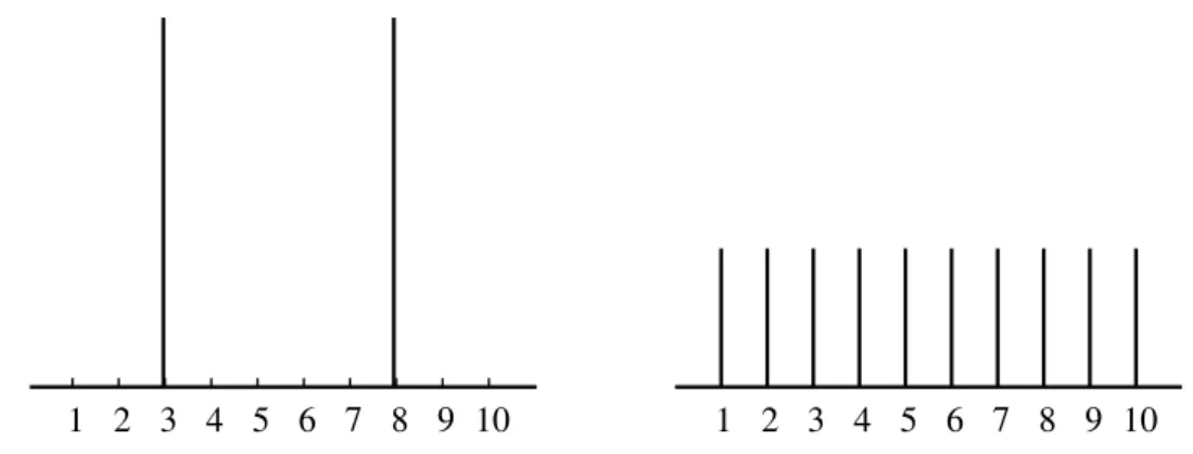
This view of homogeneity is supported byFigure 1first built byEsteban and Ray(1994) to illus-trate that there can be a high degree of within-group homogeneity in a polarized society. It shows that, departing from a society divided into two large groups relative to an attribute, group identification and consequently polarization can be reduced by clustering individuals in ten groups instead of two without caring about distances between them.

InFigure 1, the sizes of groups have decreased as well as polarization, while no attention has been paid to distances between groups during the process. For instance, consider two individuals respectively in groups 3 and 8 on the graph on the left, and suppose they are displaced respectively to groups 1 and 10 on the graph on the right. The distance between the two individuals has augmented from 5 to 9, but they are now in groups of smaller sizes and polarization has decreased. However, the risk of the emergence of

social conflict with a lower intensity is higher in the situation with 10 groups (Esteban and Ray,2008).

Figure 1: Reducing group sizes also reduces identification: A society composed of few groups of large sizes has more identification than a society composed of many groups of small sizes.

- - -

-1 2 3 4 5 6 7 8 9 -10 1 2 3 4 5 6 7 8 9 10

Duclos et al.(2004) use the traditional framework of alienation/identification for the measurement of polarization in the case where the distribution of the attribute of interest is described by a continuous density function. They propose the following formulation of the polarization index as the sum of all effective antagonisms in a society with a focus on income distributions:

P =

∫∫

p(a(x, y),ι(x)) f (x) f (y)dxdy (1) where p is the antagonism function, a(x, y) is the alienation function between the groups with income

x and y, ι(x) is the identification in the group with income x and f (.) is the income density. Then,

identification in a group can be measured as the density of income in that group (Duclos et al.(2004), p. 1740):

ι(x) = f (x) (2)

In a situation of pure income polarization where individuals identify themselves only with those with similar income, group sizes are estimated non-parametrically using kernel procedures.

3

Stochastic dominance

3.1 First-order stochastic dominance

Let PAbe a polarization index in a population A as defined inDuclos et al.(2004) and written here

in its general form:

PA = ∫∫ p(a, i)dF(a, i) (3) = ∫ _∞ 0 ∫ _∞ 0

p(a, i) f (a, i)dadi (4) where p(., .) is the antagonism function taking alienation and identification as arguments, F(., .) is the joint cumulative distribution function of alienation and identification and f (., .) the corresponding joint density. Alienation and identification are two variables defined inR+.

When alienation is negligible in a society, the antagonism function no longer depends on it so that

p(a, i)∝ p(i) and we can set

PA =

∫ _∞ 0

p(i) f (i)di (5)

where f (i) is the density of identification. For a decomposition of PA, we integrate it proceeding first to

a substitution: ι = −i. Then,

PA =

∫ 0

−∞p(−ι) f (−ι)dι (6)

Next, integrating PAby parts yields

PA = p(−ι) ∫ _ι −∞f (−i)di| ι=0 ι=−∞+ ∫ 0 −∞p 1_(−ι) (∫ _ι −∞f (−i)di ) dι (7) = p(0) ∫ ₀ −∞f (−i)di + ∫ ₀ −∞p 1_(−ι) (∫ _ι −∞f (−i)di ) dι (8) = p(0) ∫ _∞ 0 f (i)di + ∫ _∞ 0 p 1_(ι) (∫ _∞ ι f (i)di ) dι (9)

where p1is the first-order derivative of the antagonism function with respect to identification. Let z_ι≥ 0 be an identification threshold and let HA(zι) =

∫_∞

z_ι fA(i)di denote the identification

dom-inance curve function in a population A. HA(zι) is the proportion of individuals for whom identification

in their groups is greater than z_ι. We have∫₀∞f (i)di = HA(0) = 1 and

PA = p(0) +

∫ _∞ 0

The identification dominance curve function H(z_ι) is defined analogously for a distribution B:

PB = p(0) +

∫ _∞ 0

p1(ι)HB(ι)dι. (11)

Let E1denote the class of polarization indices in the form ofEquation (5)where the antagonism function is increasing in identification.

E1={P in the form ofEquation (5)| p1≥ 0}. (12) We are searching conditions under which distribution A is more homogenous (always has more identi-fication) than distribution B regardless of the polarization index in E1, that is, conditions under which

PA− PB≥ 0 for all P ∈ E1:

PA− PB=

∫ _∞ 0

p1(ι)(HA(ι) − HB(ι))dι. (13)

Consider P ∈ E1 and suppose that HA(zι)− HB(zι)≥ 0 whatever the identification threshold zι≥ 0.

Since p1≥ 0, ∆P = PA− PB ≥ 0 as an integral of a positive function in a closed interval. That is, the

condition HA(zι)− HB(zι)≥ 0 for all zι≥ 0 is a sufficient condition to compare distributions A and B

with polarization indices in E1.

For the necessity condition, suppose that PA− PB≥ 0 for all P ∈ E1 and that on the other side,

HA(zι)− HB(zι) < 0 for zι∈ [zι, zι+ε] for a small value of ε > 0. We define an antagonism function by:

p(ι) =          z_ι ifι ≤ z_ι ι if zι<ι ≤ zι+ε z_ι+ε if ι > z_ι+ε

The first-order derivative of the antagonism function with respect to identification is p1(ι) =∂p(ι)_∂ι = 1 in [z_ι, z_ι+ε], and 0 elsewhere. So, equationEquation (13)becomes:

PA− PB=

∫ z_ι+ε

z_ι

(HA(ι) − HB(ι))dι. (14)

With the hypothesis that HA(zι)−HB(zι) < 0 in [zι, zι+ε], we also have

∫_zι+ε

zι (HA(ι) − HB(ι))dι < 0 which implies that PA−PB< 0 and contradicts the assumption of PA−PB≥ 0. The necessary condition

is then verified.

Distribution B is therefore said to stochastically dominate distribution A at first order in the iden-tification component of polarization if HA(zι)− HB(zι)≥ 0 for all zι≥ 0. When the above condition is

fulfilled, there are always more groups with densities greater than any identification threshold in distri-bution A than in distridistri-bution B, and the identification dominance curve of A is always above that of B.

As a result, income groups in distribution A have more similar individuals and are more homogenous than income groups in distribution B. We note B≽ A to mean that B is less homogenous than A and stochastically dominates A at first order.

Proposition 3.1 . E1identification dominance at first order: Given two distributions from two distinct populations A and B,

B≽ A for all P ∈ E1iff HA(zι)− HB(zι)≥ 0 for all zι≥ 0.

3.2 Second-order stochastic dominance

A distribution B is less homogenous and stochastically dominates another distribution A at first order if the identification dominance curve of B, HB(zι), always lies below the identification dominance

curve of A, HA(zι), across a range of identification thresholds zι. However, instead of having dominance

in the entire interval of identification thresholds, distribution B might stochastically dominate distribution

A at first order only from a certain value of identification threshold z1_ι.

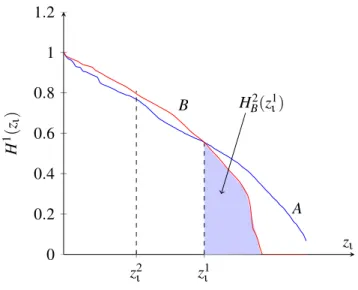
Two situations can occur when distribution B stochastically dominates distribution A: Either dom-inance holds in the entire interval of identification thresholds, or else domdom-inance reverses at the value

z1_ι where the two identification dominance curves intersect (Figure 2). The first case corresponds to the dominance in the sense ofFoster and Shorrocks(1988) while the second case implies the definition of z1_ι as

z1_ι = sup{z_ι> 0|HA(zι) < HB(zι)}. (15)

The situation where z1

ι > 0 opens a possibility for second-order stochastic dominance. To see how,

consider the expression of the polarization index fromEquation (10):

PA = p(0) +

∫ _∞ 0

p1(i)HA(i)di. (16)

Settingι = −i yields:

PA = p(0) +

∫ 0

−∞p

1_(−ι)H

A(−ι)dι. (17)

Then, integrating by parts leads to:

PA = p(0) + p1(ι) ∫ _ι −∞HA(−i)di| 0 −∞+ ∫ 0 −∞p 2_(−ι) (_{∫ ι} −∞HA(−i)di ) dι (18) = p(0) + p1(0) ∫ 0 −∞HA(−i)di + ∫ 0 −∞p 2_(−ι) (∫ _ι −∞HA(−i)di ) dι (19) = p(0) + p1(0) ∫ _∞ 0 HA(i)di + ∫ _∞ 0 p2(ι) (∫ _∞ ι HA(i)di ) dι (20)

where p2is the second-order derivative of the antagonism function with respect to identification. Let H2(ι) =∫_ι∞H(i)di be defined on the support of identification. Since H2(0) = 1, the above development of the polarization index becomes:

PA = p(0) + p1(0)HA2(0) + ∫ _∞ 0 p2(ι)H_A2(ι)dι = p(0) + p1(0) + ∫ _∞ 0 p2(ι)H_A2(ι)dι. (21) The analogous quantity can be written for a distribution B:

PB = p(0) + p1(0) + ∫ _∞ 0 p2(ι)H_B2(ι)dι. Thus,∆P = ∫ _∞ 0 p2(ι)(H_A2(ι) − H_B2(ι))dι. (22) Let E2denote the class of polarization indices in the form ofEquation (5)where the antagonism function is convex in identification.

E2={P in the form ofEquation (5)| p2≥ 0}. (23) We are searching conditions under which∆P = PA− PB≥ 0 for all P ∈ E2. Consider P ∈ E2and

suppose that H_A2(z_ι)− H_B2(z_ι)≥ 0 regardless of the identification threshold z_ι≥ 0. Since p2≥ 0, ∆P ≥ 0 for the same reasons as above. That is, the condition H_A2(z_ι)− H_B2(z_ι)≥ 0 for all z_ι≥ 0 is a sufficient condition for second-order stochastic dominance.

For the necessity condition, suppose that PA−PB≥ 0 for all P ∈ E2and that H_A2(zι)−HB2(zι) < 0 for

z_ι∈ [z_ι, z_ι+ε] for a small value of ε > 0. We define an antagonism function by: p(ι) =          z2_ι ifι ≤ z_ι ι2 _{if z} ι<ι ≤ zι+ε (z_ι+ε)2 _{ifι > z} ι+ε

The second-order derivative of the antagonism function with respect to identification is p2(ι) = 2 in [z_ι, z_ι+ε], and 0 elsewhere. So, equationEquation (22)becomes:

PA− PB=

∫ zι+ε

zι

2(H_A2(ι) − H_B2(ι))dι. (24) With the hypothesis that H_A2(z_ι)− H_B2(z_ι) < 0 in [z_ι, z_ι+ε], we have∫_zz_ιι+ε(H_A2(ι) − H_B2(ι))dι < 0 which

implies that PA− PB< 0 and contradicts the assumption of PA− PB≥ 0. The necessary condition is then

verified. We note B≽2A to mean that B stochastically dominates A at second order.

Proposition 3.2 . E2 identification dominance at second order: Given two distributions from two dis-tinct populations A and B,

As in first-order stochastic dominance, two situations can occur: either B stochastically dominates A at second order everywhere, or else there exits z2_ι ( seeFigure 2) defined by

z2_ι = sup{z_ι> 0|H_A2(z_ι) < H_B2(z_ι)} (25) from which B stochastically dominates A at second order. This suggests to check for dominance at order three.

Figure 2: Identification dominance curves for two distributions A and B

0 0.2 0.4 0.6 0.8 1 1.2 z1_ι z2_ι B A z_ι H_B2(z1_ι) H 1 (z ι )

3.3 Higher-order stochastic dominance

The above procedure can be developed for stochastic dominance at order s > 2. The polarization index integrated by part s times with respect to identification leads to :

P = p(0) + p1(0) +··· + ps−1(0)

∫ _∞ 0

ps(ι)Hs(ι)dι.

where ps is the sth-order derivative of the antagonism function with respect to identification, Hs(ι) =

∫_∞

ι Hs−1(i)di for s≥ 2 and H1(ι) = H(ι).

For two populations A and B,

∆P = ∫ ∞

0

ps(ι)(H_As(ι) − H_Bs(ι))dι. (26) Let Esdenote the sub class of polarization indices in the form ofEquation (5)defined as:

Suppose that H_As(z_ι)−H_Bs(z_ι)≥ 0 for all z_ι≥ 0, then ∆P ≥ 0 which fulfills the sufficient condition. For the necessity condition, assume PA− PB ≥ 0 and consider the following function of antagonism.

p(ι) =          zs_ι ifι ≤ z_ι ιs _{if z} ι<ι ≤ zι+ε (z_ι+ε)s _{ifι > z} ι+ε

Its sth-order derivative with respect to identification is ps(ι) = s! in [z_ι, z_ι+ε], and 0 elsewhere. Then: PA− PB= ∫ z_ι+ε zι s! (H_As(ι) − H_Bs(ι))dι. (28) Suppose H_As(z_ι)− Hs B(zι) < 0, then ∫_zι+ε

z_ι (HAs(ι) − HBs(ι))dι < 0, which implies that PA− PB< 0 and

contradicts the assumption of PA− PB≥ 0. The necessary condition is then verified. We note B ≽sA to

mean that B stochastically dominates A at sthorder.

Proposition 3.3 . Es identification dominance at order s: Given two distributions from two distinct populations A and B,

B≽sA for all P ∈ Esiff H_As(zι)− HBs(zι)≥ 0 for all zι≥ 0.

For each dominance order s, let an identification limit zs_ιdefined by

zs_ι = sup{z_ι> 0|H_As(z_ι) < H_Bs(z_ι)}. (29) The procedure stops either when the value zs_ι is judged to be sufficiently high or when we reach the maximum value of z_ι. In the first case, zs_ι has become greater that a reasonable maximum value of identification threshold. In the second case, stochastic dominance is achieved everywhere.

4

Case of income distributions

In this section, the identification dominance curve H(z_ι) is explained in the space of income where identification is measured with a density of income:

ι(y) = f (y). (30) H(z_ι) becomes: H(z_ι) = ∫ _∞ zι dFf(χ) (31) = 1− Ff(zι) (32)

where Ff is the cumulative distribution function of income densities and H(zι) is the hatched area of

Figure 3: Identification dominance curve for z_ι, H(z_ι): Proportion of individuals whose income density (identification) is greater than z_ι

Density of densities curve

Income density: f(y)

Density of densities f(f(y)) HA(zι) z_ι

5

Estimation and inference

This section is devoted to statistical inference of dominance relations between two identification dominance curves. It arrives that dominance observed in two distributions using dominance curves is induced by noise in samples. Furthermore, when two curves are close, we cannot conclude about the presence of dominance even if one is always above the other. We propose an estimator of H(z_ι) and we test dominance using an Intersection-Union [IU] test. The IU test introduced byBerger(1982) and used byBerger and Sinclair(1984) andBerger(1996) consists of choosing the null hypothesis as a union of simple hypotheses and the alternative hypothesis as an intersection of simple hypotheses.

5.1 Distribution and critical frontiers

Consider a random sample of N independently and identically distributed observations of income

y1,··· ,yN drawn from a distribution with a cumulative distribution function F. An estimator of H(zι) is

defined by : ˆ H(z_ι) = ∫ I( ˆf (y)≥ z_ι)d ˆFf(χ) (33) = N−1 N

∑

The income density f is estimated non parametrically with the Gaussian kernel function: ˆ f (yi) = N−1 h√2π N

∑

where h is the optimal bandwidth of Silverman, proposed to trade off reductions of bias and variance:

h = 1.06 ˆσN−15

where ˆσ is an estimator of the standard deviation of income, which is conditional on the gap between the first and the third quartile. Let Q(0.25), Q(0.75) andσ denote respectively the estimates of the first and the third quartiles, and the standard deviation of the distribution. Then,

ˆ σ =    Q(0.75)−Q(0.25) 1.34 if Q(0.75)−Q(0.25) 1.34 <σ σ if Q(0.75)_1.34−Q(0.25) ≥ σ. (34)

The existence of the population moment of order 1 allows us to apply the law of large numbers to

Equation (33)and deduce that ˆH(z_ι) is a consistent estimator of H(z_ι). The central limit theorem allows us to assert that this estimator is root-N consistent and asymptotically normal. Finally, the asymptotic distribution of the estimator of the identification dominance curve is defined inTheorem 5.1:

Theorem 5.1 N12( ˆH(z_ι)−H(z_ι)) is asymptotically normal with mean zero, and the structure of the

vari-ance is given by:

lim N→∞NVar( ˆH(zι)− H(zι)) = (1− Ff(zι))Ff(zι) + J −2

_∑

∑

[E(θj(zι)| f (y) ≥ zι)− E(θj(zι))] (35)

where there exist y∗₁,··· ,y∗_j,··· ,y∗_J| f (y∗_j) = z_ι,

θj(zι) = f (yˆ ∗j) ff , j(zι), (36) ff , j(zι) = N−1 N

∑

where kpand kf are Gaussian kernel functions defined respectively in the income and density spaces,

Var(θj(zι)) = ff , j2 (zι) N−1 h f (y ∗ j) ∫ k2_p(ψj)dψj whereψj= y−y∗_j h , (38)

E(θj(zι)| f (y) ≥ zι) = ff , j(zι)E( ˆf (y∗j)| f (y) ≥ zι), (39)

and E(θj(zι)) = ff , j(zι)

∫

kp(ψj) f (hψj+ y∗j)dψj. (40)

(Proofs are given in the appendix).

We also study the convergence in probability of the estimator ˆH(z_ι) through a Monte Carlo simu-lation. We first take an identification threshold z_ι= 0.00002. Next we draw three sets of 1000 samples from a log-normal distribution of mean zero and standard deviation 1 with sample sizes set respectively to 1000, 5000 and 10 000 observations. We draw the density of the estimators obtained from the 1000 simulated samples. InFigure 4, the density curves narrow in as the sample size increases. This tendency shows that the estimator ˆH(z_ι) is convergent. The distribution of the estimator is biased on the right when the sample size is 1000. We attribute this tendency to the fact the gaussian kernel estimator is higher and less concentrated in samples with small sizes. The gaussian kernel estimator is not efficient when the size of a sample is small.

Figure 4: Density curves showing the convergence of ˆH(z_ι) when z_ι= 0.00002. For each sample size N, 1000 samples are drawn from a log-normal distribution of mean zero and standard deviation 1

0 5 10 15 20 Density 0 .08 .16 .24 .32 .4 N=1000 N=5000 N=10000 ˆ H(0.00002)

The identification dominance curve H(z_ι) equals 1 when z_ι= 0 and 0 for large values of z_ι in any distribution. Thus, at the lower and upper bounds of identification thresholds, two identification dominance curves are confounded and dominance is expected in a restricted interval of identification

thresholds. The appropriate range of thresholds that can order distributions can be estimated. Consider two income distributions from two populations A and B where the interest is about the dominance of A by

B. For distribution B to dominate distribution A, there must exist a threshold z−_ι > 0 from which HA(zι)

begins to be greater than HB(zι):

z−_ι = sup{z_ι> 0|HA(zι) < HB(zι)}. (41)

From this lower critical frontier z−_ι , either HB(zι)≤ HA(zι) for all zι≥ z−_ι and distribution B stochastically

dominates distribution A everywhere above z−_ι , or else there exists a reversal identification threshold

z+_ι > z−_ι up to which dominance applies. The upper critical frontier z+_ι is the maximum identification threshold up to which distribution B stochastically dominates distribution A at first order. It is defined by:

z+_ι = sup{z_ι> z−_ι |HB(zι)≤ HA(zι)}. (42)

5.2 Testing dominance

Testing for dominance implies addressing two issues, that of the choice of the null and alternative hypotheses and that of the test statistic. Davidson and Duclos (2000) present three nested hypotheses that could be used either as the null or as the alternative hypothesis in dominance tests. The first one is

H0: HA(zι)− HB(zι) = 0 for all zι≤ z+_ι . The second one is H1: HA(zι)− HB(zι)≥ 0 for all zι≤ z+_ι and

the third and last one is H2without any restriction on HA(zι)− HB(zι). The three hypotheses are nested

in the sense that H0⊂ H1⊂ H2.

McFadden(1989) proposes to test H0 against H1 with the test statistic of the supremum. It is a

form of the Kolmogorov-Smirnov test used to test the identity of two distributions. The main difficulty in the test of McFadden is to tract the asymptotic properties of the test statistic under the null hypothesis. Also, it supposes that the two samples under consideration have the same sizes, which is not always the case.

The approach proposed byKaur et al.(1994) [KPS] seems more appropriate. The minimum value of test statistics at different alienation thresholds is used as the test statistic for the null of nondominance against the alternative of dominance. One advantage of this formulation is that if we reject the null hypothesis, all that remains is the alternative of dominance (Davidson and Duclos, 2013). This test is the Intersection-Union test and the probability of rejection of the null when it is true is shown to be asymptotically bounded by the nominal level of a test based on the standard normal distribution (Davidson and Duclos,2000).

So, we propose the following test of H₀ι against H₁ιto test the dominance of A by B:    H₀ι: HB(zι)≥ HA(zι) for some zι∈ [z−_ι , z+_ι ] H₁ι: HB(zι) < HA(zι) for all zι∈ [z−_ι , z+_ι ]. (43)

A procedure to perform this test consists of using a predetermined grid of points corresponding in our case to identification thresholds (Howes,1993). The only precaution is to be sure to cover entirely the interval of interest. The properties of the IU test using a grid of points are similar to those of the KPS test.

The null hypothesis is a union of simple hypotheses and the alternative hypothesis is an intersection of simple hypotheses. In this case, evidence against the null hypothesis exists when it also exists for every simple null hypothesis. If each simple test is of levelα, then the IU test is also of level α following theorems 1 and 2 ofBerger(1982). Furthermore,Berger and Sinclair(1984) show that not only the IU test is of levelα, but it is exactly of size α.

We suppose that the two distributions are independent. The KPS statistic is defined as the minimum over alienation thresholds of the simple test statistics. Consider the following simple test (of H₀zιagainst

H₁zι) for the dominance of A by B when the identification threshold is z_ι:    H₀zι: HB(za)− HA(zι)≥ 0 H₁zι: HB(zι)− HA(zι) < 0 (44)

The test statistic associated to this simple test is

tzι=

ˆ

HB(zι)− ˆHA(zι)

√

Var( ˆHA(zι))+Var( ˆHA(zι))

Because of the assumption on the independence of the two distributions, the variance of ˆHA(zι)−

ˆ

HB(zι) is the sum of their variances. Under the null hypothesis, there is no loss to take HA(zι) = HB(zι), a

condition under which tz_ιtends asymptotically to the standard normal distribution

N

level α, there is strong evidence against the null hypothesis of this simple test if the test statistic tzι is lower than the critical value of the standard normal distribution at the levelα. The test statistic of the IU test is defined by: t = min{tz_ι} for zιin the grid of thresholds . There is strong evidence against the null

hypothesis of the IU test at the nominal levelα if there is strong evidence against all simple tests. In that case, the test statistic t is lower than the critical value of the standard normal distribution at the levelα.

The evidence against the null hypothesis can be tested using p-values. A p-value is defined as a measure of the strength of the evidence against the null hypothesis and is determined as the probability of getting a value greater than or equal to the test statistic. We perform statistical test using a bootstrap approach because it gives better results than asymptotic tests, being more efficient. This choice avoids facing the problem of the bias in the estimator for samples of small sizes:

consider two income distributions A and B where we want to test the dominance of A by B, and a grid z1_ι, z2_ι,··· ,zk_ι,··· ,zM_ι of M points of identification thresholds. Here is the procedure to compute bootstrapped p-values.

1. consider an identification threshold zk_ι on the grid, say the first one;

2. draw a pair of samples with replacement from A and B of the same sizes as the initial samples and compute ˆd₁k= ˆHB(zk_ι)− ˆHA(zk_ι);

3. repeat the previous step (step 2) S independent times;

4. for each sample pair s = 1, 2,··· ,S, keep the estimate ˆd_sk= ˆHB(zk_ι)− ˆHA(zk_ι);

5. the p-value of the simple test with zk_ι is given by pk= S−1∑s=1S I( ˆdsk≥ 0) (Duclos and Araar,2006);

6. for the rest of identification thresholds zk_ι, k = 2,··· ,M, repeat steps 2 to 5.

The result is a pair (zk_ι, pk) of identification thresholds and corresponding p-values. The p-value

pkindicates the maximum probability that an error is made when we reject the null hypothesis in favour

of the alternative in the simple test with zk_ι. For a significance levelα, the null hypothesis of the simple test is rejected if pk≤ α.

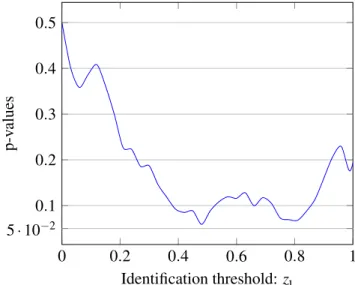
A decision on the IU test inEquation 43can be taken graphically by drawing the curve of p-values as a function of identification thresholds. Dominance exists where the p-value curve lies beneath the level of the test. For instance, considerFigure 5below of the dominance test between two hypothetical distributions A and B, on which we have p-values on the vertical axis and identification thresholds on the horizontal axis. For this illustrative example and for the traditional significance level of 5%, the null hypothesis is never rejected since p-values are always greater than 0.05 regardless of the threshold. However, the null hypothesis is sometimes rejected when the significance level is set to 10%. In this last case, the null hypothesis cannot be rejected until the threshold reaches 0.39. From this threshold, p-values remain less than 10% until the threshold is 0.51. The critical frontiers can then be fixed respectively to

Figure 5: Graphical illustration of a statistical test with p-value at different identification thresholds 0 0.2 0.4 0.6 0.8 1 0.1 0.2 0.3 0.4 0.5 5· 10−2 Identification threshold: z_ι p-v alues

6

Empirical illustration using LIS data

6.1 Data and statistics

We apply the above methodology to 2004 data of 11 countries from the Luxembourg Income Study (LIS) database (see Table 1). The LIS database contains harmonized microdata from countries which are exclusively middle and high-income countries. It also contains variables on household income, taxes and transfers, households and individual characteristics, labor market outcomes, and expenditures. We use disposable household income, defined as post tax and post transfer income of the household. The household income is adjusted through the division by an adult equivalent scale s0.5 where s is the household size. This operation is introduced to provide comparable incomes for individuals living in households of different sizes. We also weighted all household observations by the household weight "hweight normalized" multiplied by the number of people in the household unit. Some (less than 0.5%) incomes are negative in each country. We could have set these values to zero but we did not, assuming their impact is not significant on results. Income is also normalized by the mean to eliminate the problem of measurement units.

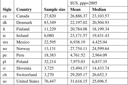
To compute some statistics like the mean and median incomes, national currencies are converted into US $ with 2005 purchasing power parities (PPP) from the 2005 International Comparison Program. Sample sizes for each country are shown in the first column ofTable 1. This table also summarizes the mean and the median of the adjusted household net income of each country set in US $. The USA has

the highest mean income ($31,616.15) among the 11 countries. It is followed by Switzerland with a mean of $29,205.55. The lowest mean income is that of Peru ($4,761.52). For countries like Mexico and Poland, the mean incomes are less than 10,000 dollars, but are greater than that of Peru. The Switzerland median income found to be $26,652 is the highest followed by the USA with a median income found to be $25,696.50. The lowest values of the median income are those of Peru ($2,964.09) and Mexico ($4,425.04).

Table 1: Sample sizes, mean and median income for 11 countries. Year=2004. $US, ppp=2005

Sigle Country Sample size Mean Median ca Canada 27,820 26,886.37 23,103.57 dk Denmark 83,349 22,197.02 20,504.93 fi Finland 11,229 20,784.08 18,199.34 ie Ireland 6,080 23,171.57 19,431.43 mx Mexico 22,595 6,938.19 4,425.04 no Norway 13,131 27,754.11 24,599.64 pe Peru 18,383 4,761.52 2,964.09 pl Poland 32,214 7,975.03 6,837.35 si Slovenia 3,725 15,494.17 14,433.74 ch Switzerland 3,270 29,205.17 26,652.3 us United States 76,447 31,616.15 25,696.5

The 2005 PPPscome from the 2005 International Comparison Program

6.2 Results

The application is limited to stochastic dominance at first order. The results are presented in two parts. The first part presents comparisons of pairs between the 11 countries based on identifica-tion dominance curves. A country whose identificaidentifica-tion dominance curve is always above another one regardless of the identification threshold has more identification and is more homogenous. A coun-try B stochastically dominates at first order another councoun-try A when there exist z−_ι and z+_ι for which

HB(zι)≤ HA(zι) for all zι∈ [z−_ι , z+_ι ]. Then income groups in B are less homogenous than income groups

in A, or individuals belonging to a same income group in A feel more alike than individuals belonging to a same income group in B.

Using identification dominance curves like those inFigure 7, we see that the USA stochastically dominates (is less homogeneous than) all the other countries except Mexico and Peru (Figure 6). Apart

from these two countries, HU SA(zι)≤ HCountry(zι) for any identification threshold zι. The proportion of

individuals whose income densities are greater than any identification threshold is lower in the USA than in the other countries. That is, people in Canada, Denmark, Finland, Ireland, Norway, Poland, Slovenia and Switzerland feel more alike and are more homogenous than people in the USA. As a result, income distributions in these countries are more homogenous than the income distribution in the USA. The results for pairwise comparisons are presented inTable 2.

For small values of identification thresholds, the USA is more homogeneous than Mexico and Peru, but the situation reverses for higher values of identification thresholds (Figure 6). Mexico stochastically dominates at first order the USA for z_ι∈]0,0.6] and Peru stochastically dominates at first order the USA for z_ι∈]0,0.77]. The identification dominance curves of the USA drawn across these intervals are always above those of Mexico and Peru, and outside these intervals, the identification dominance curves of the USA are always below those of the two countries.

Canada stochastically dominates everywhere at first order Denmark, Finland, Ireland, Norway, Slovenia and Switzerland. Then, the income distribution in Canada is less homogeneity than income distributions in these countries. As a consequence, the identification dominance curve of Canada is always below those of these countries. However, Canada is stochastically dominated by Mexico and Peru in restricted intervals. Mexico stochastically dominates (is less homogeneous than) Canada at first order for z_ι∈ [0,0.74]. So, in Canada, individuals whose income densities are lower than or equal to 0.74 feel more alike than the corresponding individuals in Mexico. Likewise Peru stochastically dominates Canada at firs order for z_ι∈ [0,0.85]. Further, Canada is as homogeneous as Poland.

Denmark is stochastically dominated at fist order by all the other countries, that it is more ho-mogeneous than the rest of the countries. Dominance of Denmark is achieved everywhere by Ireland, Mexico, Peru, Poland, Switzerland and the USA. Income distributions in these countries are less homo-geneous than the income distribution in Denmark. Then the income distribution in Denmark leads to groups of individuals who feel more alike compared to income distributions in Ireland, Mexico, Peru, Poland, Switzerland and the USA. Countries as Finland, Norway and Slovenia dominate Denmark in restricted intervals. Dominance is achieved in [0, 0.93] for Finland, [0, 0.92] for Norway and [0, 0.94] for Slovenia. For higher densities of income, Denmark appeared to be less homogeneous than the above countries. In fact, curves are confounded in the queues of distributions and the decision about dominance is ambiguous due to the small number of observations in the extreme of distributions.

The income distribution in Finland is as homogenous as the income distribution in Slovenia, mean-ing that individuals belongmean-ing to a same income group in Finland feel as alike as those from the same income group in Slovenia. Finland is stochastically dominated everywhere by Ireland, Mexico, Peru, Poland and Switzerland at first order, but Finland stochastically dominates Norway everywhere at first order. In Norway the income distribution is more homogenous than the income distribution in Finland

where the income in turn is more homogeneous than those of the other countries.

Ireland is less homogeneous than Norway and Slovenia, but it is more homogeneous than Mexico, Peru, Poland, Switzerland and the USA. In fact, Ireland stochastically dominates everywhere Norway and Slovenia, but it is stochastically dominated by Mexico, Peru, Poland, Switzerland and the USA. Dominance by Switzerland and the USA is achieved everywhere while dominance by Mexico, Peru and Poland is achieved in restricted intervals of identification thresholds. The identification thresholds up to which these last three countries dominate Ireland are found to be respectively 0.76, 0.79 0.72. Above these values, they are dominated by Ireland. Mexico is less homogeneous than Norway, Poland, Slovenia and Switzerland and is more homogeneous than Peru.

Norway is less homogeneous than Slovenia and is more homogeneous than Peru, Poland, Switzer-land and the USA. Peru is less homogeneous than PoSwitzer-land, Slovenia, SwitzerSwitzer-land and the USA, PoSwitzer-land is less homogeneous than Slovenia, Switzerland and the USA, and finally Slovenia is more homogeneous than Switzerland and the USA.

Table 2: Result of identification dominance between 11 countries based on their identification dominance curves ca dk fi ie mx no pe pl si ch dk ≼ fi ≼ r≽ ie ≼r ≽ ≽ mx r≽ ≽ ≽ r≽ no ≼ r≽ ≼ ≼ ≼ pe r≽ ≽ ≽ r≽ ≽ ≽ pl ≊ ≽ ≽ r≽ ≼ ≽ ≼ si ≼ r≽ ≊ ≼ ≼ ≼ ≼ ≼ ch ≼ ≽ ≽ ≽ ≼ ≽ ≼ ≼ ≽ us ≽ ≽ ≽ ≽ ≼r ≽ ≼r ≽ ≽ ≽

r ≡ dominance is not achieved everywhere, but in a restricted interval

In a cell, the sign≽ means that the country in line stochastically dominates at first order the country in column; the sign≼ means that the country in line is stochastically dominated at first order by the country in column; the sign≊ means that the curve of the country in line is close (in the manner of the curves of Mexico and the USA before the crossover point) to the one of the country in column.

coun-tries. Results are drawn graphically using bootstrapped p-values. The number of replication in bootstrap tests is B = 100 for any identification threshold. We test if the USA is less homogeneous and stochas-tically dominates another country at a level of 5%. The null hypothesis is then the non-dominance of a country by the USA. When the USA dominates, p-values are lower than the level of the test.

For any identification threshold lower than 0.6, the p-values of the test between Mexico and the USA equal 1, Figure 6. If we neglect the small values of identification thresholds close to zero, this test confirms that the USA does not stochastically dominate Mexico when the identification threshold is lower than 0.6. However, the USA stochastically dominates Mexico for an identification threshold interval in ]0.6, 1[ and p-values are close to zero in this interval. The same pattern is observed for the test between the USA and Peru where the USA does not dominate Peru for any identification threshold lower than 0.77. For these values of identification thresholds, the associated p-values of the tests equal 1. Nevertheless, the statistical test shows that the USA dominates Peru for some identification thresholds in ]0.77, 1[ where p-values equal zero.

Figure 6: Identification dominance curves and p-values for Mexico, Peru and the USA

0 0.2 0.4 0.6 0.8 1 0 0.2 0.4 0.6 0.8 1 Identification threshold: z_ι H (zι ) MEXICO USA P-value 0 0.2 0.4 0.6 0.8 1 0 0.2 0.4 0.6 0.8 1 Identification threshold: z_ι PERU USA P-value

In Figure 7, p-values of the tests between the USA and Denmark, Finland, Norway, Slovenia and Switzerland are always close to zero regardless of the identification threshold. This confirms that dominance is achieved everywhere between the USA and these countries. Whatever the identification threshold, these countries are more homogenous than the USA. Statistical tests confirm restricted dom-inance between the USA and Canada, Ireland and Poland where p-values curves are greater than 5% for some identification thresholds. The p-value curve between the USA and Canada goes above 0.05 when the threshold exceeds 0.85. Between the USA and Ireland, the p-value curve is above 0.05 when

the threshold exceeds 0.82. Finally the p-value curve between the USA and Poland is above 0.05 for thresholds in ]0, 0.27[.

Figure 7: Identification dominance curves and p-values for Canada, Denmark, Finland, Ireland, Norway, Poland, Slovenia, Switzerland and the USA

0 0.2 0.4 0.6 0.8 1 0 0.2 0.4 0.6 0.8 1 H (zι ) CANADA USA P-value 0 0.2 0.4 0.6 0.8 1 0 0.2 0.4 0.6 0.8 1 DENMARK USA P-value 0 0.2 0.4 0.6 0.8 1 0 0.2 0.4 0.6 0.8 1 H (zι ) FINLAND USA P-value 0 0.2 0.4 0.6 0.8 1 0 0.2 0.4 0.6 0.8 1 IRELAND USA P-value 0 0.2 0.4 0.6 0.8 1 0 0.2 0.4 0.6 0.8 1 H (zι ) NORWAY USA P-value 0 0.2 0.4 0.6 0.8 1 0 0.2 0.4 0.6 0.8 1 POLAND USA P-value 0.2 0.4 0.6 0.8 1 H (zι ) SLOVENIA USA P-value 0.2 0.4 0.6 0.8 1 SWITZERLAND USA P-value

7

Conclusion

In this paper we develop a methodology to compare the homogeneity of two income distributions based on a class of polarization indices. The point of departure is an index of polarization where the alienation component is not taken into account. This constituent of a polarization index without alienation measures the within-group homogeneity of a distribution. It also represents the degree to which people feel alike and identified to each other in a distribution.

The theoretical part of the paper establishes first-order, second-order and higher-order stochastic dominance of homogeneity across two distributions. First-order stochastic dominance yields identifi-cation dominance curves drawn on an interval of identifiidentifi-cation thresholds. An income distribution is always more homogenous and has more identification, or its individuals feel more alike than an another income distribution, if its identification dominance curve is always above the one of the second distri-bution. An estimator of the identification dominance curve is derived and shown to be convergent. We use this property of convergence to derive the sampling distribution of the estimator. The methodology of Intersection Union tests is used to test whether dominance observed with dominance curves can be confirmed between two dominance curves.

The empirical part compares homogeneity pairwise in the income distributions of 11 countries. We find that scandinavian countries, namely Denmark, Finland and Norway, are more homogenous than the USA, Canada, Ireland, Mexico, Peru, Poland and Switzerland. Moreover, Mexico and Peru are less homogenous than the USA, which in turn is less homogenous than the rest of the countries. The p-values curves are drawn in the same graphs as dominance curves and allow to confirm dominance if any and to determine the interval of dominance. For Canada, Ireland, Mexico, Peru and Poland, dominance by the USA is achieved in restricted intervals of identification thresholds, while for the rest of the countries dominance is achieved everywhere.

Identification is low in the USA compared to other countries, but in other work we have found that alienation and polarization are high in the USA and low in scandinavian countries. As a consequence of these findings, the larger polarization in the USA is mostly attributed to large differences between incomes, and less to group sizes and the sense to which people feel identified to each other. Also, low polarization in scandinavian countries can be attributed to a high concentration of income within their population.

References

BERGER, R. L. (1982): “Multiparameter Hypothesis Testing and Acceptance Sampling,” Technometrics, 24, 295–300.

——— (1996): “Likelihood Ratio Tests and Intersection-Union Tests,” Institute of Statistics Mimeo

Series.

BERGER, R. L. ANDD. F. SINCLAIR(1984): “Testing Hypotheses concerning Unions of Linear Sub-spaces,” Journal of the American Statistical Association, 79, 158–163.

DAVIDSON, R.AND J.-Y. DUCLOS(2000): “Statistical Inference for stochastic dominance and for the measurement of poverty and inequality,” Econometrica, 68, 1435–1464.

——— (2013): “Testing for Restricted Stochastic Dominance,” Econometric Reviews, 32, 84–125.

DUCLOS, J. AND A. ARAAR(2006): Poverty and Equity: Measurement, Policy and Estimation with DAD, Economic Inequality and Poverty Series, Springer.

DUCLOS, J.-Y., J.-M. ESTEBAN, AND D. RAY (2004): “Polarization: Concepts, Measurement, Esti-mation,” Econometrica, 72, 1737–1772.

ESTEBAN, J.-M.ANDD. RAY(1994): “On the Measurement of Polarization,” Econometrica, 62, 819–

851.

——— (2008): “Polarization, Fractionalization and Conflict,” Journal of Peace Research, 45, 163–182.

FOSTER, J. AND A. SHORROCKS (1988): “Poverty orderings and welfare dominance,” Social Choice

and Welfare, 5, 179–198.

HOWES, S. (1993): “Asymptotic Properties of Four Fundamental Curves of Distributional Analisys,”

Unpublished Paper, STICERD, London School of Economics.

KAUR, A., B. PRAKASA RAO, AND H. SINGH (1994): “Testing for Second-Order Stochastic Domi-nance of Two Distributions,” Econometric Theory, 10, 849–866.

MCFADDEN, D. (1989): “Testing for Stochastic Dominance,” in Studies in the Economics of

Appendix

Consider a random sample of N independently and identically distributed observations of income

y1,··· ,yNdrawn from a distribution with cumulative distribution function F and an identification

thresh-old z. For simplicity, let

H(z) = ∫ _∞ z dFf(ϕ) (45) = ∫ I[ϕ ≥ z]dFf(ϕ) (46)

whereϕ is a density and Ff is the cumulative distribution function of the density f . An estimator of H(z)

is : ˆ H(z) = ∫ I[ ˆϕ ≥ z]d ˆFf(ϕ) (47) = N−1 N

∑

∑

∑

where E1− E2 is an error term due to the fact that the density is estimated. ˆ H1 = ∫ I[ϕ ≥ z]d ˆFf(ϕ) (50) = ∫ I[ϕ ≥ z]d ( ˆF_{| {z }}f − Ff) O(N− 12) (ϕ) + ∫ I[ϕ ≥ z]dFf(ϕ) (51) ∼ = N−1

∑

E1 = N−1 N

∑

f(z)I[ˆv(z)≥ z] using a Taylor expansion (57)

≈ O(N−1_{) + (ˆv(z)− z)} +ff(z) where x+= max(0, x) (58) E2 = N−1 N

∑

≈ O(N−1)− (ˆv(z) − z) ff(z)I[ˆv(z) < z] using a Taylor expansion (63)

≈ O(N−1)− (ˆv(z) − z)₋ff(z) where x−= min(0, x) (64)

ˆ H(z) ∼= N−1

∑

∑

∑

∑

∑

∑

where k(x, y) = k(x−y_h ) is a kernel function and h a bandwidth. However, f−1(z) does not always corre-spond to a unique value of income.

Let (y∗₁, y∗₂,··· ,y∗_J) be J values of income for which f (y∗_j) = z. (ˆv(z)− z) ff(z) = J−1 [ J

∑

∑

∑

and ff , j(z) verifies the following relation:

ff(z) = J−1 J

∑

ff , j(z). (71)

Indeed, an estimator of the density of densities is: ˆ ff(z) = N−1 h N

∑

∑

∑

∑

∑

where kp(., .) is a kernel function defined in the income space and kf(., .) the one defined in the density

space. ˆvj(z)− z = N−1 h N

∑

with E(ˆvj(z)− z) = 0. Then,

N12( ˆ_H(z)− H(z)) = N− 1 2

∑

∑

∑

∑

∑

∑

It follows that E[N12( ˆH(z)− H(z))] = 0 and we derive that N 1

2( ˆH(z)− H(z)) is asymptotically normal

with mean zero.

Variance of ˆH(z)

From equation (77), we have

ˆ H(z)− H(z) = N−1

∑

∑

∑

∑

∑

∑

∑

∑

∑

∑

∑

h . Let V be the vector of the first derivatives ofΦ with respect to θj, j = 1,···J and M be

the matrix of variance/covariance of (θj):

V =       ∂Φ θ1 ∂Φ θ2 .. . ∂Φ θJ      = J −1       1 1 .. . 1       (85)

Cov(θj(z),θk(z)) = Cov [ N−1 h N

∑

∑

Using Rao’s (1973) approach, the variance ofΦ is given by: Var(Φ) = V′MV = J−2

J

∑

var(θj) (90)

where V′is the transpose of V . cov(N−1 N

∑

∑

∑

∑

∑

∑

[E(θj| f (y) ≥ z)(1 − Ff(z))− (1 − Ff(z))E(θj)]

E(θj| f (y) ≥ z) = ff , j(z)E( ˆf (y∗j)| f (y) ≥ z) (93)

E(θj) = ff , j(z)E( ˆf (y∗j)) (94) = ff , j(z) ∫ kp(ψj) f (hψj+ y∗j)dψj (95) Finally lim N→∞NVar( ˆH(z)− H(z)) = (1 − Ff(z))Ff(z) + J −2

_∑

∑