HAL Id: hal-03180430
https://hal.archives-ouvertes.fr/hal-03180430
Submitted on 25 Mar 2021HAL is a multi-disciplinary open access archive for the deposit and dissemination of sci-entific research documents, whether they are pub-lished or not. The documents may come from teaching and research institutions in France or abroad, or from public or private research centers.
L’archive ouverte pluridisciplinaire HAL, est destinée au dépôt et à la diffusion de documents scientifiques de niveau recherche, publiés ou non, émanant des établissements d’enseignement et de recherche français ou étrangers, des laboratoires publics ou privés.
Homogeneous and automated cooling of a mould
segment by multiple water jet impingement and a cross
air flow
Emmanuel Agyeman, P. Mousseau, Alain Sarda, Denis Edelin, Damien
Lecointe
To cite this version:
Emmanuel Agyeman, P. Mousseau, Alain Sarda, Denis Edelin, Damien Lecointe. Homogeneous and automated cooling of a mould segment by multiple water jet impingement and a cross air flow. Journal of Thermal Science and Engineering Applications, American Society of Mechanical Engineers, In press, �10.1115/1.4050569�. �hal-03180430�
1
Homogeneous and automated cooling of a mould segment by multiple water
jet impingement and a cross air flow
Emmanuel K. K. Agyeman
IRT Jules Verne (PERFORM program)/ University of Nantes 44340 Bouguenais, France
e-mail: emmanuel.agyeman@irt-jules-verne.fr Pierre Mousseau
GEPEA Laboratory, IUT de Nantes University of Nantes
44475 Carquefou, France
e-mail : pierre.mousseau@univ-nantes.fr Alain Sarda
GEPEA Laboratory, IUT de Nantes University of Nantes
44475 Carquefou, France
e-mail : alain.sarda@univ-nantes.fr Denis Edelin
LTeN Laboratory, Polytech Nantes University of Nantes
44300 Nantes, France
e-mail : denis.edelin@univ-nantes.fr Damien Lecointe
IRT Jules Verne
44340 Bouguenais, France
e-mail: damien.lecointe@irt-jules-verne.fr Abstract
Multiple water jets and a cross air flow are used to cool a mould segment in a homogeneous and automated manner. The test segment was cooled from an initial temperature of 573 K. An average temperature difference of less than 3 K and a maximum temperature difference of less than 6 K were obtained along the length of the surface of the test segment during the entire duration of the cooling process as opposed to the traditional channel cooling approach where the mean and maximum temperature differences increase over time. The top surface of the test segment represents the mould/part interface which is of interest in this study. Using model predictive control (MPC) and a data driven predictive model, the cooling speed of the test segment’s top surface was able to be maintained within ± 5 K of the cooling ramp imposed. The results were compared to the results obtained when using a simpler On/Off algorithm for automated cooling. Compared to the simpler On/Off algorithm, there was an improvement in the accuracy of the cooling ramp with respect to its reference value of over 30 % for most cooling ramps tested (5 – 25 K/min). A parametric study on the influence of the flow rates of the fluids on the cooling speed of the test segment’s surface was also conducted.
1 Introduction
The uniform and controlled cooling of injection and thermoforming moulds is essential for the quality of the parts formed as demonstrated by the studies of Gombos et al. [1]. A non-homogeneous cooling of the mould could lead to undesirable defects of the part such as hot spots, sink marks, thermal residual stress, differential shrinkage and warpage [2,3]. A lot of progress has been made on the use of conformal cooling channels [4–7] for the homogenous cooling of moulds. As opposed to straight drilled cooling channels, conformal cooling channels can adopt complex flow paths, hence are better suited for cooling parts with complex geometries. However, the cooling of injection and thermoforming moulds with water which is readily available and relatively cheap poses some complications when the mould’s initial temperature is relatively high (> 473 K) and when the mould is large in size because of the relatively low boiling point of water. For some materials, the required temperature necessary for the forming process can be as high as 673 K [1]. As a result of these high initial temperatures, when the water flows into the cooling channels, it boils and changes phase immediately [8] thereby leading to a non-homogeneous distribution of phases along the cooling channels with the liquid phase dominating at the entrances of the channels while the gaseous phase dominates at the channel exits. This heterogeneity in phase
2 distribution tends to worsen for longer and wider moulds and for cooling channels that are connected in series as opposed to parallel cooling channels due to the fact that when the channels are connected in series, the water spends more time in the mould, hence a larger quantity of the liquid gets converted to the vapour phase. This phenomenon has a major impact on the heat transfer with a reduction in the heat flux the further we move away from the channel entrance [9]. The progressive reduction in the heat flux along the channel can be explained by the formation of vapour pockets between the channel surface and the remaining liquid as the distance from the channel entrance increases. These vapour pockets slow down the heat transfer due to their relatively low thermal conductivity while the cooling channel entrances experience high heat fluxes brought about by the vaporization of the water which is known for having a high latent heat of vaporization. This disparity in cooling speeds across the mould leads to a heterogeneous temperature distribution which could have a negative impact on the quality of the part being fabricated. Additionally, the progressive heating of the fluid as it flows through the channel leads to a reduction in the heat flux. A potential solution to this problem is the use of multiple jet impingement and a cross air flow as opposed to the traditional channel flow approach. A wide collection of studies on jet impingement can be found in the literature with applications in the manufacturing, electronics and aeronautics industries. Some relevant studies on single and multiple liquid jets impingement cooling of hot surfaces are summarized below.
Incropera et al. [10] investigated the use of circular liquid jets for the extraction of high heat fluxes from electronic components. They concluded that chip to coolant resistances as low as 0.3 K.cm2/W could be achieved with flow rates as low as 17 g/s. Better cooling performances were also achieved with confined jets compared to free surface jets. With confined jets, the fluid flow is directed by the use of walls. Karwa et al. [11] studied the hydrodynamics and temporospatial heat flux distribution on an extremely hot steel plate (1173 K) impinged by a circular water jet. They observed that the liquid wetting front radius increased slowly over time and that the maximum heat flux increased with jet velocity and subcooling. Baonga et al. identified the formation of 3 distinct zones after the impingement of a circular liquid jet on a hot circular disk. The zones were called impingement zone, parallel flow zone and hydraulic jump zone. It was concluded that for each zone the heat transfer coefficient depends on the fluid flow rate.
The following authors studied jet impingement cooling with two or more jets. Wei et al. [12] observed that a lower thermal resistance and a better temperature homogeneity could be achieved with multiple liquid jets impingement as opposed to single jet impingement. The influence of nozzle geometry, orifice to surface spacing and jet Reynolds number on the heat transfer coefficient of jets was studied by Whelan and Robinson [13] who concluded that confined submerged jets yield a better heat transfer coefficient than free surface jets. Lee et al. [14] undertook a similar study where a flat extremely hot (1173 K) horizontal surface was impinged by 2 adjacent circular water jets. Their results were in agreement with those of Teamah et Kheirat [15] with a higher heat transfer coefficient observed at the impingement zones when compared to the interaction zone where the fluids from both jets merge. Lu et al. performed a numerical study on a rotating liquid jet impingement cooling system. Their studies revealed that the uniformity of the heat removal was enhanced with the jet orifice rotation speed. No study involving the simultaneous use of multiple impinging circular water jets and a cross air flow for cooling purposes was found in the literature.
This paper explores an alternative approach to mould cooling that could not only largely improve upon the homogeneity in temperature of high temperature composite and polymer forming moulds, but enable a precise control of their cooling speeds. The explored approach consists of the simultaneous use of multiple circular water jets impingement and a cross air flow in the annular space between the pipe generating the jets and the channel surface (Fig. 1). With this method, the entire channel surface is impinged by the water jets simultaneously, thus limiting the heterogeneities in phases along the channel created by the flow of the water from one end of the cooling channel to the other. In addition to an improvement in mould temperature homogeneity, a precise control of the mould cooling speed could be achieved by the intermittent impingement of the jets whose impingement durations can be varied in order to achieve the desired cooling speed. The formula applied by Menges et al. [16] and Rao et al. [17] reveals that the cooling time of a part being fabricated depends on its thermal diffusivity, its thickness, its melt temperature, its ejection temperature and the temperature of the part/mould interface. The main aim of this study is thus to propose a method for the accurate control of the temperature evolution at the mould/part interface by multiple water jets cooling beginning with a simplified study that involves the control of the surface temperature of a mould segment before expanding the studies to a complete mould prototype.
3 Fig. 1 Illustration of the cooling approach
2 Materials and Methods 2.1 Materials
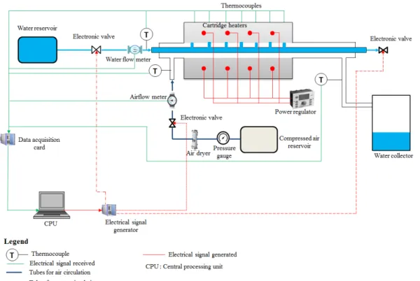
The experimental bench consists principally of an instrumented stainless steel block (grade 316L) referred to as the test segment with dimensions 200×100×90 mm and a cylindrical channel of a ∅30 mm diameter bored centrally along its length (Fig. 2). The distance between the surface of interest and the channel (Fig. 3a) is 30 mm. For heating purposes, 8 circular holes with a diameter of 10 mm were bored along the test segment’s width in order to create space for the placement of the cylindrical cartridge heaters. The test segment’s internal temperature was monitored by 9 type K thermocouples with a diameter of 3 mm inserted at a depth of 50 mm along the test segment’s width (Fig. 3a). The test segment’s top surface is representative of the mould/part interface and is monitored by 25 type K thermocouples with a diameter of 0.5 mm as illustrated on Fig. 3b. The red dots represent the hot junctions of the thermocouples while the black lines represent the positions of the grooves used to hold the thermocouples in place. For the channeling of the air flow, water vapour and the remaining liquid water, 2 cylindrical quartz tubes with a diameter of ∅33/30 mm and length of 400 mm are attached to both ends of the central channel. The air passes through a compressed air dryer before flowing through the cooling channel (Fig. 2). The joints are rendered airtight by the use of a silicon seal. A perforated stainless tube with a length of 1000 mm and diameter of ∅12/10 mm is inserted along the central axis of the test segment’s channel and of both cylindrical tubes attached to the test segment’s sides. The perforations were made on the side of the tube facing the top surface (opposing gravity) of the test segment’s channel and consist of 7 orifices with a diameter of ∅1 mm. There’s a distance of 30 mm separating adjacent orifices with the first orifice being at a distance of 10 mm from the channel’s entrance. All the sides of the test segment are insulated by a 50 mm thick fiberglass material as illustrated on Fig. 4. For the monitoring of the fluid temperatures, thermocouples are inserted into the entrances and exits of the central tube and the cylindrical glass tubes. The temperature of the water entering the central tube is measured by a 3 mm rigid type K thermocouple whose hot junction is positioned at the center of the flow (Fig. 2). The same approach is used to measure the temperature of the air entering the quartz tube attached to the entrance of the test segment’s channel and to measure the temperature of the mixture of air, water vapour and liquid water exiting the test segment (Fig. 2). All temperature acquisitions are made centrally on a National Instruments® acquisition card (NI TB-4353) inserted into an NI PXIe-1073 chassis and the temperatures are monitored in real time on LABVIEW®.
The flow rates of the water and air are controlled by electronic valves installed at the entrances of the central steel tube and the quartz tube respectively. The flow rate of the water is controlled by a type 6223 Burkert electronic valve while the flow rate of the air is controlled by a type 3280 Burkert electronic valve. In order to measure the flow rates of both fluids, flow meters are installed after the electronic valves. The flow rate of the
4 water is measured by an ultrasonic flow meter (Atrato 740-V10-D) while that of the air is measured by an SMC PFMB7102 flow meter. Both electronic valves are controlled by (0 - 10 V) signals generated by an NI-6229 National Instruments® command card controlled from LABVIEW®.
During each experiment, the test segment is heated for approximately 1200 s by a total power of 2160 W to a temperature of 593 K and allowed to cool naturally to the desired initial cooling temperature of 573 K. This approach improves upon the test segment’s temperature homogeneity before the cooling phase is commenced (maximum temperature difference of 6 K on the test segment’s surface) due to the transfer of heat from the hotter zones to the colder zones. Once the required initial temperature is attained, the cooling phase is initiated by releasing both fluids into their respective tubes, done by opening the electronic valves that regulate their flow rates. The exit of the central tube is closed by an SMC VXED2140 electronic valve in order to generate a higher pressure within the tubes and to direct all the water towards the orifices.
Fig. 2 Schematic illustration of experimental bench
Uncertainty analysis
The parametric studies involved 5 water flow rates and 5 air flow rates. The exact values of the water flow rates expressed as the mean and the standard deviation (SD) of the values measured over the duration of the experiments are displayed on Table 1. The values of the air flow rates on the table are also time averaged with their standard deviations ranging from (0.04 – 0.1) g/s. For all the experiments, the temperature of the water
stayed within the range of (289 - 294) K while the temperature of the air stayed within the range of (294 - 296) K.
200
5
a) b)
Fig. 3 Illustration of the dimensions and the positions of the cartridge heaters and the thermocouples, a) Side view, b) Top view
a) b)
Fig. 4 Images of test segment: a) View of instrumented test segment from above, b) View of insulated test segment
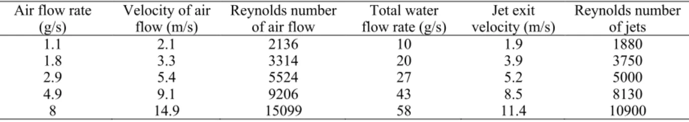
The uncertainty on the water flow rate measurements was estimated by the manufacturers at 1% over the flow range (0.3 – 83) g/s while that on the air flow rate measurements was estimated at 3% over the flow range of (0.1 – 9.8) g/s. The temperature measurement uncertainty linked to the temperature acquisition system (cold junction compensation and thermal EMF) was estimated at ±0.38 K while the uncertainty of the type K thermocouples is the higher of ±2.5 K or ±0.75 % of the measured value according to the manufacturer. Assuming a confidence interval of 95 %, this value was divided by 1.96 to give a standard uncertainty of ±1.28 K. This gives us a global uncertainty on the temperature measurements of ±1.66 K Table 2 shows us the Reynolds numbers and velocities of the air flow and the water jets. The flow rate of each individual jet was measured by means of a chronometer and a scale balance and the flow rates measured were found to lie within a range of ±10% of the reference value. In the calculation of the jet exit velocities and Reynolds numbers, the mean of the flow rates of the 7 individual jets was used. The uncertainties on the calculated parameters obtained by propagating the uncertainties on the measured parameters are presented on Table 3.
Table 1 Exact values of the water flow rates for the different sets of experiments conducted Water flow rate (g/s)
10 20 27 43 58
Air flow
rate (g/s) Mean value SD Mean value SD Mean value SD Mean value SD Mean value SD 1.1 9.3 1.8 18.7 3.3 26.8 3.0 45.3 5.0 53.8 5.0 1.8 9.0 1.8 20.0 1.8 27.2 4.5 46.0 4.5 60.8 5.3 2.9 11.3 1.8 20.2 2.2 26.8 3.8 44.3 5.3 60.0 5.7 4.9 9.5 1.2 19.8 2.7 25.8 3.2 45.2 4.5 58.3 5.7 8 11.3 1.3 20.3 1.7 25.0 3.0 43.7 4.2 55.5 5.8
Table 2 Reynolds numbers of the fluids for the ranges of flow rates tested Air flow rate
(g/s) Velocity of air flow (m/s) Reynolds number of air flow flow rate (g/s) Total water velocity (m/s) Jet exit Reynolds number of jets
1.1 2.1 2136 10 1.9 1880
1.8 3.3 3314 20 3.9 3750
2.9 5.4 5524 27 5.2 5000
4.9 9.1 9206 43 8.5 8130
8 14.9 15099 58 11.4 10900
Table 3 Uncertainty on calculated parameters
6
Jet exit velocity ±1.01
Reynolds number of jets ±7.69
Velocity of air flow ±4.32
Reynolds number of air flow ±4.91 2.2 Methods
2.2.1 Evaluation of the temperature homogeneity of the test segment’s top surface along its length
The temperature homogeneity along the test segment’s length was evaluated by taking the mean and the maximum values of all the temperature differences between the 13 centrally aligned thermocouples at each time step. The heterogeneities in temperature brought about by the heating phase were accounted for by subtracting the initial temperature value at the onset of cooling for each thermocouple from all the subsequent temperature measurements (Eq. (1)) before proceeding to the calculation of the mean (Eq. (2)) of the temperature differences at each time step.
Ti (t) = Yi (t) – Yi (t=0) (1)
Mean (E '(t)) = ∑,60/,∑,-./01,( |30(4)53.(4)| )
7 (2)
where i = thermocouple number starting from the left and n = total number of temperature differences
The spatial mean temperature of the entire segment surface was obtained by averaging all the 25 temperature measurements made on the surface (Fig. 3b).This mean was used to monitor the temperature and the cooling speed of the entire surface.
2.2.2 Model predictive control of the cooling speed of the test segment’s top surface
Model predictive control (MPC) is an advanced control method that can be used to predict the behavior of linear and non-linear systems. One of the major advantages of model predictive control when compared to other control techniques such as PID (Proportional Integral Derivative), LQR (Linear Quadratic Regulator) and LQG (Linear Quadratic Gaussian) is the fact that it can be used to optimize multivariable objective functions with or without constraints. MPC also works best for systems with relatively high response times.
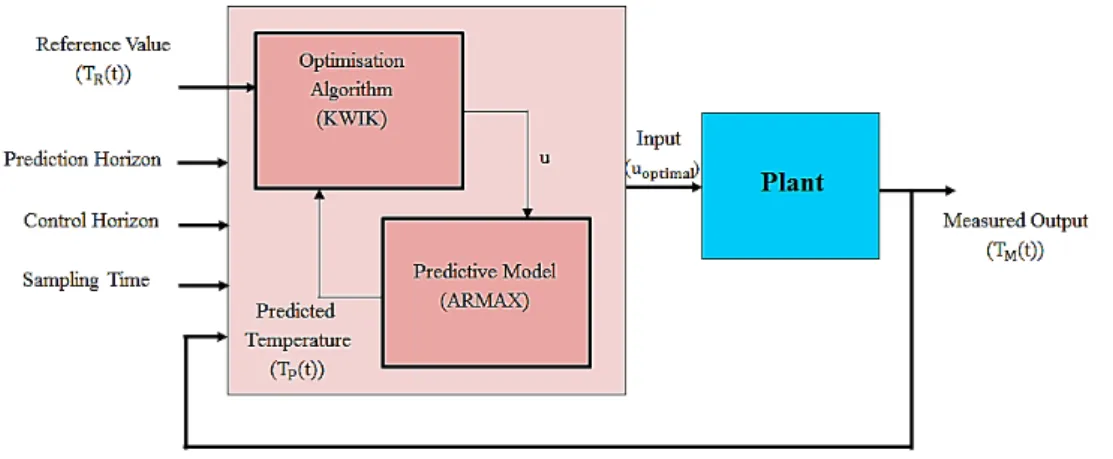
Figure 5 shows us the operating principles of MPC which consists principally of an optimization algorithm and a predictive model. MPC seeks to minimize the errors between the values predicted by the predictive model and the reference values which are imposed. It does this by optimizing a sequence of plant inputs by means of an optimization algorithm. The measured outputs from the plant are also used by the MPC in real time in order to update its current state. The objective function optimized by the algorithm is illustrated by Eq. (3) while Eq. (4) illustrates the sequence of the plant inputs. Some other important parameters to take into account when setting up MPC are the prediction horizon, the control horizon and the sampling time. The selection criteria for these different parameters are explained by Alberto et al. [18]. For this study, a prediction horizon of 25, control horizon of 2, and sampling time of 2 s were used.
7 J(u:) = < < =
w?,A
sA CTE,A(k + i) − TJ,A(k + i)KL M J NOP 7 QOP (3) z:3= [u(k)3 u(k + 1)3 … u(k + hp − 1)3] (4)
Where k = current control interval, z = quadratic program (QP) decision, n = number of plant output variables, sj = scale factor of jth plant output in engineering units, wi,j = tuning weight for jth plant output at ith prediction
time step (dimensionless), p = prediction horizon
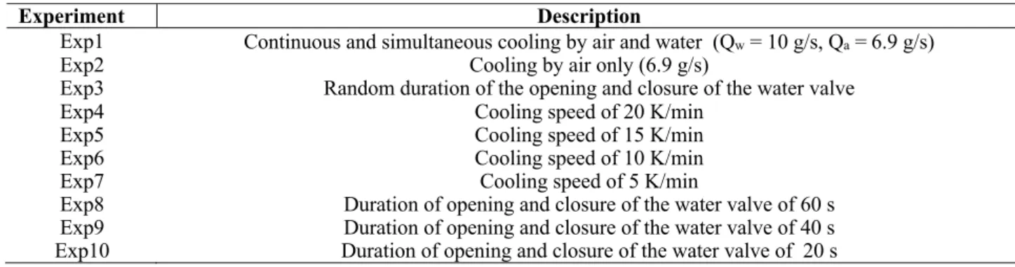
In this study, model predictive control was applied to control the cooling speed of the test segment’s surface by optimizing the sequence of the opening and the closure of the electronic water valve. The predictive model used was a data driven polynomial model known as ARMAX [19] while the optimization algorithm used by the MPC is known as KWIK [20]. Both the predictive model and the MPC are contained in the model predictive toolbox and the system identification toolbox of MATLAB® which was used for this study. Given the fact that ARMAX is a data driven model, the model had to be fed with experimental data (Table 4) that is representative of the system’s dynamics (heat transfer within the test segment). Some of the data was used to estimate the model parameters (Fig. 6) while the rest of the data was used to validate the model created. The cooling speeds of Exp4 - Exp7 (Table 4) were obtained from a simpler automated cooling approach illustrated by Fig.7 where the spatial mean surface temperature of the test segment’s surface (spatial mean of 25 temperature measurements) is compared to a reference temperature at each time interval and the opening and closure of the water valve is determined by the difference between both temperatures. The limitation of this approach is the fact that the heat diffusion response time of the test segment isn’t taken into account. Hence the measured temperature tends to deviate from the reference temperature due to the late closure of the water valve. The input takes a value of either 0 or 1 where 0 represents a closed water valve and 1 represents an open water valve. The orders of the different polynomials of the ARMAX model used are [7 5 4 3]. These values were determined by optimizing the objective function represented by Eq. (5).
RSE =Y∑ ∑ ZT[\]^,_− T`\]^,_a M bcdefg bOh Ph ij`Ok (5)
Table 4 Summary of different experiments used to determine the optimal orders and coefficients of the predictive model
Experiment Description
Exp1 Continuous and simultaneous cooling by air and water (Qw = 10 g/s, Qa = 6.9 g/s) Exp2 Cooling by air only (6.9 g/s)
Exp3 Random duration of the opening and closure of the water valve Exp4 Cooling speed of 20 K/min
Exp5 Cooling speed of 15 K/min Exp6 Cooling speed of 10 K/min
Exp7 Cooling speed of 5 K/min
Exp8 Duration of opening and closure of the water valve of 60 s Exp9 Duration of opening and closure of the water valve of 40 s Exp10 Duration of opening and closure of the water valve of 20 s
8 Fig. 6 Experimental data used to determine the predictive model’s coefficients
Fig.7 On/Off cooling speed control algorithm without MPC
The results of the evaluation of the accuracy of the model created are illustrated on Fig. 8. The accuracy of the model was evaluated by taking the root mean square error (RMSE) and the absolute value of the temperature difference (dT) between the measured output and the model output at each time interval evaluated by Eq. (6) and Eq. (7) respectively. We observe from Fig. 8 that the accuracy of the model created is satisfactory for the desired application. RMSE = Y∑ Z3l(4)5 3m(4)a 6 _n _/o 7 (6) dT(t) = pT[(t) − TJ(t)p (7)
9 Fig. 8 ARMAX model validation results
3 Results and discussion
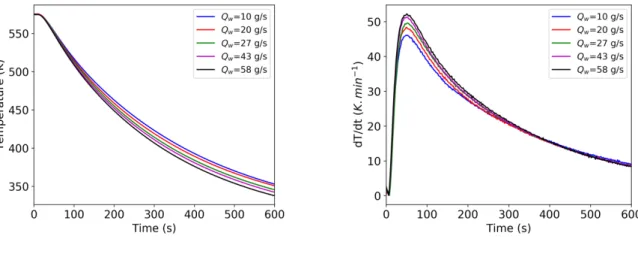
3.1 Influence of the flow rates of the fluids on the cooling speed of the test segment’s top surface The effect of varying the flow rate of the water and that of the air was studied. Fig. 9 shows us the evolution of the spatial mean temperature (Fig. 9a) and of the cooling speed (Fig. 9b) of the test segment’s top surface with respect to time for different water flow rates and a constant air flow rate of 1.8 g/s while Fig. 10 shows us the evolution of the spatial mean temperature (Fig. 10a) and of the cooling speed (Fig. 10b) for different air flow rates and a constant water flow rate of 27 g/s. For all the scenarios tested, it can be observed that the cooling speed peaks after approximately 50 s and then reduces progressively over time. A possible explanation for this is the change of boiling regimes from the transition boiling regime to the nucleate boiling regime. The same transition can be seen in the literature [21] for a similar temperature range.
10
a) b)
Fig. 9 Effect of the flow rate of the water on the cooling speed of test segment’s top surface for a constant air flow rate of 1.8 g/s: a) Evolution of the surface temperature with respect to time, b) Evolution of surface cooling speed with respect to time
a) b)
Fig. 10 Effect of the air flow rate on the cooling speed of test segment’s top surface for a constant water flow rate of 27 g/s: a) Evolution of the surface temperature with respect to time, b) Evolution of surface cooling speed with respect to time
The progressive decrease in the cooling speed can be explained by the fact that the heat flux at the impinged surface is dependent on its temperature [20-21] and decreases progressively with the decrease in temperature. Another observation is that there’s a slight increase in the cooling speed of the test segment’s surface with an increase in the flow rate of the water (Fig. 9) with a maximum cooling speed of 46 K/min for a 10 g/s flow rate and maximum cooling speed of 52 K/min for a flow rate of 58 g/s. This can be explained by the fact that increasing the flow rate of the water increases jet velocity for fixed orifice diameters and a positive correlation can be found between jet velocity and heat flux [23]. It can also be observed that the cooling speeds for all the flow rates converge at a time of about 300 s. At this point, the temperature of the channel’s surface is less than 373 K [24] and there’s no phase change of the water. This means that in the absence of phase change (boiling and evaporation) increasing the flow rate of the water beyond the lowest value of 10 g/s has no major impact on the cooling speed of the test segment’s top surface. Furthermore, there’s no significant difference between the cooling speeds obtained for water flow rates of 43 g/s and 58 g/s. This could indicate that increasing the water flow rate further beyond this value wouldn’t lead to a significant increase in the cooling speed. Additionally, it can be observed from Fig. 10 that the air flow has no significant effect on the cooling speed of the test segment’s top surface. Similar trends were observed for the other combinations of water and air flow rates.
3.2 Influence of the flow rates of the fluids on the temperature homogeneity of the test segment’s top surface along its length
For different flow parameters, the homogeneity of the temperature along the length of the test segment’s surface was evaluated by Eq. (2) and the maximum temperature difference among all the temperature differences calculated for a given time step was also analyzed. The results obtained for a water flow rate of 10 g/s are
11 illustrated on Fig. 11. It can be observed from Fig. 11 that increasing the air flow rate tends to worsen the temperature homogeneity along the length of the test segment.
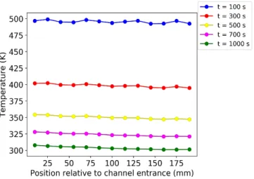
Figure 12 shows us the temperature distribution along the length of the test segment’s surface at different times for a water flow rate of 10 g/s and an air flow rate of 1.1 g/s. We can observe from the figure that the temperature distribution is relatively uniform except for the presence of some temperature peaks along the surface during the first 500 s of cooling indicated by the red broken lines. These peaks are caused by the presence of the cartridge heaters at those positions. The difference in thermal properties between the cartridge heaters and the test segment coupled with the thermal contact resistance between them slows down the transfer of heat from the test segment’s surface.
a) b)
Fig. 11 Influence of the air flow rate on the homogeneity in temperature along the test segment’s length for a water flow rate of 10 g/s: a) Evolution of the mean temperature difference with respect to time, b) Evolution of the maximum temperature difference with respect to time
Fig. 12 Temperature distribution along length of test segment’s surface for Qw=10 g/s and Qa=1.1 g/s
Figures 13 and 14 evaluate the temperature uniformity along the length of the test segment’s surface for a water flow rate of 27 g/s and different air flow rates while Fig. 15 and Fig. 16 evaluate the temperature uniformity for a water flow rate of 58 g/s and different air flow rates. For the higher water flow rates of 26.7 g/s (Fig. 13) and 58 g/s (Fig. 15), increasing the air flow rate has a lesser influence on the temperature homogeneity of the test segment’s top surface. This could be due to the fact that for the lower water flow rate of 10 g/s, the more the air flow rate is increased, the more the jets tend to tilt under the force of the air flow, hence the water film formed on the channel’s surface during jet impingement is not uniformly distributed along the impinged surface. The temperature distribution at different times for the water flow rates of 27 g/s (Fig. 14) and 58 g/s (Fig. 16) is similar to that obtained with a water flow rate of 10 g/s.
12
a) b)
Fig. 13 Influence of the air flow rate on the homogeneity in temperature along the test segment’s length for a water flow rate of 27 g/s: a) Evolution of the mean temperature difference with respect to time, b) Evolution of the maximum temperature difference with respect to time
Fig. 14 Temperature distribution along length of test segment’s surface for Qw=27 g/s and Qa=1.1 g/s
a) b)
Fig. 15 Influence of the air flow rate on the homogeneity in temperature along the test segment’s length for a water flow rate of 58 g/s: a) Evolution of the mean temperature difference with respect to time, b) Evolution of the maximum temperature difference with respect to time
13 Fig. 16 Temperature distribution along length of test segment’s surface for Qw=58 g/s and Qa=1.1 g/s
A noticeable advantage of this cooling approach is the fact that the temperature homogeneity doesn’t get worse over time and the mean temperature difference happens to stabilize within the range of (1-2.5) K and the maximum temperature difference within the range of (2.5-6) K for a water flow rate of 10 g/s and air flow rate of 1.1 g/s. This is not the case when cooling is done via the traditional channel flow approach for the reason that the fluid tends to heat up as it flows through the channel, resulting in the progressive reduction of the heat flux along the channel. Additionally, when boiling is involved, the formation of vapor pockets tends to worsen the heat flux disparity along the channel. This phenomenon was demonstrated by the studies of Tymen et al. [9] and Yin et al. [25]. Due to the reasons stated above, the temperature homogeneity of a tool cooled via the channel flow approach gets worse over time.
3.3 Automatic control of the cooling speed of the test segment’s surface
The test segment was cooled automatically with the MPC designed by the approach described in section 2.2.2. The results obtained were compared to those gotten from the simpler automated cooling approach illustrated on Fig.7. During the automated cooling of the test segment, a constant water flow rate of 10 g/s and air flow rate of 6.9 g/s were used. The air flow control valve was opened permanently for the entire duration of the cooling in order to remove the excess liquid from the channel while the opening of the water valve was controlled by the automated cooling algorithms. The reason for using the lowest water flow rate of 10 g/s for the automated cooling was to limit the cooling speed, especially within the first 120 s, in order to reduce the amplitude of the deviation of the measured temperatures from the reference temperatures during the impingement of the water jets. Different cooling ramps were imposed and the results obtained for cooling ramps of 5 K/min, 10 K/min, 15 K/min, 20 K/min and 25 K/min are illustrated on Fig. 17, Fig. 18, Fig. 19, Fig. 20 and Fig. 21 respectively.
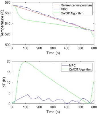
14 Fig. 17 Cooling ramp of 5 K/min
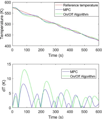
15 Fig. 19 Cooling ramp of 15 K/min
16 Fig. 21 Cooling ramp of 25 K/min
We observe from the figures above that compared to the simpler On/Off cooling algorithm, the MPC improves upon the accuracy of the measured temperatures with respect to the reference cooling ramp imposed. Table 5 summarizes the RMSEs obtained for the different algorithms and cooling ramps used. Another observation is that for the highest cooling speeds of 20 K/min and 25 K/min, due to physical cooling speed limitations, after a certain duration (350 s), the cooling speed of the test segment is unable to keep up with the ramp imposed. The reason for this is that the heat flux at the channel surface isn’t high enough to maintain the desired speed. Such limitations can be accounted for at the mould design stage by choosing the appropriate material and mass for the mould, the number of cooling channels and the distance between the channels and the mould/part interface.
Table 5 RMSE in K for different automated cooling algorithms and cooling ramps Cooling ramp (K/min)
Automated cooling approach 5 10 15 20 25 MPC 1.98 5.49 3.57 4.38 15.36 On/Off Algorithm 11.43 10.35 5.38 6.76 18.63 4 Conclusion
An approach to automatically and accurately control the cooling speed and the temperature distribution along a mould/part interface is proposed. The simultaneous use of multiple impinging water jets and a cross air flow is used instead of channel flow in order to improve upon the temperature homogeneity along the length of the test segment. These studies revealed that:
• By using a combination of water jets and a cross air flow, a homogenous surface temperature along the length of a mould segment can be maintained. For the specimen studied, the mean temperature was able to be maintained within the range of (1 – 2.5) K while the maximum temperature difference was maintained within the (2.5 - 6) K range during the entire duration of the cooling
17 under certain fluid flow conditions. This isn’t the case with the traditional cooling approach of channel flow where the temperature homogeneity gets worse over time.
• Model predictive control can be used to accurately (within ± 5 K of the imposed cooling ramp) control the cooling speed of a mould segment under boiling conditions within the physical cooling speed limitations of the system. The major advantage of this approach is that it can be adapted to a variety of cooling systems by using appropriate experimental measurements that represent the dynamics of the system for the construction of the data driven model (predictive model).
• During the simultaneous use of water jets and a cross air flow for heat extraction, increasing the air flow rate has no significant effect on the cooling speed of the test segment’s top surface. However, for relatively lower water flow rates (<16.7 g/s for the experimental conditions described), increasing the air flow rate tends to worsen the temperature homogeneity of the test segment’s top surface.
In perspective, the application of this technology on a complete mould prototype with multiple channels and a real part could be studied.
Acknowledgement
This research was supported by financing from the PERFORM program of the Institut de Recherche Technologique Jules Verne. The authors are grateful to Yannick Madec and Erwann Paviot for their help during the fabrication and assembly of the experimental bench.
Nomenclature d Diameter, m Q Flow rate, kg/s g Gravity, m/s2 u Input v Kinematic viscosity, m2/s MPC Model predictive control
Rea Reynolds number of air flow, q(rsv5tu) Rej Reynolds number jets, qtw
v
RMSE Root mean square error, K RSE Root square error, K
SD Standard deviation, kg/s T Temperature, K
t Time, s
v Velocity of the flow, m/s
Y Unadjusted temperature measurement, K
Subscripts
a Air
c Diameter of channel
e External diameter of central tube j Diameter of jet orifice
M Measured output temperature, K p Predicted temperature, K R Reference temperature, K References
[1] Gombos, Z. J., McCutchion, P., and Savage, L., 2019, “Thermo-Mechanical Behaviour of Composite Moulding Compounds at Elevated Temperatures,” Composites Part B: Engineering, 173, p. 106921. DOI: https://doi.org/10.1016/j.compositesb.2019.106921
[2] Chen, X., Lam, Y. C., and Li, D. Q., 2000, “Analysis of Thermal Residual Stress in Plastic Injection Molding,” Journal of Materials Processing Technology, 101(1), pp. 275–280.
DOI: https://doi.org/10.1016/S0924-0136(00)00472-6
[3] Wang, T.-H., and Young, W.-B., 2005, “Study on Residual Stresses of Thin-Walled Injection Molding,” European Polymer Journal, 41(10), pp. 2511–2517.
18 [4] Arrizubieta, J. I., Cortina, M., Ostolaza, M., Ruiz, J. E., and Lamikiz, A., 2019, “Case Study: Modeling of the Cycle Time Reduction in a B-Pillar Hot Stamping Operation Using Conformal Cooling,” Procedia Manufacturing, 41, pp. 50–57.
DOI: 10.1016/j.promfg.2019.07.028
[5] Deepika, S. S., Patil, B. T., and Shaikh, V. A., 2020, “Plastic Injection Molded Door Handle Cooling Time Reduction Investigation Using Conformal Cooling Channels,” Materials Today: Proceedings.
DOI: 10.1016/j.matpr.2019.11.316
[6] Dimla, D. E., Camilotto, M., and Miani, F., 2005, “Design and Optimisation of Conformal Cooling Channels in Injection Moulding Tools,” Journal of Materials Processing Technology, 164–165, pp. 1294– 1300.
DOI:10.1016/j.jmatprotec.2005.02.162
[7] Marques, S., Souza, A. F. de, Miranda, J., and Yadroitsau, I., 2015, “Design of Conformal Cooling for Plastic Injection Moulding by Heat Transfer Simulation,” Polimeros, 25, pp. 564–574.
DOI: https://doi.org/10.1590/0104-1428.2047
[8] Yan, J., Bi, Q., Liu, Z., Zhu, G., and Cai, L., 2015, “Subcooled Flow Boiling Heat Transfer of Water in a Circular Tube under High Heat Fluxes and High Mass Fluxes,” Fusion Engineering and Design, 100, pp. 406–418.
DOI: https://doi.org/10.1016/j.fusengdes.2015.07.007
[9] Tymen, G., Allanic, N., Sarda, A., Mousseau, P., Plot, C., Madec, Y., and Caltagirone, J. P., 2018, “Temperature Mapping in a Two-Phase Water-Steam Horizontal Flow,” Experimental Heat Transfer, 31(4), pp. 317–333.
DOI: https://doi.org/10.1080/08916152.2017.1410505
[10] Incropera, F. P., and Ramadhyani, S., 1994, “Single-Phase, Liquid Jet Impingement Cooling of High-Performance Chips,” Cooling of Electronic Systems, S. Kakaç, H. Yüncü, and K. Hijikata, eds., Springer Netherlands, Dordrecht, pp. 457–506.
DOI: https://doi.org/10.1007/978-94-011-1090-7_21
[11] Karwa, N., Gambaryan-Roisman, T., Stephan, P., and Tropea, C., 2011, “Experimental Investigation of Circular Free-Surface Jet Impingement Quenching: Transient Hydrodynamics and Heat Transfer,” Experimental Thermal and Fluid Science, 35(7), pp. 1435–1443.
DOI: 10.1016/j.expthermflusci.2011.05.011
[12] Wei, T.-W., Oprins, H., Cherman, V., Plas, G. V. der, Wolf, I. D., Beyne, E., and Baelmans, M., 2019, “Experimental Characterization and Model Validation of Liquid Jet Impingement Cooling Using a High Spatial Resolution and Programmable Thermal Test Chip,” Applied Thermal Engineering, 152, pp. 308– 318.
DOI: https://doi.org/10.1016/j.applthermaleng.2019.02.075
[13] Whelan, B. P., and Robinson, A. J., 2009, “Nozzle Geometry Effects in Liquid Jet Array Impingement,” Applied Thermal Engineering, 29(11), pp. 2211–2221.
DOI: https://doi.org/10.1016/j.applthermaleng.2008.11.003
[14] Lee, S. G., Kaviany, M., and Lee, J., 2018, “Quench Subcooled-Jet Impingement Boiling: Two Interacting-Jet Enhancement,” International Journal of Heat and Mass Transfer, 126, pp. 1302–1314. DOI: 10.1016/j.ijheatmasstransfer.2017.05.081
[15] Teamah, M. A., and Khairat, M. M., 2015, “Heat Transfer Due to Impinging Double Free Circular Jets,” Alexandria Engineering Journal, 54(3), pp. 281–293.
DOI: https://doi.org/10.1016/j.aej.2015.05.010
[16] Menges, G., Michaeli, W., and Mohren, P., 2001, How to Make Injection Molds, Carl Hanser Verlag GmbH & Co. KG.
DOI: https://doi.org/10.3139/9783446401808.fm
[17] N. Rao, and Schumacher, G., 2004, Design Formulas for Plastics Engineers, Hanser.
[18] Alberto Bemporad, Ricker, N. L., and Morari, M., 2020, “Model Predictive Control Toolbox - User’s Guide.”
[19] Simpkins, A., 2012, “System Identification: Theory for the User, 2nd Edition (Ljung, L.; 1999) [On the Shelf],” IEEE Robotics Automation Magazine, 19(2), pp. 95–96.
DOI: 10.1109/MRA.2012.2192817
[20] Schmid, C., and Biegler, L. T., 1994, “Quadratic Programming Methods for Reduced Hessian SQP,” Computers & Chemical Engineering, 18(9), pp. 817–832.
DOI: 10.1016/0098-1354(94)E0001-4
[21] Ishigai, S., and Nakanishi, S., 1978, “Boiling Heat Transfer for a Plane Water Jet Impinging on a Hot Surface,” Proceedings of the International Heat Transfer Conference, Toronto, Canada, August 7-11, 1978, pp. 445–450.
[22] Karwa, N., Gambaryan-Roisman, T., Stephan, P., and Tropea, C., 2011, “Experimental Investigation of Circular Free-Surface Jet Impingement Quenching: Transient Hydrodynamics and Heat Transfer,” Experimental Thermal and Fluid Science, 35(7), pp. 1435–1443.
19 [23] Karwa, N., and Stephan, P., 2013, “Experimental Investigation of Free-Surface Jet Impingement
Quenching Process,” International Journal of Heat and Mass Transfer, 64, pp. 1118–1126. DOI: 10.1016/j.ijheatmasstransfer.2013.05.014
[24] Agyeman, E., Mousseau, P., Sarda, A., Edelin, D., and Lecointe, D., 2019, “Etude Thermique Expérimentale de l’impact d’un Jet d’eau sur une Surface Métallique Concave,” Proceedings of the Colloque International Franco-Québécois; Baie St-Paul, Québec, Canada, June 16-20, 2019.
https://hal.archives-ouvertes.fr/hal-02340513/
[25] Yin, S., Zhang, J., Tong, L., Yao, Y., and Wang, L., 2013, “Experimental Study on Flow Patterns for Water Boiling in Horizontal Heated Tubes,” Chemical Engineering Science, 102, pp. 577–584.
20 List of tables
Table 1 Exact values of the water flow rates for the different sets of experiments conducted 5 Table 2 Reynolds numbers of the fluids for the ranges of flow rates tested 6 Table 3 Uncertainty on calculated parameters 6 Table 4 Summary of different experiments used to determine the optimal orders and coefficients of the
predictive model 7
Table 5 RMSE in K for different automated cooling algorithms and cooling ramps 16
21
Fig. 1 Illustration of the cooling approach 3
Fig. 2 Schematic illustration of experimental bench 4 Fig. 3 Illustration of the dimensions and the positions of the cartridge heaters and the thermocouples, a) Side
view, b) Top view 5
Fig. 4 Images of test segment: a) View of instrumented test segment from above, b) View of insulated test
segment 5
Fig. 5 Schematic illustration of model predictive control 7 Fig. 6 Experimental data used for the determination of the predictive model’s coefficients 8 Fig.7 On/Off cooling speed control algorithm without MPC 8
Fig. 8 ARMAX model validation results 9
Fig. 9 Effect of the flow rate of the water on the cooling speed of test segment’s top surface for a constant air flow rate of 1.8 g/s: a) Evolution of the surface temperature with respect to time, b) Evolution of surface cooling speed with respect to time 10 Fig. 10 Effect of the air flow rate on the cooling speed of test segment’s top surface for a constant water flow
rate of 27 g/s: a) Evolution of the surface temperature with respect to time, b) Evolution of surface
cooling speed with respect to time 10
Fig. 11 Influence of the air flow rate on the homogeneity in temperature along the test segment’s length for a water flow rate of 10 g/s: a) Evolution of the mean temperature difference with respect to time, b) Evolution of the maximum temperature difference with respect to time 11 Fig. 12 Temperature distribution along length of test segment’s surface for Qw=10 g/s and Qa=1.1 g/s 11 Fig. 13 Influence of the air flow rate on the homogeneity in temperature along the test segment’s length for a
water flow rate of 27 g/s: a) Evolution of the mean temperature difference with respect to time, b) Evolution of the maximum temperature difference with respect to time 12 Fig. 14 Temperature distribution along length of test segment’s surface for Qw=27 g/s and Qa=1.1 g/s 12 Fig. 15 Influence of the air flow rate on the homogeneity in temperature along the test segment’s length for a
water flow rate of 58 g/s: a) Evolution of the mean temperature difference with respect to time, b) Evolution of the maximum temperature difference with respect to time 12 Fig. 16 Temperature distribution along length of test segment’s surface for Qw=58 g/s and Qa=1.1 g/s 13
Fig. 17 Cooling ramp of 5 K/min 14
Fig. 18 Cooling ramp of 10 K/min 14
Fig. 19 Cooling ramp of 15 K/min 15
Fig. 20 Cooling ramp of 20 K/min 15