Science Arts & Métiers (SAM)
is an open access repository that collects the work of Arts et Métiers Institute of
Technology researchers and makes it freely available over the web where possible.
This is an author-deposited version published in: https://sam.ensam.eu Handle ID: .http://hdl.handle.net/10985/8340
To cite this version :
Frédéric CHARPENTIER, Alex BALLU, Jérôme PAILHES - A scientific point of view of a simple industrial tolerancing process - Procedia Engineering p.10 p. - 2011
Any correspondence concerning this service should be sent to the repository Administrator : archiveouverte@ensam.eu
12
thCIRP Conference on Computer Aided Tolerancing
A scientific point of view
of a simple industrial tolerancing process
F. Charpentier
a, A. Ballu
a*, J. Pailhes
baUniv. Bordeaux, I2M, UMR 5295, 351 Cours de la Libération, F-33400 Talence, France. bArts et Metiers ParisTech, I2M, UMR 5295, F-33400 Talence, France
Abstract
The purpose of this paper is to decipher the process of modelling driving to the product behaviour simulation. A simple example of simulation, tolerance stackup, allows illustrating this process. The tolerance stackup is used daily in industry, however, designers do they know exactly what they do? Are they aware of the assumptions they are introducing? To answer to these questions, concepts of GeoSpelling and of GPS ISO standards such as skin model, operations, operators and other concept are introduced such as finite and infinite models.
Keywords: Tolerancing analysis; GeoSpelling; GPS; activity model;
1. Introduction
Tolerancing has been highly developed since the 90s by the research, standardization and industrial activities. The purpose of this paper is to decipher the tolerancing methods employed in the industry from a simple example of 1D tolerance chain. Dimensional tolerancing is a long-standing concern for industry [1]. Tolerance chain and stackup are used daily in industry for at least 50 years.
Many research papers concern this topic. Historically, the mechanical parts have been considered as perfect, because they visually appeared without defects. The part surface is seen as a set of perfect surfaces (plane, cylinder, cone…) in exact situations [2][3][4]. For the past 20 years, research has been focusing on the influence of the orientation defects [5].
Nevertheless, the product design is realised using a nominal geometrical model. This model uses different parameters and design variables such as lengths, masses, inertias and volumes. Each parameter
*Corresponding author. Tel.: +33-5 4000 66 13; fax: +33-5 4000 69 64 E-mail address: alex.ballu@u-bordeaux1.fr
is considered in its nominal state. CAD systems are based on this nominal model. They integrate many powerful simulation tools, for example kinematics, dynamics, structural calculation tools. The nominal geometrical model does not take into account imperfections linked to the real world. However for these applications, using a nominal model is generally sufficient in comparison with the influence of the imperfections on results. The actual parts imperfections are not considered, errors introduced by actual parts imperfections are negligible.
The nominal geometrical model is thus a simple model allowing an easy product design process to succeed in nominal dimensioning. However, the imperfections have an influence, sometimes negligible, sometimes not. The defects during the manufacturing and the “real life” can be the source of dysfunctions. It is particularly the case in assembly and tolerancing analysis. It turns out that modelling of the various geometrical variations has a considerable influence on the deployment of an integrated design activity, i.e. on the product design, on the manufacturing process and on the measurement process.
Ballu & Mathieu developed the language GeoSpelling [6][7] (language for geometrical specification and checking) in the 90’s. The GeoSpelling language is a declaratory language for the specification and the products geometrical verification which has been adopted by the ISO [8]. This language allows a formal representation for design activities, for manufacturing and for control, integrating a realistic sight (realistic geometry) of the parts and mechanical products.
This paper attempts to analyse dimensional stack up tolerance activity with a scientific point of view, i.e. pointing out the different (implicit) assumptions made during this activity. For this purpose, we are using the concept developed for GeoSpelling. This paper aims to propose a framework to define modelling assumptions necessary for the processes and procedures.
2. Models
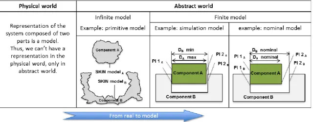
At first, two worlds are considered, the physical world (reality) and the abstract world (models). The term of “skin model” has been introduced by Ballu & Mathieu [7] to name the model of the interface which separates a piece of its environment. It is a conceptual model of parts surfaces defects. The goal is to clearly differentiate between the object physical interface and its model expressed in the form of geometrical surface, i.e.; the skin model. With this expression, it is possible to distinguish the skin of the physical part and the model of the skin, see figure 1.
Modelling aims to simulate the product functioning during all its product life cycle. The parameters number of the used model is finite to be able to simulate or calculate it. Taking into account an infinite number of parameters is impossible on a computer or elsewhere. However, to take into account the real world tends to take into account an infinite number of parameters. Consequently, the distance between the simulation and the real word generates the fact that modelling and simulation of a physical system are not unique and are never perfect. But, these activities must allow to have the best description of physical phenomena. In this article, we distinguish different types of models, Figure 1.
2.1. Finite and infinite models
Concepts of finite model and infinite model are distinguished primarily because these concepts are linked to an invariant criterion. The criterion is based on the number of parameters of a model. This number may be larger or smaller and can even be conceptually infinite. A plane has three positional parameters, a straight line, four parameters, geometry defined in CAD, n parameters, a profile measured with a profilometer, x parameters.
Fig. 1. Physical/abstract world, infinite/finite models.
The number of parameters does not vary according to the designers or modellers because it mostly depends on the knowledge of science and technology. In consequence, this criterion is as an objective criterion.
2.1.1. Infinite model
An infinite model is identified by an infinite set of parameters. For example, the "skin model", or model of the real surface of the part has an infinite number of parameters. This type of model does not allow any identification. Indeed, to identify a skin portion like a nominally plane feature, it is necessary to make a set of operations which will be described later. In the field of physics, a field of contact pressure between two solids is, a priori, arbitrary in the sense that it is defined with an infinite number of parameters.
Note - an infinite model does not allow any identification. At this modelling level, simulation is not possible.
Note - the criterion to distinguish finite and infinite models is objective, it does not depend on the activity, the designer or the modeller.
2.1.2. Finite model
A finite model is identified by a finite set of parameters. For example, a plane is defined by a finite number of parameters. Its description by its equation is used to identify the relevant parameters (finite in number) necessary for its definition. In the field of physics, for example, a uniform pressure field or linear contact between two solids is characterized by a finite number of parameters.
Note - a nominal model is a finite model.
Note - a finite model allows simulation and calculation.
2.2. Primitive and simulation models 2.2.1. Primitive model
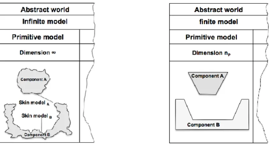
The primitive model is an abstraction of reality made by the designer to model an activity. There may be different primitive models based on assumptions realised for different design activities. This abstraction allows considering the relevant details of things and phenomena of reality according to modelling activities. The primitive model attempts to integrate most defects of actual features (Figure 2a),
Fig. 2. (a) infinite primitive model; (b) finite primitive model
or, according to the designer point of view, to take into account only orientation and position defaults (Figure 2b).
The designer will always seek to define its ideal model, measuring the difference with the primitive model, in order to minimize uncertainties.
2.2.2. Simulation model
The simulation model is a finite model defined by the designer to simulate the system behaviour. In the simulation model, relevant characteristics (parameters, details ...) of things and physical phenomena are considered in order to realise simulation activities. Ideally, the simulation model is the result of a modelling process from the primitive model driving. This process allows having a simpler model which can be used for calculation (that’s why it is finite) and leads to the phenomena quantification. The simplification process is justified by assumptions. The connection between the primitive models and the simulation model involves intermediate models. There may be several simulation models according to the specific simulation activity, the expected accuracy and the designer.
The designer will always seek to define its simulation model, characterizing the “distance” with the primitive model, in order to minimize uncertainties.
2.3. Intermediate models
The link between the primitive model and the simulation model can lead to the introduction of intermediate models. These models have a dimension of the parameters space higher than the dimension of the parameters space of the simulation model. The various intermediate models differ from each other by the number of parameters. The number of intermediate models depends on the “distance” between the primitive model and the simulation model.
Several cases are possible:
Assume that the primitive model is identical to the simulation model. In this case, there are no intermediate models.
Assume that the primitive model is a model with finite number of parameters (Figure 2b) exceeding the number of simulation model parameters. In this case, an intermediate model may be necessary. This intermediate model is a finite model.
Fig. 3. Infinite primitive model, simulation model and intermediate models.
Assume that the primitive model is an infinite model. In this case, several intermediate models may be necessary. The process to simulate the change from the primitive model to the simulation model introduces intermediate models. The number and the definition of intermediate models are defined by the designer. The connection between different models is illustrated at the figure 3 (the intermediate models are not identified in this general figure, but in figure 4).
For the part surface, one can consider the possible different models which differ in the types of geometric defects (size, position, orientation, shape, surface texture). Suppose that the designer considers the model with linear variations (perfect form and orientation, only the position and size of the surfaces vary) as an intermediate model with a dimension ni. The model with linear and angular variations (the
angular variations are added to the linear model variations) becomes an intermediate model with a dimension nj > ni. This remark allows distinguishing the two intermediate models.
Figure 4 shows all the models introduced for a tolerance stack up. These models are detailed in section 3.
3. Linear tolerance stack up
The linear tolerance stack up is daily used in industry. It is based on a simple and well-known method. We use it in the following to illustrate our reflection on the various presented models because of its simplicity and universality. The suggested example is an assembly made up of two parts. The nominal model is presented in figure 5.
A functional analysis makes it possible to define the structuring parameters. The functional decomposition in the physical field is not the object of this paper. Nevertheless, functions make it possible to identify the characteristics and surfaces of the components influencing the assembly.
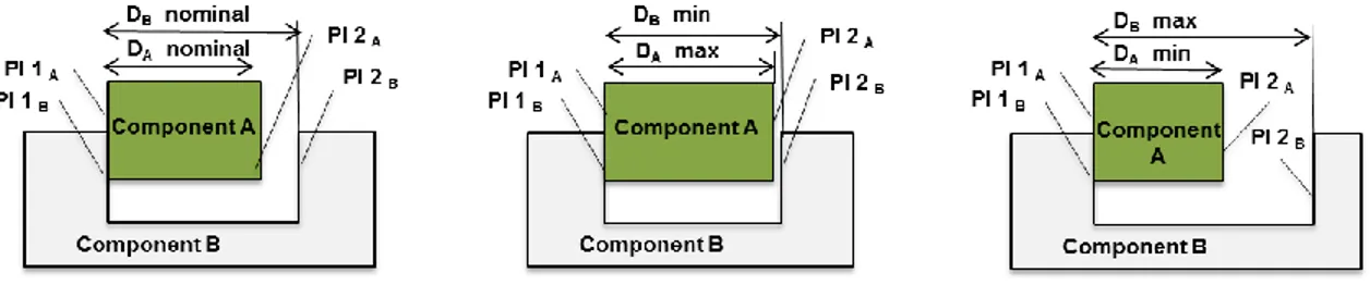
Figure 5 is a nominal representation of the assembly (nominal model). This nominal model is a finite model which corresponds to the design intents and assumptions. This model makes it possible to simulate the system behaviour, but this simulation may be very far away from the “real life” of the system for some functions.
The functional analysis allows characterizing the minimal distances (fig. 5 b) and maximum (fig. 5 c) between the two planes Pl2A and Pl2B. The two planes Pl1A and Pl1B are in contact.
Fig. 5. Models (a) Nominal model, (b) Simulation model with minimum gap, (c) Simulation model with maximum gap
3.1. Primitive model
The primitive model is a model which is an abstraction of reality imagined by the designer to have a reflection about the possible phenomena influencing the product functions. For the same product, there can be several primitive models according to the designer’s assumptions. In order to illustrate this issue, three examples are proposed.
Let us consider that a first designer defines a primitive model (denoted “a”) composed of a set of surfaces with perfect forms and orientations of planes 1 and 2 for each component, see figure 6 a). Only the position and the size of the surfaces vary, i.e. the lengths.
A second designer defines a primitive model (denoted “b”) composed of a set of surfaces only with perfect forms for planes 1 and 2 for each component, see figure 6 b). The position, the orientation and the size of the surfaces vary, i.e. the lengths and the angles.
A last designer is considered, he imagines a primitive model (denoted “c”) which is a surface defined by an infinite number of parameters, see figure 6 c). This feature is named “skin model” in the 17450-1 ISO GPS standard. The position, the orientation, the size, the form and surface texture of the surface vary. These examples define different primitive models according to the designer’s awareness of the reality of the manufacturing defects. According to his willingness he chooses to take into account them or not. From the scientific point of view, the choice to introduce, consciously some defects or not corresponds to the choice of modelling assumptions.
Fig. 6. Examples of primitive models, a) b) and c)
The primitive models of the examples “a” and “b” have the particularity to be composed of canonical surfaces. These primitive models are finite models, a finite number of parameters define the model elements.
The primitive model of the example “c” is a surface feature defined by an infinite number of parameters. It is an infinite model, the “skin model”.
A primitive model is not used to realise a simulation. If it is an infinite model, it is impossible to do it due to the infinite number of parameters. If it is a finite model, the purpose of the primitive model is not to simulate a phenomenon; but to point out the assumptions made to define the simulation model.
3.2. Intermediate models
Normally, the primitive model and the simulation model are different. If they are similar, it means that the designer doesn’t consider other defects than those integrated in the simulation model. Considering they are different, to pass from the primitive to the simulation model, intermediate models are necessary.
3.2.1. Infinite intermediate models
The primitive model of the example “c” is a skin model, i.e. it is an infinite model. In that case, one or several infinite models are necessary to make the connection with the simulation model. Particularly, operations of partition and filtration are used to identify infinite surfaces with bounds (the skin model is a unique surface, including the different functional surfaces of the part without any differentiation).
The ISO 17450-1 standard [8] defines operations of partition and filtration and ISO 22432 standard [9] defines the kind of surfaces or lines obtained. Nevertheless, criteria of partition stay imprecise and depend on the designer.
The operation of partition can be realized from a fitting of the nominal model to the primitive model. For this operation the objective function and the constraints depend on the designer and its simulation activities. The operation of filtration is also defined by the designer according to the characteristics (parameters, details…) relevant to the actual things and phenomena in regard with the simulation activity.
From the primitive model, operations of partition and filtration make it possible to define features for an intermediate model. In our case, these infinite features are nominally plane surfaces, see figure 7.
3.2.2. Finite intermediate model
To make the connection between an infinite model and the simulation model, one or several finite intermediate models may be defined. To define these finite intermediate models different operations can be used such as association, construction and collection as defined in ISO 17450-1.
If the primitive model is a finite model (consequently there are no infinite model), one needs also to define finite intermediate models. In some particular special cases, as example if the primitive model is identical to the simulation one, no finite intermediate model is used.
3.2.3. Definition process of the intermediate models
To define the infinite and finite intermediate models successive operations are used. A process of operations is called an operator as defined by ISO 17450-2. A basic operation is a process aiming at getting a result from one or several geometrical features. An elementary operator is an operator reduced to a unique operation (basic). The ISO standard 17450-1 defines an operation as a “specific tool required to obtain features or values of characteristics, their nominal value and their limit(s)”.
The list of the operators is not exhaustive and their use depends on the subjectivity of the product design. If ISO GPS standards develop elements of knowledge to define a univocal language, there is no method accompanying the product designer in the transition from the primitive model to the ideal model passing by intermediate models. The product designer has to do choices and to enunciate assumptions to assure this transition.
Let us consider the example of figure 8, the planes Pl1 and Pl2 are obtained according to the designer’s choice of operators. These choices may be different according to the designer.
The planes Pl1 of each component are associated with the surface features of the infinite model, I-Pl1. The objective function and the constraints of the association are not unique. The ISO GPS standard use objective functions like minimum or maximum and least squares and constraints of contact, of orientation or of situation. In figure 8, the planes are outside material and they minimize the maximum distance to the points of I-PL1.
The planes Pl2 of each component are associated with the surface features of the infinite model, I-Pl2. The planes Pl2 are associated with the same criteria than the planes Pl1, but they are also constrained in orientation, they shall be parallel to the planes Pl1.
The distance between the planes Pl1 and Pl2 is either a maximum distance or a minimum distance according to the nature of the functional condition to treat between the planes Pl2 of each component. In our example, the functional analysis makes it possible to determine the functional condition. It is defined by a minimum distance (minimum clearance) between the planes Pl2 of the two components, or a maximum distance (maximum clearance). The case developed in the following is the minimum distance (minimum clearance) between the planes Pl2 of the two components
The constraint between plans Pl1 is an additional constraint of the intermediate model, see figure 9. The planes Pl1 are coincident to simulate the relative positioning of the two components.
Fig. 9. Constraint between the planes Pl1
3.3. Simulation model
The simulation model is a finite model defined by the designer with the purpose to simulate the system behaviour. For the same simulation model, there exist various intermediate models of the same dimension of the parameters space which corresponds to the intentions and the assumptions of the originator. The cases a and b of figure 10 illustrate two distinct processes of definition of the simulation model from the primitive one. In the case a, one of assumptions is that the planes Pl1 are coincident. In the case b, the two surfaces I-PL1 in contact and the planes Pl1 are parallel.
3.4. Modelling process.
The modelling process depends on the design type.
In the case of routine design, the designer usually starts with an existing product and existing simulations. The process design and different simulations steps are defined and validated by the company. In this context, the order of the modelling steps is constrained by the simulation tools. Designers start from the simulation model to go to the primitive model. The model assumptions are not ever verified. However, this can lead to malfunctions or give-away.
In the case of an adaptive or innovative design, the order of the modelling process from the primitive model to go to the simulation model is preferred. The designer assumptions in the intermediate phases of the modelling process help to define a simulation model closest to the system behaviour. But the lack of knowledge of the system can lead to unsatisfactory assumptions too.
Operators are used to define the different models or to link these models. There are many standard operators or from academic work, but the list is not exhaustive. Updating of ISO 17450-1 is an example which shows that the number of operators has evolved according to the needs of the designer or feedback.
The choice and the definition of the modelling process cannot be general. It depends on the type of design and investment in time, cost and quality. Ideally, the order of the modelling process should start from the primitive model to go into the simulation model. But the more important recommendations are to employ relevant tools in an accurate framework as defined in this article, and to qualify each assumption at each step of the design process.
4. Conclusion
Currently, the product design is still carried out using a nominal geometrical model. This model allows the studies of sensibility of parameters, the design variables. This model is very far away from the “true life” of the system.
The simulation model is a finite model defined by the designer to simulate the system behaviour. The primitive model is a model, often imagined by the designer to reflect about the influence of the system defects on the product performance. It permits to express assumptions. The connection between the primitive model and the simulation model is realized through intermediate models by operations or operators. These various models are distinguished between them by the number of definition parameters.
The example developed in this paper is based on the analysis of tolerance chain. The development of a similar work on physical parameters, others than the geometrical ones, is a research work we are conducting.
References
[1] Buckingham E. Principles of Interchangeable Manufacturing. New York: The industrial press, 1921.
[2] Chase KW, Greenwood WH. Design Issues in Mechanical Tolerance Analysis. Manufacturing Review ASME 1988; 1(1): 50-59.
[3] Wang N, Ozsoy TM. Representation of Assemblies for Automatic Tolerance Chain Generation. Engineering with computers 1990; 6:121-126.
[4] Nigam SD., Turner JU. Review of statistical approaches to tolerance analysis. Computer-Aided Design 1995; 27(1):6-15. [5] Turner JU, Wozny MJ. Tolerances in computer-aided geometric design. The visual computer 1987; 3(4):214-226.
[6] Dantan JY, Ballu A, Mathieu L. Geometrical Product Specifications - Model for Product Life Cycle. Computer-Aided Design 2008; 40:493-501.
[7] Ballu A, Mathieu L. Univocal Expression of Functional and Geometrical Tolerances for Design, Manufacture and Inspection. Proceedings of 4th CIRP seminar on Computer Aided Tolerancing, Tokyo, Japan 1995; 31-51.
[8] ISO/DIS 17450-1, Geometric Product Specification (GPS) - General concepts - Part 1: Geometrical Model for specification and verification, ISO 2011.