HAL Id: hal-02610731
https://hal.archives-ouvertes.fr/hal-02610731
Preprint submitted on 17 May 2020
HAL is a multi-disciplinary open access
archive for the deposit and dissemination of
sci-entific research documents, whether they are
pub-lished or not. The documents may come from
teaching and research institutions in France or
abroad, or from public or private research centers.
L’archive ouverte pluridisciplinaire HAL, est
destinée au dépôt et à la diffusion de documents
scientifiques de niveau recherche, publiés ou non,
émanant des établissements d’enseignement et de
recherche français ou étrangers, des laboratoires
publics ou privés.
system
Jérôme Lemoine, Arnaud Munch
To cite this version:
Jérôme Lemoine, Arnaud Munch. Weak least-squares approaches for the 2D Navier-Stokes system.
2020. �hal-02610731�
Weak least-squares approaches for the
2D Navier-Stokes system
Abstract: We analyze a least-squares approach in order to approximate weak solutions of the 2D-Navier Stokes system. In a first part, we consider the steady case and introduce a quadratic functional based on a weak norm of the state equation. We construct a minimizing sequence for the functional which converges strongly to a solution of the equation. After a finite number of iterates related to the value of the viscosity constant, the convergence is quadratic, from any initial guess. We then apply iteratively the analysis on the backward Euler scheme associated to the unsteady Navier-Stokes equation and prove the convergence of the iterative process uniformly with respect to the time discretization. In a second part, we reproduce the analysis for the unsteady case by introducing a space-time least-squares functional. The method turns out to be related to the globally convergent damped Newton approach applied to the Navier-Stokes operator, in contrast to standard Newton method used to solve the weak formulation of the Navier-Stokes system. Numerical experiments illustrate our analysis.
Keywords: Navier-Stokes equation, Implicit time scheme, Least-squares approach, Space-time variational formulation, Damped Newton method.
1 Introduction - Motivation
Let Ω ⊂R2be a bounded connected open set whose boundary 𝜕Ω is Lipschitz. We denote by 𝒱 = {𝑣 ∈ 𝒟(Ω)2, ∇ · 𝑣 = 0}, 𝐻 the closure of 𝒱 in 𝐿2(Ω)2and 𝑉 the closure of 𝒱 in 𝐻1(Ω)2. Endowed with the norm ‖𝑣‖𝑉 = ‖∇𝑣‖2:= ‖∇𝑣‖(𝐿2(Ω))4,
𝑉 is an Hilbert space. The dual 𝑉′ of 𝑉 , endowed with the dual norm ‖𝑣‖𝑉′ = sup
𝑤∈𝑉 , ‖𝑤‖𝑉=1
⟨𝑣, 𝑤⟩𝑉′×𝑉
is also a Hilbert space. We denote ⟨·, ·⟩𝑉′ the scalar product associated to the norm
‖ ‖𝑉′.
Jérôme Lemoine, Arnaud Münch, Laboratoire de Mathématiques Blaise Pascal, Univer-sité Clermont Auvergne, UMR CNRS 6620, Campus des Cézeaux, 63177 Aubière, France, e-mail: [email protected], [email protected]
Let 𝑇 > 0. We note 𝑄𝑇 := Ω × (0, 𝑇 ) and Σ𝑇 := 𝜕Ω × (0, 𝑇 ).
The Navier-Stokes system describes a viscous incompressible fluid flow in the bounded domain Ω during the time interval (0, 𝑇 ) submitted to the external force 𝑓 . It reads as follows : ⎧ ⎪ ⎪ ⎨ ⎪ ⎪ ⎩ 𝑦𝑡− 𝜈Δ𝑦 + (𝑦 · ∇)𝑦 + ∇𝑝 = 𝑓, ∇ · 𝑦 = 0 in 𝑄𝑇, 𝑦 = 0 on Σ𝑇, 𝑦(·, 0) = 𝑢0, in Ω, (1.1)
where 𝑦 is the velocity of the fluid, 𝑝 its pressure and 𝜈 is the viscosity constant. We refer to [15, 21, 24].
We recall (see [24]) that for 𝑓 ∈ 𝐿2(0, 𝑇 ; 𝑉′) and 𝑢0∈ 𝐻, there exists a unique
weak solution 𝑦 ∈ 𝐿2(0, 𝑇 ; 𝑉 ), 𝜕𝑡𝑦 ∈ 𝐿2(0, 𝑇 ; 𝑉′) of the system ⎧ ⎪ ⎪ ⎨ ⎪ ⎪ ⎩ 𝑑 𝑑𝑡 ∫︁ Ω 𝑦 · 𝑤 + 𝜈 ∫︁ Ω ∇𝑦 · ∇𝑤 + ∫︁ Ω 𝑦 · ∇𝑦 · 𝑤 = ⟨𝑓, 𝑤⟩𝑉′×𝑉, ∀𝑤 ∈ 𝑉 𝑦(·, 0) = 𝑢0, in Ω. (1.2)
This work is concerned with the approximation of solution for (1.2), that is, the explicit construction of a sequence (𝑦𝑘)𝑘∈N converging to a solution 𝑦 for a
suitable norm. In most of the works devoted to this topic (we refer for instance to [8, 18]), the approximation of (1.2) is addressed through a time marching method. Given {𝑡𝑛}𝑛=0...𝑁, 𝑁 ∈N, a uniform discretization of the time interval (0, 𝑇 ) and
𝛿𝑡 = 𝑇 /𝑁 the corresponding time discretization step, we mention for instance the unconditionally stable backward Euler scheme
⎧ ⎪ ⎪ ⎪ ⎪ ⎪ ⎨ ⎪ ⎪ ⎪ ⎪ ⎪ ⎩ ∫︁ Ω 𝑦𝑛+1− 𝑦𝑛 𝛿𝑡 · 𝑤 + 𝜈 ∫︁ Ω ∇𝑦𝑛+1· ∇𝑤 + ∫︁ Ω 𝑦𝑛+1· ∇𝑦𝑛+1· 𝑤 = ⟨𝑓𝑛, 𝑤⟩𝑉′×𝑉, ∀𝑛 ≥ 0, ∀𝑤 ∈ 𝑉 𝑦0(·, 0) = 𝑢0, in Ω (1.3) with 𝑓𝑛 := 𝛿𝑡1 ∫︀𝑡𝑛+1
𝑡𝑛 𝑓 (·, 𝑠)𝑑𝑠. The piecewise linear interpolation (in time) of
{𝑦𝑛}𝑛∈[0,𝑁 ]weakly converges in 𝐿2(0, 𝑇 ; 𝑉 ) toward a solution 𝑦 of (1.2) as 𝛿𝑡 goes
to zero (we refer to [24, chapter 3, section 4]). Moreover, it achieves a first order convergence with respect to 𝛿𝑡. We also refer to [25] for a stability analysis of the scheme in long time and to [22].
For each 𝑛 ≥ 0, the determination of 𝑦𝑛+1from 𝑦𝑛 requires the resolution of a (non-linear) steady Navier-Stokes equation, parametrized by 𝜈 and 𝛿𝑡. This can be done using Newton type methods (see for instance [19, Section 10.3]) for the
weak formulation of (1.3) which reads as follows: find 𝑦 = 𝑦𝑛+1∈ 𝑉 solution of 𝛼 ∫︁ Ω 𝑦·𝑤+𝜈 ∫︁ Ω ∇𝑦·∇𝑤+ ∫︁ Ω 𝑦·∇𝑦·𝑤 =< 𝑓, 𝑤 >𝐻−1(Ω)2×𝐻1 0(Ω)2 +𝛼 ∫︁ Ω 𝑔·𝑤, ∀𝑤 ∈ 𝑉 (1.4) with 𝛼 := 1 𝛿𝑡> 0, 𝑓 := 𝑓 𝑛 = 1 𝛿𝑡 𝑡𝑛+1 ∫︁ 𝑡𝑛 𝑓 (·, 𝑠)𝑑𝑠, 𝑔 = 𝑦𝑛. (1.5)
Introducing the application 𝐹 : 𝑉 × 𝑉 →Ras follows:
𝐹 (𝑦, 𝑧) := ∫︁ Ω 𝛼 𝑦 · 𝑧 + 𝜈∇𝑦 · ∇𝑧 + (𝑦 · ∇)𝑦 · 𝑧 − < 𝑓, 𝑧 >𝐻−1(Ω)𝑑×𝐻1 0(Ω)𝑑−𝛼 ∫︁ Ω 𝑔 · 𝑧 = 0, ∀𝑧 ∈ 𝑉 (1.6) the Newton algorithm formally reads
{︃
𝑦0∈ 𝑉 ,
𝐷𝑦𝐹 (𝑦𝑘, 𝑤) · (𝑦𝑘+1− 𝑦𝑘) = −𝐹 (𝑦𝑘, 𝑤), ∀𝑤 ∈ 𝑉 , 𝑘 ≥ 0.
(1.7)
If the initial guess 𝑦0is close enough to a solution of (1.4) (i.e. a solution satisfying
𝐹 (𝑦, 𝑤) = 0 for all 𝑤 ∈ 𝑉 ) and if 𝐷𝑦𝐹 (𝑦𝑘, ·) is invertible, then the sequence {𝑦𝑘}𝑘
converges. We refer to [19, Section 10.3] and [5, Chapter 6]).
Alternatively, we may also employ least-squares methods which consists in minimizing quadratic functional, which measure how an element 𝑦 is close to the solution. For instance, we may introduce the extremal problem : inf𝑦∈𝑉 𝐸(𝑦) with
𝐸 : 𝑉 →R+defined by 𝐸(𝑦) :=1 2 ∫︁ Ω 𝛼|𝑣|2+ 𝜈|∇𝑣|2 (1.8)
where the corrector 𝑣 is the unique solution in 𝑉 of the formulation 𝛼 ∫︁ Ω 𝑣 · 𝑤 + 𝜈 ∫︁ Ω ∇𝑣 · ∇𝑤 = −𝛼 ∫︁ Ω 𝑦 · 𝑤 − 𝜈 ∫︁ Ω ∇𝑦 · ∇𝑤 − ∫︁ Ω 𝑦 · ∇𝑦 · 𝑤 + < 𝑓, 𝑤 >𝐻−1(Ω)2×𝐻1 0(Ω)2 +𝛼 ∫︁ Ω 𝑔 · 𝑤, ∀𝑤 ∈ 𝑉 . (1.9) Remark that 𝐸(𝑦) = 0 is zero if and only if 𝑦 ∈ 𝑉 is a (weak) solution of (1.4), i.e. a zero of 𝐹 (𝑦, 𝑤) = 0 for all 𝑤 ∈ 𝑉 . As a matter of fact, the infimum is reached.
Least-squares methods to solve nonlinear boundary value problems have been the subject of intensive developments in the last decades, as they present several advantages, notably on computational and stability viewpoints. We refer to the books [1, 9]. The minimization of the functional 𝐸 over 𝑉 leads to a so-called weak least squares method. Actually, there is a close connection between 𝐸 and 𝐹 through the equality√︀2𝐸(𝑦) = sup𝑤∈𝑉 ,𝑤̸=0
𝐹 (𝑦,𝑤)
‖𝑤‖𝑉 from which we deduce that
𝐸 is equivalent to the 𝑉′-norm of the Navier Stokes equation (see Remark 2.9 below). The terminology “𝐻−1 least-squares method” is employed in [2] where this method has been introduced and numerically implemented to approximate the solutions of (1.2) through the scheme (1.3). We also mention [5, Chapter 4, Section 6] which studied later the use of a least-squares strategy to solve a steady Navier-Stokes equation without incompressibility constraint. In a first part of this work, we analyze rigorously the method introduced in [2, 7] and show that one may construct minimizing sequences in 𝑉 for 𝐸 that converge strongly to a solution of (1.2). We then justify the use of that weak least-squares method to solve iteratively the scheme (1.3), leading to an approximation of the solution of (1.2). This requires to show some convergence properties of the minimizing sequence for 𝐸, uniformly with respect to 𝑛, related to the time discretization. As we shall see, this requires smallness assumptions on the data 𝑢0and 𝑓 . In a second part,
we extend this analysis to a full space-time setting. More precisely, following the terminology of [2], we introduce the following 𝐿2(0, 𝑇 ; 𝑉′) least-squares functional
̃︀ 𝐸 : 𝐻1(0, 𝑇 ; 𝑉′) ∩ 𝐿2(0, 𝑇 ; 𝑉 ) →R+ ̃︀ 𝐸(𝑦) :=1 2‖𝑦𝑡+ 𝜈𝐵1(𝑦) + 𝐵(𝑦, 𝑦) − 𝑓 ‖ 2 𝐿2(0,𝑇 ;𝑉′) (1.10)
where 𝐵1and 𝐵 are defined in Lemmas 3.2 and 3.3. Again, the real quantity𝐸(𝑦)̃︀
measures how the element 𝑦 is close to the solution of (1.2). The minimization of this functional leads to a so-called continuous weak least-squares type method.
This paper is organized as follows. In Section 2, we analyze the least-squares method (2.4)-(1.9) associated to weak solutions of (1.4). We first show that 𝐸 is differentiable over 𝑉 and that any critical point for 𝐸 in the ball 𝐵 := {𝑦 ∈ 𝑉 , 𝜏 (𝑦) ≤ 1} (see Definition 2.1) is also a zero of 𝐸. This is done by introducing a descent direction 𝑌1for 𝐸 at any point 𝑦 ∈ 𝑉 for which 𝐸′(𝑦) · 𝑌1is proportional
to 𝐸(𝑦). Then, assuming that there exists a least one solution of (1.4) in the ball 𝐵, we show that any minimizing sequence {𝑦𝑘}(𝑘∈N)for 𝐸 uniformly in 𝐵
strongly converges to a solution of (1.4). Such limit belongs to 𝐵 and is actually the unique solution. Eventually, we construct a minimizing sequence (defined in (2.18)) based on the element 𝑌1 and initialized with 𝑔 assume in 𝑉 . We show that,
if 𝛼 is large enough, then this particular sequence is uniformly in 𝐵 and converges (quadratically after a finite number of iterates related to the values of 𝜈 and 𝛼)
strongly to the solution of (1.4). A section of remarks emphasizes that this specific sequence coincides the one obtained from the damped Newton method (a globally convergent generalization of (1.7)) and with (1.7) for 𝛼 large enough. We also emphasize that a similar convergence result hold true with minimizing sequences based on the gradient of 𝐸, as used in [2]. Then, in Section 2.4, as an application, we consider the least-squares approach to solve iteratively the backward Euler scheme (see (2.36)). For each 𝑛 > 0, we define a minimizing sequence {𝑦𝑛+1𝑘 }𝑘≥0
based on 𝑌1𝑛+1and initialize with 𝑦𝑛, in order to approximate the 𝑦𝑛+1. Adapting the global convergence result of Section 2, we then show, assume 𝛼 large enough (which is achieved by taking a small enough time discretization step 𝛿𝑡) and smallness property on ‖𝑢0‖2+ ‖𝑓 ‖𝐿2(0,𝑇 ;𝐻−1(Ω)), the strong convergence of the
minimizing sequences, uniformly with respect to the time discretization. The analysis is performed in 2D for weak and regular solutions and in 3D for regular solutions. In particular, we justify the use of Newton type methods to solve implicit time schemes for (1.1), as mentioned in [19, Section 10.3]. To the best of our knowledge, such analysis of convergence is original.
In Section 3, we reproduce the analysis with the weak solution of (1.2) associ-ated to initial data 𝑢0 in 𝐻 and source term 𝑓 ∈ 𝐿2(0, 𝑇 ; 𝑉′). In Section 4, we
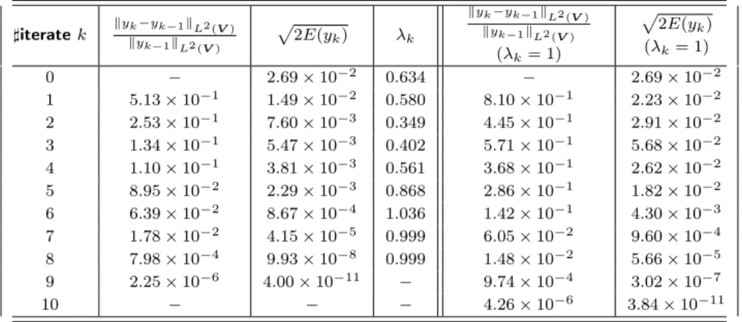
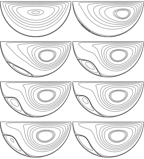
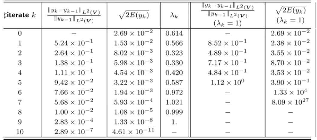
discuss numerical experiments based on finite element approximations in space for two 2D geometries: the celebrated example of the channel with a backward facing step and the semi-circular driven cavity introduced in [6]. We notably exhibit the robustness of the damped Newton method (compared to the Newton one), including for small values of the viscosity constant. Section 5 concludes with some perspectives.
We emphasize that the 3D case can be addressed as well: we refer to [14, 13].
2 Analysis of a Least-squares method for a
steady Navier-Stokes equation
We analyse in this section a least-squares method to solve the steady Navier-Stokes equation (1.4): we follow and improve [11] where the particular case 𝛼 = 0 is addressed.
2.1 Technical preliminary results
We endow the space 𝑉 with the norm ‖𝑦‖𝑉 := ‖∇𝑦‖2, for all 𝑦 ∈ 𝑉 . We shall
also use the following notations
|||𝑦|||2𝑉 := 𝛼‖𝑦‖22+ 𝜈‖∇𝑦‖22, ∀𝑦 ∈ 𝑉
and < 𝑦, 𝑧 >𝑉:= 𝛼 ∫︀
Ω𝑦𝑧 + 𝜈 ∫︀
Ω∇𝑦 · ∇𝑧 so that < 𝑦, 𝑧 >𝑉≤ |||𝑦|||𝑉|||𝑧|||𝑉 for any
𝑦, 𝑧 ∈ 𝑉 .
In the sequel, we repeatedly use the following classical estimates (see [24]). Lemma 2.1. Let any 𝑢, 𝑣 ∈ 𝑉 . Then
− ∫︁ Ω 𝑢 · ∇𝑢 · 𝑣 = ∫︁ Ω 𝑢 · ∇𝑣 · 𝑢 ≤√2‖𝑢‖2‖∇𝑣‖2‖∇𝑢‖2. (2.1)
Definition 2.1. For any 𝑦 ∈ 𝑉 , we define 𝜏 (𝑦) :=√‖𝑦‖𝑉
2𝛼𝜈.
We shall also repeatedly use the following Young type inequalities. Lemma 2.2. For any 𝑢, 𝑣 ∈ 𝑉 , the following inequality holds true :
√
2‖𝑢‖2‖∇𝑣‖2‖∇𝑢‖2≤ 𝜏 (𝑣)|||𝑢|||2𝑉 (2.2)
Let 𝑓 ∈ 𝐻−1(Ω)2, 𝑔 ∈ 𝐿2(Ω)2and 𝛼 ∈R⋆+. The following result holds true:
Proposition 2.3. Assume Ω ⊂R𝑑 is bounded and Lipschitz. There exists at least one solution 𝑦 of (1.4) satisfying
|||𝑦|||2𝑉 ≤ 𝑐0𝜈‖𝑓 ‖2𝐻−1(Ω)𝑑+ 𝛼‖𝑔‖
2
2 (2.3)
where 𝑐0> 0, only connected to the Poincaré constant, depends on Ω. If moreover,
Ω is 𝐶2 and 𝑓 ∈ 𝐿2(Ω)𝑑, then any solution 𝑦 ∈ 𝑉 of (1.4) belongs to 𝐻2(Ω)2. Proof. We refer to [15].
Lemma 2.4. Assume that a solution 𝑦 ∈ 𝑉 of (1.4) satisfies 𝜏 (𝑦) < 1. Then, such solution is the unique solution of (1.4).
Proof. Let 𝑦1∈ 𝑉 and 𝑦2∈ 𝑉 be two solutions of (1.4). Set 𝑌 = 𝑦1− 𝑦2. Then,
𝛼 ∫︁ Ω 𝑌 · 𝑤 + 𝜈 ∫︁ Ω ∇𝑌 · ∇𝑤 + ∫︁ Ω 𝑦2· ∇𝑌 · 𝑤 + ∫︁ Ω 𝑌 · ∇𝑦1· 𝑤 = 0 ∀𝑤 ∈ 𝑉 .
We now take 𝑤 = 𝑌 and use that∫︀
Ω𝑦2· ∇𝑌 · 𝑌 = 0. We use (2.1) and (2.2) to get
|||𝑌 |||2𝑉 = −
∫︁ Ω
𝑌 · ∇𝑦1· 𝑌 ≤ 𝜏 (𝑦1)|||𝑌 |||2𝑉
leading to (1 − 𝜏 (𝑦1))|||𝑌 |||2𝑉 ≤ 0. Consequently, if 𝜏 (𝑦1) < 1 then 𝑌 = 0 and the
solution of (1.4) is unique. In particular, in view of (2.3), this holds if the data satisfy 𝜈‖𝑔‖22+𝑐𝛼0‖𝑓 ‖
2
𝐻−1(Ω)𝑑< 2𝜈
3
.
We now introduce our least-squares functional 𝐸 : 𝑉 →R+ as follows 𝐸(𝑦) :=1 2 ∫︁ Ω (𝛼|𝑣|2+ 𝜈|∇𝑣|2) = 1 2|||𝑣||| 2 𝑉 (2.4)
where the corrector 𝑣 ∈ 𝑉 is the unique solution of the linear formulation (1.9). In particular, the corrector 𝑣 satisfies the estimate:
|||𝑣|||𝑉 ≤ |||𝑦|||𝑉 (︂ 1 +|||𝑦|||𝑉 2√𝛼𝜈 )︂ + √︂ 𝑐0‖𝑓 ‖2𝐻−1 𝜈 + 𝛼‖𝑔‖ 2 2. (2.5)
Conversely, we also have
|||𝑦|||𝑉 ≤ |||𝑣|||𝑉 + √︂ 𝑐0‖𝑓 ‖2𝐻−1 𝜈 + 𝛼‖𝑔‖ 2 2. (2.6)
The infimum of 𝐸 is equal to zero and is reached by a solution of (1.4). In this sense, the functional 𝐸 is a so-called error functional which measures, through the corrector variable 𝑣, the deviation of the pair 𝑦 from being a solution of the underlying equation (1.4).
A practical way of taking a functional to its minimum is through some (clever) use of descent directions, i.e. the use of its derivative. In doing so, the presence of local minima is always something that may dramatically spoil the whole scheme. The unique structural property that discards this possibility is the strict convexity of the functional. However, for non-linear equations like (1.4), one cannot expect this property to hold for the functional 𝐸 in (2.4). Nevertheless, we insist in that for a descent strategy applied to the extremal problem min𝑦∈𝑉𝐸(𝑦) numerical
procedures cannot converge except to a global minimizer leading 𝐸 down to zero. Indeed, we would like to show that the only critical points for 𝐸 correspond to solutions of (1.4). In such a case, the search for an element 𝑦 solution of (1.4) is reduced to the minimization of 𝐸.
For any 𝑦 ∈ 𝑉 , we now look for an element 𝑌1∈ 𝑉 solution of the following
formulation 𝛼 ∫︁ Ω 𝑌1·𝑤+𝜈 ∫︁ Ω ∇𝑌1·∇𝑤+ ∫︁ Ω (𝑦·∇𝑌1+𝑌1·∇𝑦)·𝑤 = −𝛼 ∫︁ Ω 𝑣·𝑤−𝜈 ∫︁ Ω ∇𝑣·∇𝑤, ∀𝑤 ∈ 𝑉 (2.7)
where 𝑣 ∈ 𝑉 is the corrector (associated to 𝑦) solution of (1.9). 𝑌1 enjoys the
following property.
Proposition 2.5. For all 𝑦 ∈ 𝑉 satisfying 𝜏 (𝑦) < 1, there exists a unique solution 𝑌1 of (2.7) associated to 𝑦. Moreover, this solution satisfies
(1 − 𝜏 (𝑦))|||𝑌1|||𝑉 ≤ √︀
2𝐸(𝑦). (2.8)
Proof. The proof uses the arguments of Lemma 2.4. We define the bilinear and continuous form 𝑎 : 𝑉 × 𝑉 →Rby 𝑎(𝑌, 𝑤) = 𝛼 ∫︁ Ω 𝑌 · 𝑤 + 𝜈 ∫︁ Ω ∇𝑌 · ∇𝑤 + ∫︁ Ω (𝑦 · ∇𝑌 + 𝑌 · ∇𝑦) · 𝑤. (2.9) so that 𝑎(𝑌, 𝑌 ) = |||𝑌 |||2𝑉 +∫︀ Ω𝑌 · ∇𝑦 · 𝑌 . Using (2.2), we obtain 𝑎(𝑌, 𝑌 ) ≥
(1 − 𝜏 (𝑦))|||𝑌 |||2𝑉 for all 𝑌 ∈ 𝑉 . Lax-Milgram lemma leads to the existence and uniqueness of 𝑌1provided 𝜏 (𝑦) < 1. Then, putting 𝑤 = 𝑌1 in (2.7) implies
𝑎(𝑌1, 𝑌1) ≤ −𝛼 ∫︁ Ω 𝑣 · 𝑌1− 𝜈 ∫︁ Ω ∇𝑣 · ∇𝑌1≤ |||𝑌1|||𝑉|||𝑣|||𝑉 = |||𝑌1|||𝑉 √︀ 2𝐸(𝑦) leading to (2.8).
We now check the differentiability of the least-squares functional.
Proposition 2.6. For all 𝑦 ∈ 𝑉 , the map 𝑌 ↦→ 𝐸(𝑦 + 𝑌 ) is a differentiable function on the Hilbert space 𝑉 and for any 𝑌 ∈ 𝑉 , we have
𝐸′(𝑦) · 𝑌 =
∫︁ Ω
𝛼 𝑣 · 𝑉 + 𝜈∇𝑣 · ∇𝑉 (2.10)
where 𝑉 ∈ 𝑉 is the unique solution of 𝛼 ∫︁ Ω 𝑉 ·𝑤+𝜈 ∫︁ Ω ∇𝑉 ·∇𝑤 = −𝛼 ∫︁ Ω 𝑌 ·𝑤−𝜈 ∫︁ Ω ∇𝑌 ·∇𝑤− ∫︁ Ω (𝑦·∇𝑌 +𝑌 ·∇𝑦)·𝑤, ∀𝑤 ∈ 𝑉 . (2.11) Proof. Let 𝑦 ∈ 𝑉 and 𝑌 ∈ 𝑉 . We have 𝐸(𝑦 + 𝑌 ) = 12⃒⃒
⃒ ⃒ ⃒ ⃒𝑉 ⃒ ⃒ ⃒ ⃒ ⃒ ⃒ 2 𝑉 where 𝑉 ∈ 𝑉 is the unique solution of 𝛼 ∫︁ Ω 𝑉 · 𝑤 + 𝜈 ∫︁ Ω ∇𝑉 · ∇𝑤 + 𝛼 ∫︁ Ω (𝑦 + 𝑌 ) · 𝑤 + 𝜈 ∫︁ Ω ∇(𝑦 + 𝑌 ) · ∇𝑤 + ∫︁ Ω (𝑦 + 𝑌 ) · ∇(𝑦 + 𝑌 ) · 𝑤 − ⟨𝑓, 𝑤⟩𝑉′×𝑉 − 𝛼 ∫︁ Ω 𝑔𝑤 = 0, ∀𝑤 ∈ 𝑉 .
If 𝑣 ∈ 𝑉 is the solution of (1.9) associated to 𝑦, 𝑣′∈ 𝑉 is the unique solution of 𝛼 ∫︁ Ω 𝑣′· 𝑤 + 𝜈 ∫︁ Ω ∇𝑣′· ∇𝑤 + ∫︁ Ω 𝑌 · ∇𝑌 · 𝑤 = 0, ∀𝑤 ∈ 𝑉 (2.12)
and 𝑉 ∈ 𝑉 is the unique solution of (2.11), then it is straightforward to check that 𝑉 − 𝑣 − 𝑣′− 𝑉 ∈ 𝑉 is solution of 𝛼 ∫︁ Ω (𝑉 − 𝑣 − 𝑣′− 𝑉 ) · 𝑤 + 𝜈 ∫︁ Ω ∇(𝑉 − 𝑣 − 𝑣′− 𝑉 ) · ∇𝑤 = 0, ∀𝑤 ∈ 𝑉
and therefore𝑉 − 𝑣 − 𝑣′− 𝑉 = 0. Thus 𝐸(𝑦 + 𝑌 ) =1 2 ⃒ ⃒ ⃒ ⃒ ⃒ ⃒𝑣 + 𝑣 ′ + 𝑉⃒⃒ ⃒ ⃒ ⃒ ⃒ 2 𝑉 =1 2|||𝑣||| 2 𝑉 + 1 2 ⃒ ⃒ ⃒ ⃒ ⃒ ⃒𝑣′ ⃒ ⃒ ⃒ ⃒ ⃒ ⃒ 2 𝑉 + 1 2|||𝑉 ||| 2 𝑉 + ⟨𝑉, 𝑣 ′⟩ 𝑉 + ⟨𝑉, 𝑣⟩𝑉 + ⟨𝑣, 𝑣′⟩𝑉. (2.13) Then, writing (2.11) with 𝑤 = 𝑉 and using (2.1), we obtain
|||𝑉 |||2𝑉 ≤ |||𝑉 |||𝑉|||𝑌 |||𝑉 +√2(‖𝑦‖2‖∇𝑌 ‖2+ ‖𝑌 ‖2‖∇𝑦‖2)‖∇𝑉 ‖2 ≤ |||𝑉 |||𝑉|||𝑌 |||𝑉 + √ 2 √ 𝛼𝜈|||𝑦|||𝑉|||𝑌 |||𝑉‖∇𝑉 ‖2 leading to |||𝑉 |||𝑉 ≤ |||𝑌 |||𝑉(1 + √ 2 √
𝛼𝜈|||𝑦|||𝑉). Similarly, using (2.12), we obtain ⃒ ⃒ ⃒ ⃒ ⃒ ⃒𝑣′ ⃒ ⃒ ⃒ ⃒ ⃒ ⃒ 𝑉 ≤ 1 √ 2𝛼𝜈|||𝑌 ||| 2 𝑉. It follows that 1 2 ⃒ ⃒ ⃒ ⃒ ⃒ ⃒𝑣′ ⃒ ⃒ ⃒ ⃒ ⃒ ⃒ 2 𝑉+ 1 2|||𝑉 ||| 2 𝑉 + ⟨𝑉, 𝑣 ′⟩ 𝑉+ ⟨𝑣, 𝑣′⟩𝑉 =
𝑜(|||𝑌 |||𝑉) and from (2.13) that
𝐸(𝑦 + 𝑌 ) = 𝐸(𝑦) + ⟨𝑣, 𝑉 ⟩ + 𝑜(|||𝑌 |||𝑉). Eventually, the estimate |⟨𝑣, 𝑉 ⟩𝑉| ≤ |||𝑣|||𝑉|||𝑉 |||𝑉 ≤ (1+
√ 2 √ 𝛼𝜈|||𝑦|||𝑉) √︀ 𝐸(𝑦)|||𝑌 |||𝑉 gives the continuity of the linear map 𝑌 ↦→ ⟨𝑣, 𝑉 ⟩𝑉.
We are now in position to prove the following result which indicates that, in the ball {𝜏𝑑(𝑦) < 1} of 𝑉 , any critical point for 𝐸 is also a zero of 𝐸.
Proposition 2.7. For all 𝑦 ∈ 𝑉 satisfying 𝜏 (𝑦) < 1, (1 − 𝜏 (𝑦))√︀2𝐸(𝑦) ≤ √1
𝜈‖𝐸
′
(𝑦)‖𝑉′.
Proof. For any 𝑌 ∈ 𝑉 , 𝐸′(𝑦) · 𝑌 =∫︀Ω𝛼 𝑣 · 𝑉 + 𝜈∇𝑣 · ∇𝑉 where 𝑉 ∈ 𝑉 is the unique solution of (2.11). In particular, taking 𝑌 = 𝑌1 defined by (2.7), we obtain
an element 𝑉1∈ 𝑉 solution of 𝛼 ∫︁ Ω 𝑉1·𝑤+𝜈 ∫︁ Ω ∇𝑉1·∇𝑤 = −𝛼 ∫︁ Ω 𝑌1·𝑤−𝜈 ∫︁ Ω ∇𝑌1·∇𝑤− ∫︁ Ω (𝑦·∇𝑌1+𝑌1·∇𝑦)·𝑤, ∀𝑤 ∈ 𝑉 . (2.14)
Summing (2.7) and (2.14), we obtain that 𝑣 − 𝑉1∈ 𝑉 solves 𝛼 ∫︁ Ω (𝑣 − 𝑉1)𝑤 + 𝜈 ∫︁ Ω (∇𝑣 − ∇𝑉1) · 𝑤 = 0, ∀𝑤 ∈ 𝑉 .
This implies that 𝑣 and 𝑉1coincide and then that
𝐸′(𝑦) · 𝑌1= ∫︁ Ω 𝛼|𝑣|2+ 𝜈|∇𝑣|2= 2𝐸(𝑦), ∀𝑦 ∈ 𝑉 . (2.15) It follows that 2𝐸(𝑦) = 𝐸′(𝑦) · 𝑌1≤ ‖𝐸′(𝑦)‖𝑉′‖𝑌1‖𝑉 ≤ ‖𝐸′(𝑦)‖𝑉′|||𝑌√1|||𝑉 𝜈 .
Propo-sition 2.5 allows to conclude.
Eventually, we prove the following coercivity type inequality for the error functional 𝐸.
Proposition 2.8. Assume that a solution 𝑦 ∈ 𝑉 of (1.4) satisfies 𝜏 (𝑦) < 1. Then, for all 𝑦 ∈ 𝑉 ,
|||𝑦 − 𝑦|||𝑉 ≤(︀
1 − 𝜏 (𝑦))︀−1√︀2𝐸(𝑦). (2.16) Proof. For any 𝑦 ∈ 𝑉 , let 𝑣 be the corresponding corrector and let 𝑌 = 𝑦 − 𝑦. We have 𝛼 ∫︁ Ω 𝑌 ·𝑤+𝜈 ∫︁ Ω ∇𝑌 ·∇𝑤+ ∫︁ Ω 𝑦·∇𝑌 ·𝑤+ ∫︁ Ω 𝑌 ·∇𝑦·𝑤 = −𝛼 ∫︁ Ω 𝑣·𝑤−𝜈 ∫︁ Ω ∇𝑣·∇𝑤, ∀𝑤 ∈ 𝑉 . (2.17) For 𝑤 = 𝑌 , this equality rewrites
|||𝑌 |||2𝑉 = − ∫︁ Ω 𝑌 · ∇𝑦 · 𝑌 − 𝛼 ∫︁ Ω 𝑣 · 𝑌 − 𝜈 ∫︁ Ω ∇𝑣 · ∇𝑌.
Repeating the arguments of the proof of Proposition 2.5, the results follows. Assuming the existence of a solution of (1.4) in the ball {𝑦 ∈ 𝑉 , 𝜏 (𝑦) < 1}, Proposition 2.7 and Proposition 2.8 imply that any minimizing sequence {𝑦𝑘}(𝑘∈N)
for 𝐸 uniformly in {𝑦 ∈ 𝑉 , 𝜏 (𝑦) ≤ 1} strongly converges to a solution of (1.4). Remark that, from Lemma 2.4, such solution is unique. In the next section, we construct, assuming the parameter 𝛼 large enough, such sequence {𝑦𝑘}(𝑘∈N).
Remark 2.9. In order to simplify notations, we have introduced the corrector variable 𝑣 leading to the functional 𝐸. Instead, we may consider the functional
̃︀ 𝐸 : 𝑉 →R defined by ̃︀ 𝐸(𝑦) :=1 2‖𝛼𝑦 + 𝜈𝐵1(𝑦) + 𝐵(𝑦, 𝑦) − 𝑓 + 𝛼𝑔‖ 2 𝑉′
with 𝐵1 : 𝑉 → 𝐿2(Ω)2 and 𝐵 : 𝑉 × 𝑉 → 𝐿2(Ω)2 defined by (𝐵1(𝑦), 𝑤) :=
(∇𝑦, ∇𝑤)2 and (𝐵(𝑦, 𝑧), 𝑤) := ∫︀
Ω𝑦 · ∇𝑧 · 𝑤 respectively. 𝐸 and 𝐸 are equivalent.̃︀
Precisely, from the definition of 𝑣 (see (1.9)), we deduce that 𝐸(𝑦) =1 2|||𝑣||| 2 𝑉 ≤ 𝑐20 2𝜈2 ⃦ ⃦𝛼𝑦 + 𝜈𝐵1(𝑦) + 𝐵(𝑦, 𝑦) − 𝑓 + 𝛼𝑔 ⃦ ⃦ 2 𝑉′= 𝑐20 𝜈2𝐸(𝑦),̃︀ ∀𝑦 ∈ 𝑉 . Conversely, ⃦ ⃦𝛼𝑦 + 𝜈𝐵1(𝑦) + 𝐵(𝑦, 𝑦) − 𝑓 + 𝛼𝑔 ⃦ ⃦ 𝑉′= sup 𝑤∈𝑉 ,𝑤̸=0 ∫︀ Ω(𝛼𝑣𝑤 + 𝜈∇𝑣 · ∇𝑤) ‖𝑤‖𝑉 ≤|||𝑣|||𝑉 sup 𝑤∈𝑉 ,𝑤̸=0 |||𝑤|||𝑉 ‖𝑤‖𝑉 ≤ √︁ 𝛼𝑐20+ 𝜈|||𝑣|||𝑉
so that𝐸(𝑦) ≤ (𝛼𝑐̃︀ 20+ 𝜈)𝐸(𝑦) for all 𝑦 ∈ 𝑉 .
2.2 A strongly convergent minimizing sequence for 𝐸
-Link with the damped Newton method
We define in this section a sequence converging strongly to a solution of (1.4) for which 𝐸 vanishes. According to Proposition 2.7, it suffices to define a minimizing sequence for 𝐸 included in the ballB= {𝑦 ∈ 𝑉 , 𝜏 (𝑦) < 1}. In this respect, remark that equality (2.15) shows that −𝑌1 given by the solution of (2.7) is a descent
direction for the functional 𝐸. Therefore, we can define at least formally, for any 𝑚 ≥ 1, a minimizing sequence {𝑦𝑘}(𝑘≥0) as follows:
⎧ ⎪ ⎪ ⎨ ⎪ ⎪ ⎩ 𝑦0∈ 𝐻 given, 𝑦𝑘+1= 𝑦𝑘− 𝜆𝑘𝑌1,𝑘, 𝑘 ≥ 0, 𝜆𝑘= argmin𝜆∈[0,𝑚]𝐸(𝑦𝑘− 𝜆𝑌1,𝑘) (2.18)
with 𝑌1,𝑘∈ 𝑉 the solution of the formulation
𝛼 ∫︁ Ω 𝑌1,𝑘· 𝑤 + 𝜈 ∫︁ Ω ∇𝑌1,𝑘· ∇𝑤 + ∫︁ Ω (𝑦𝑘· ∇𝑌1,𝑘+ 𝑌1,𝑘· ∇𝑦𝑘) · 𝑤 = −𝛼 ∫︁ Ω 𝑣𝑘· 𝑤 − 𝜈 ∫︁ Ω ∇𝑣𝑘· ∇𝑤, ∀𝑤 ∈ 𝑉 (2.19)
and 𝑣𝑘∈ 𝑉 the corrector (associated to 𝑦𝑘) solution of (1.9) leading (see (2.15))
to 𝐸′(𝑦𝑘) · 𝑌1,𝑘= 2𝐸(𝑦𝑘).
Remark that from (2.6), the sequence {𝑦𝑘}𝑘>0 is uniformly bounded since
𝑦𝑘 satisfies |||𝑦𝑘|||𝑉 ≤ √︀ 2𝐸(𝑦𝑘) + √︁ 𝑐0 𝜈‖𝑓 ‖ 2
in order to justify the existence of the element 𝑌1,𝑘, 𝑦𝑘 should satisfy 𝜏 (𝑦𝑘) < 1,
i.e. ‖∇𝑦𝑘‖2<
√
2𝛼𝜈. We proceed in two steps: first, assuming that the sequence {𝑦𝑘}(𝑘>0) defined by (2.18) satisfies 𝜏 (𝑦𝑘) ≤ 𝑐1 < 1 for any 𝑘, we show that
𝐸(𝑦𝑘) → 0 and that {𝑦𝑘} converges strongly in 𝑉 to a solution of (1.4). Then, we
determine sufficient conditions on the initial guess 𝑦0∈ 𝑉 in order that 𝜏 (𝑦𝑘) < 1
for all 𝑘 ∈N.
We start with the following lemma which provides the main property of the sequence {𝐸(𝑦𝑘)}(𝑘≥0).
Lemma 2.10. Assume that the sequence {𝑦𝑘}(𝑘≥0) defined by (2.18) satisfy
𝜏 (𝑦𝑘) < 1. Then, for all 𝜆 ∈R, the following estimate holds true
𝐸(𝑦𝑘− 𝜆𝑌1,𝑘) ≤ 𝐸(𝑦𝑘) (︂ |1 − 𝜆| + 𝜆2(1 − 𝜏 (𝑦𝑘)) −2 √ 𝛼𝜈 √︀ 𝐸(𝑦𝑘) )︂2 . (2.20)
Proof. For any real 𝜆 and any 𝑦𝑘, 𝑤𝑘∈ 𝑉 we get the following expansion :
𝐸(𝑦𝑘− 𝜆𝑤𝑘) = 𝐸(𝑦𝑘) − 𝜆 ∫︁ Ω (𝛼𝑣𝑘𝑣𝑘+ 𝜈∇𝑣𝑘· ∇𝑣𝑘) +𝜆 2 2 ∫︁ Ω (𝛼|𝑣𝑘|2+ 𝜈|∇𝑣𝑘|2+ 2(𝛼𝑣𝑘𝑣𝑘+ 𝜈∇𝑣𝑘· ∇𝑣𝑘)) − 𝜆3 ∫︁ Ω 𝛼𝑣𝑘𝑣𝑘+ 𝜈∇𝑣𝑘· ∇𝑣𝑘+ 𝜆4 2 ∫︁ Ω 𝛼|𝑣𝑘|2+ 𝜈|∇𝑣𝑘|2 (2.21) where 𝑣𝑘, 𝑣𝑘∈ 𝑉 and 𝑣𝑘∈ 𝑉 solves respectively
𝛼 ∫︁ Ω 𝑣𝑘· 𝑤 + 𝜈 ∫︁ Ω ∇𝑣𝑘· ∇𝑤 + 𝛼 ∫︁ Ω 𝑦𝑘· 𝑤 + 𝜈 ∫︁ Ω ∇𝑦𝑘· ∇𝑤 + ∫︁ Ω 𝑦𝑘· ∇𝑦𝑘· 𝑤 =< 𝑓, 𝑤 >𝐻−1(Ω)2×𝐻1 0(Ω)2 +𝛼 ∫︁ Ω 𝑔 · 𝑤, ∀𝑤 ∈ 𝑉 , (2.22) 𝛼 ∫︁ Ω 𝑣𝑘· 𝑤 + 𝜈 ∫︁ Ω ∇𝑣𝑘· ∇𝑤 + 𝛼 ∫︁ Ω 𝑤𝑘· 𝑤 + 𝜈 ∫︁ Ω ∇𝑤𝑘· ∇𝑤 + ∫︁ Ω 𝑤𝑘· ∇𝑦𝑘· 𝑤 + 𝑦𝑘· ∇𝑤𝑘· 𝑤 = 0, ∀𝑤 ∈ 𝑉 , (2.23) and 𝛼 ∫︁ Ω 𝑣𝑘· 𝑤 + 𝜈 ∫︁ Ω ∇𝑣𝑘· ∇𝑤 + ∫︁ Ω 𝑤𝑘· ∇𝑤𝑘· 𝑤 = 0, ∀𝑤 ∈ 𝑉 . (2.24)
Since the corrector 𝑣𝑘 associated to 𝑌1,𝑘coincides with the corrector 𝑣𝑘 associated to 𝑦𝑘, expansion (2.21) reduces to 𝐸(𝑦𝑘− 𝜆𝑌1,𝑘) = (1 − 𝜆)2𝐸(𝑦𝑘) + 𝜆2(1 − 𝜆) ∫︁ Ω 𝛼𝑣𝑘𝑣𝑘+ 𝜈∇𝑣𝑘∇𝑣𝑘 +𝜆 4 2 ∫︁ Ω 𝛼|𝑣𝑘|2+ 𝜈|∇𝑣𝑘|2 ≤ (1 − 𝜆)2𝐸(𝑦𝑘) + 𝜆2(1 − 𝜆)|||𝑣𝑘|||𝑉 ⃒ ⃒ ⃒ ⃒ ⃒ ⃒𝑣𝑘 ⃒ ⃒ ⃒ ⃒ ⃒ ⃒ 𝑉 + 𝜆4 2 ⃒ ⃒ ⃒ ⃒ ⃒ ⃒𝑣𝑘 ⃒ ⃒ ⃒ ⃒ ⃒ ⃒ 2 𝑉 ≤ (︂ |1 − 𝜆|√︀𝐸(𝑦𝑘) + 𝜆2 √ 2 ⃒ ⃒ ⃒ ⃒ ⃒ ⃒𝑣𝑘 ⃒ ⃒ ⃒ ⃒ ⃒ ⃒𝑉 )︂2 . (2.25) (2.24) then leads to⃒⃒ ⃒ ⃒ ⃒ ⃒𝑣𝑘 ⃒ ⃒ ⃒ ⃒ ⃒ ⃒ 𝑉 ≤ |||𝑌1,𝑘|||2𝑉 √ 2𝛼𝜈 ≤ √ 2(1−𝜏 (𝑦𝑘))−2 𝐸(𝑦√𝛼𝜈𝑘)and to (2.20).
We are now in position to prove the following convergence result for the sequence {𝐸(𝑦𝑘)}(𝑘≥0).
Proposition 2.11. Let {𝑦𝑘}𝑘≥0 be the sequence defined by (2.18). Assume that
there exists a constant 𝑐1∈ (0, 1) such that 𝜏 (𝑦𝑘) ≤ 𝑐1for all 𝑘. Then 𝐸(𝑦𝑘) → 0
as 𝑘 → ∞. Moreover, there exists 𝑘0 ∈N such that the sequence {𝐸(𝑦𝑘)}(𝑘≥𝑘0)
decays quadratically.
Proof. The inequality 𝜏 (𝑦𝑘) ≤ 𝑐1and (2.20) implies that
𝐸(𝑦𝑘− 𝜆𝑌1,𝑘) ≤ 𝐸(𝑦𝑘) (︂ |1 − 𝜆| + 𝜆2𝑐𝛼,𝜈 √︀ 𝐸(𝑦𝑘) )︂2 , 𝑐𝛼,𝜈 := (1 − 𝑐√ 1)−2 𝛼𝜈 . (2.26) Let us denote the polynomial 𝑝𝑘 by 𝑝𝑘(𝜆) = |1 − 𝜆| + 𝜆2𝑐𝛼,𝜈
√︀
𝐸(𝑦𝑘) for all
𝜆 ∈ [0, 𝑚]. So, we can write
√︀ 𝐸(𝑦𝑘+1) = min 𝜆∈[0,𝑚] √︁ 𝐸(𝑦𝑘− 𝜆𝑌1,𝑘) ≤ min 𝜆∈[0,𝑚]𝑝𝑘(𝜆) √︀ 𝐸(𝑦𝑘). If 𝑐𝛼,𝜈 √︀ 𝐸(𝑦0) < 1 (and thus 𝑐𝛼,𝜈 √︀
𝐸(𝑦𝑘) < 1 for all 𝑘 ∈N) then
𝑝𝑘(𝜆̃︀𝑘) := min 𝜆∈[0,𝑚] 𝑝𝑘(𝜆) ≤ 𝑝𝑘(1) = 𝑐𝛼,𝜈 √︀ 𝐸(𝑦𝑘) and thus 𝑐𝛼,𝜈 √︀ 𝐸(𝑦𝑘+1) ≤ (︀ 𝑐𝛼,𝜈 √︀ 𝐸(𝑦𝑘) )︀2 (2.27) implying that 𝑐𝛼,𝜈√︀𝐸(𝑦𝑘) → 0 as 𝑘 → ∞ with a quadratic rate.
Suppose now that 𝑐𝛼,𝜈 √︀
𝐸(𝑦0) ≥ 1 and denote 𝐼 = {𝑘 ∈N, 𝑐𝛼,𝜈 √︀
𝐸(𝑦𝑘) ≥ 1}.
Let us prove that 𝐼 is a finite subset ofN. For all 𝑘 ∈ 𝐼, since 𝑐𝛼,𝜈√︀𝐸(𝑦𝑘) ≥ 1,
min 𝜆∈[0,𝑚]𝑝𝑘(𝜆) = min𝜆∈[0,1]𝑝𝑘(𝜆) = 𝑝𝑘 (︁ 1 2𝑐𝛼,𝜈 √︀ 𝐸(𝑦𝑘) )︁ = 1 − 1 4𝑐𝛼,𝜈 √︀ 𝐸(𝑦𝑘)
and thus, for all 𝑘 ∈ 𝐼, 𝑐𝛼,𝜈 √︀ 𝐸(𝑦𝑘+1) ≤ (︁ 1 − 1 4𝑐𝛼,𝜈√︀𝐸(𝑦𝑘) )︁ 𝑐𝛼,𝜈 √︀ 𝐸(𝑦𝑘) = 𝑐𝛼,𝜈 √︀ 𝐸(𝑦𝑘) − 1 4. This inequality implies that the sequence {𝑐𝛼,𝜈
√︀
𝐸(𝑦𝑘)}𝑘∈N strictly decreases and
thus, there exists 𝑘0∈N such that for all 𝑘 ≥ 𝑘0, 𝑐𝛼,𝜈 √︀
𝐸(𝑦𝑘) < 1. Thus 𝐼 is a
finite subset ofN. Arguing as in the first case, it follows that 𝑐𝛼,𝜈 √︀
𝐸(𝑦𝑘) → 0 as
𝑘 → ∞.
In both cases, remark that 𝑝𝑘(̃︀𝜆𝑘) decreases with respect to 𝑘.
Lemma 2.12. Assume that the sequence {𝑦𝑘}(𝑘≥0) defined by (2.18) satisfies
𝜏 (𝑦𝑘) ≤ 𝑐1 for all 𝑘 and some 𝑐1∈ (0, 1). Then 𝜆𝑘→ 1 as 𝑘 → ∞.
Proof. In view of (2.25), we have, as long as 𝐸(𝑦𝑘) > 0,
(1 − 𝜆𝑘)2= 𝐸(𝑦𝑘+1) 𝐸(𝑦𝑘) − 𝜆2𝑘(1 − 𝜆𝑘) ⟨𝑣𝑘, 𝑣𝑘⟩𝑉 𝐸(𝑦𝑘) − 𝜆4𝑘 ⃒ ⃒ ⃒ ⃒ ⃒ ⃒𝑣𝑘 ⃒ ⃒ ⃒ ⃒ ⃒ ⃒ 2 𝑉 2𝐸(𝑦𝑘) .
From the proof of lemma 2.10, ⟨𝑣𝑘,𝑣𝑘⟩𝑉
𝐸(𝑦𝑘) ≤ 𝐶(𝛼, 𝜈)(1 − 𝑐1) −2√︀ 𝐸(𝑦𝑘) while |||𝑣𝑘|||2𝑉 𝐸(𝑦𝑘) ≤ 𝐶(𝛼, 𝜈) 2
(1−𝑐1)−4𝐸(𝑦𝑘). Consequently, since 𝜆𝑘∈ [0, 𝑚] and 𝐸(𝑦𝑘+1)
𝐸(𝑦𝑘) →
0, we deduce that (1 − 𝜆𝑘)2→ 0, that is 𝜆𝑘 → 1 as 𝑘 → ∞.
Proposition 2.13. Let {𝑦𝑘} be the sequence defined by (2.18). Assume that there
exists a constant 𝑐1 ∈ (0, 1) such that 𝜏 (𝑦𝑘) ≤ 𝑐1 for all 𝑘. Then, 𝑦𝑘 → 𝑦 in 𝑉
where 𝑦 ∈ 𝑉 is the unique solution of (1.4).
Proof. Remark that we can not use Proposition 2.8 since we do not know yet that there exists a solution, say 𝑧, of (1.4) satisfying 𝜏 (𝑧) < 1. In view of 𝑦𝑘+1=
𝑦0−∑︀𝑘𝑛=0𝜆𝑛𝑌1,𝑛, we write 𝑘 ∑︁ 𝑛=0 |𝜆𝑛| ⃒ ⃒ ⃒ ⃒ ⃒ ⃒𝑌1,𝑛 ⃒ ⃒ ⃒ ⃒ ⃒ ⃒ 𝑉 ≤ 𝑚 𝑘 ∑︁ 𝑛=0 ⃒ ⃒ ⃒ ⃒ ⃒ ⃒𝑌1,𝑛 ⃒ ⃒ ⃒ ⃒ ⃒ ⃒ 𝑉 ≤ 𝑚 √ 2 𝑘 ∑︁ 𝑛=0 √︀ 𝐸(𝑦𝑛) 1 − 𝜏𝑑(𝑦𝑛) ≤ 𝑚√2 1 − 𝑐1 𝑘 ∑︁ 𝑛=0 √︀ 𝐸(𝑦𝑛).
Using that 𝑝𝑛(̃︀𝜆𝑛) ≤ 𝑝0(̃︀𝜆0) for all 𝑛 ≥ 0, we can write for 𝑛 > 0, √︀ 𝐸(𝑦𝑛) ≤ 𝑝𝑛−1(̃︀𝜆𝑛−1) √︀ 𝐸(𝑦𝑛−1) ≤ 𝑝0(̃︀𝜆0) √︀ 𝐸(𝑦𝑛−1) ≤ 𝑝0(̃︀𝜆0)𝑛 √︀ 𝐸(𝑦0), we finally obtain 𝑘 ∑︁ 𝑛=0 |𝜆𝑛|⃒⃒ ⃒ ⃒ ⃒ ⃒𝑌1,𝑛 ⃒ ⃒ ⃒ ⃒ ⃒ ⃒ 𝑉 ≤ 𝑚√2 1 − 𝑐1 √︀ 𝐸(𝑦0) 1 − 𝑝0(̃︀𝜆0)
for which we deduce that the serie∑︀
𝑘≥0𝜆𝑘𝑌1,𝑘converges in 𝑉 . Then, 𝑦𝑘converges
the convergence of the corrector 𝑣𝑘 to 0 in 𝑉 ; taking the limit in the corrector
equation (2.22) shows that 𝑦 solves (1.4). Since 𝜏 (𝑦) ≤ 𝑐1< 1, lemma 2.4 shows
that this solution is unique.
As mentioned earlier, the remaining and crucial point is to show that the sequence {𝑦𝑘} may satisfies the uniform property 𝜏 (𝑦𝑘) ≤ 𝑐1 for some 𝑐1< 1.
Lemma 2.14. Assume that 𝑦0= 𝑔 ∈ 𝑉 . For all 𝑐1∈ (0, 1) there exists 𝛼0> 0,
such that, for any 𝛼 ≥ 𝛼0, the unique sequence defined by (2.18) satisfies 𝜏 (𝑦𝑘) ≤ 𝑐1
for all 𝑘 ≥ 0.
Proof. Let 𝑐1∈ (0, 1) and assume that 𝑦0belongs to 𝑉 . There exists 𝛼1> 0 such
that, for all 𝛼 ≥ 𝛼1, 𝜏 (𝑦0) ≤ 𝑐21.
Moreover, in view of the above computation, for all 𝛼 > 0, since for all 𝑣 ∈ 𝑉 ‖𝑣‖𝑉 ≤ 1𝜈|||𝑣|||𝑉, for all 𝑘 ∈N ‖𝑦𝑘+1‖𝑉 ≤ ‖𝑦0‖𝑉 + 𝑚√2 𝜈(1 − 𝑐1) √︀ 𝐸(𝑦0) 1 − 𝑝0(̃︀𝜆0) where √︀ 𝐸(𝑦0) 1 − 𝑝0(̃︀𝜆0) ≤ ⎧ ⎪ ⎨ ⎪ ⎩ √︀ 𝐸(𝑦0) 1 − 𝑐𝛼,𝜈 √︀ 𝐸(𝑦0) , if 𝑐𝛼,𝜈 √︀ 𝐸(𝑦0) < 1, 4𝑐𝛼,𝜈𝐸(𝑦0), if 𝑐𝛼,𝜈 √︀ 𝐸(𝑦0) ≥ 1.
From (1.9), we obtain that |||𝑣|||2𝑉 ≤ 𝛼‖𝑔 − 𝑦‖22+ 1 𝜈 (︂ 𝜈‖∇𝑦‖2+ ‖𝑦‖2‖∇𝑦‖2+ √ 𝑐0‖𝑓 ‖𝐻−1(Ω)2 )︂2 . In particular, taking 𝑦 = 𝑦0= 𝑔 allows to remove the 𝛼 term in the right hand side
and gives 𝐸(𝑔) ≤ 1 2𝜈 (︁ ‖𝑔‖𝑉(𝜈 + ‖𝑔‖2) + √ 𝑐0‖𝑓 ‖𝐻−1(Ω)2 )︁2 := 1 2𝜈𝑐2(𝑓, 𝑔), (2.28) and thus, if 𝑐𝛼1,𝜈 √︀
𝐸(𝑔) ≥ 1, then for all 𝛼 ≥ 𝛼1 such that 𝑐𝛼,𝜈√︀𝐸(𝑔) ≥ 1 and
for all 𝑘 ∈N: ‖𝑦𝑘+1‖𝑉 ≤ ‖𝑔‖𝑉 + 𝑚√2 𝜈(1 − 𝑐1) √︀ 𝐸(𝑔) 1 − 𝑝0(̃︀𝜆0) ≤ ‖𝑔‖𝑉 + 2𝑚√2 𝜈3√𝛼(1 − 𝑐 1)3 𝑐2(𝑓, 𝑔). (2.29) If now 𝑐𝛼1,𝜈 √︀
𝐸(𝑔) < 1 then there exists 0 < 𝐾 < 1 such that for all 𝛼 ≥ 𝛼1
we have 𝑐𝛼,𝜈 √︀
𝐸(𝑔) ≤ 𝐾. We therefore have for all 𝛼 ≥ 𝛼1 √︀ 𝐸(𝑔) 1 − 𝑝0(̃︀𝜆0) ≤ √︀ 𝐸(𝑔) 1 − 𝐾
and thus for all 𝑘 ∈N: ‖𝑦𝑘+1‖𝑉 ≤ ‖𝑔‖𝑉+ 𝑚√2 𝜈(1 − 𝑐1) √︀ 𝐸(𝑔) 1 − 𝑝0(̃︀𝜆0) ≤ ‖𝑔‖𝑉+ 𝑚 𝜈3/2(1 − 𝑐 1)(1 − 𝐾) √︀ 𝑐2(𝑓, 𝑔). (2.30) On the other hand, there exists 𝛼0≥ 𝛼1 such that, for all 𝛼 ≥ 𝛼0we have
2𝑚√2 𝜈3√𝛼(1 − 𝑐 1)3 𝑐2(𝑓, 𝑔) ≤ 𝑐1 2 √ 2𝛼𝜈 and 𝑚 𝜈3/2(1 − 𝑐 1)(1 − 𝐾) √︀ 𝑐2(𝑓, 𝑔) ≤ 𝑐1 2 √ 2𝛼𝜈.
We then deduce from (2.29) and (2.30) that for all 𝛼 ≥ 𝛼0and for all 𝑘 ∈N: ‖𝑦𝑘+1‖𝑉 ≤ 𝑐1 2 √ 2𝛼𝜈 + 𝑐1 2 √ 2𝛼𝜈 = 𝑐1 √ 2𝛼𝜈 that is 𝜏 (𝑦𝑘+1) ≤ 𝑐1.
Gathering the previous lemmas and propositions, we can now deduce the strong convergence of the sequence {𝑦𝑘}𝑘≥0 defined by (2.18), initialized by 𝑦0= 𝑔.
Theorem 2.15. Let 𝑐1 ∈ (0, 1). Assume that 𝑦0= 𝑔 ∈ 𝑉 and 𝛼 is large enough
so that 𝑐2(𝑓, 𝑔) ≤ max (︁1 − 𝑐1 2 , 𝑐1 √ 𝜈(1 − 𝐾2) 𝑚 )︁𝑐1 4𝑚𝜈 5/2 (1 − 𝑐1)22𝛼𝜈 (2.31)
Then, the sequence {𝑦𝑘}(𝑘∈N) defined by (2.18) strongly converges to the unique
solution 𝑦 of (1.4). Moreover, there exists 𝑘0∈Nsuch that the sequence {𝑦𝑘}𝑘≥𝑘0
converges quadratically to 𝑦. Moreover, this solution satisfies 𝜏 (𝑦) < 1.
2.3 Remarks
The following remarks are in order.
Remark 2.16. Estimate (2.3) is usually used to obtain a sufficient condition on the data 𝑓, 𝑔 to ensure the uniqueness of the solution of (1.4) (i.e. 𝜏 (𝑦) < 1): it leads to
𝛼‖𝑔‖22+ 𝑐0𝜈‖𝑓 ‖2(𝐻−1(Ω))2 ≤ 2𝛼𝜈2, if 𝑑 = 2, (2.32)
We emphasize that such (sufficient) conditions are more restrictive than (2.31), as they impose smallness properties on 𝑔: precisely ‖𝑔‖22 ≤ 2𝜈2. In particular, this
Remark 2.17. It seems surprising that the algorithm (2.18) achieves a quadratic rate for 𝑘 large. Let us consider the application ℱ : 𝑉 → 𝑉′ defined as ℱ (𝑦) = 𝛼𝑦 + 𝜈𝐵1(𝑦) + 𝐵(𝑦, 𝑦) − 𝑓 − 𝛼𝑔. The sequence {𝑦𝑘}𝑘>0 associated to the Newton
method to find the zero of 𝐹 is defined as follows:
{︃
𝑦0∈ 𝑉 ,
ℱ′(𝑦𝑘) · (𝑦𝑘+1− 𝑦𝑘) = −ℱ (𝑦𝑘), 𝑘 ≥ 0.
(2.33)
We check that this sequence coincides with the sequence obtained from (2.18) if 𝜆𝑘 is fixed equal to one and if 𝑦0 ∈ 𝑉 . The algorithm (2.18) which consists to
optimize the parameter 𝜆𝑘 ∈ [0, 𝑚], 𝑚 ≥ 1, in order to minimize 𝐸(𝑦𝑘),
equiv-alently ‖ℱ (𝑦𝑘)‖𝑉′, corresponds to the so-called in the literature damped Newton
method for the application ℱ (see [4]). As the iterates increase, the optimal pa-rameter 𝜆𝑘 converges to one (according to Lemma 2.12), this globally convergent
method behaves like the standard Newton method (for which 𝜆𝑘 is fixed equal to
one): this explains the quadratic rate after a finite number of iterates. To the best of our knowledge, this is the first analysis of the damped Newton method for a par-tiel differential equation. Among the few numerical works devoted to the damped Newton method for partial differential equations, we mention [20] for computing viscoplastic fluid flows.
Remark 2.18. Section 6, chapter 6 of the book [5] introduces a least-squares method in order to solve an Oseen type equation (without incompressibility con-straint). The convergence of any minimizing sequence toward a solution 𝑦 is proved under the a priori assumption that the operator 𝐷𝐹 (𝑦) defined as follows
𝐷𝐹 (𝑦) · 𝑤 = 𝛼 𝑤 − 𝜈Δ𝑤 + [(𝑤 · ∇)𝑦 + (𝑦 · ∇)𝑤], ∀𝑤 ∈ 𝑉 (2.34) (for some 𝛼 > 0) is an isomorphism from 𝑉 onto 𝑉′. 𝑦 is then said to be a nonsingular point. According to Proposition 2.5, a sufficient condition for 𝑦 to be a nonsingular point is 𝜏 (𝑦) < 1. Recall that 𝜏 depends on 𝛼. As far as we know, determining a weaker condition ensuring that 𝐷𝐹 (𝑦) is an isomorphism is an open question. Moreover, according to Lemma 2.4, it turns out that this condition is also a sufficient condition for the uniqueness of (1.4). Theorem 2.15 asserts that, if 𝛼 is large enough, then the sequence {𝑦𝑘}(𝑘∈N)defined in (2.18), initialized with 𝑦0= 𝑔,
is a convergent sequence of nonsingular points. Since 𝜆𝑘 is constant equal to one,
this shows the convergence of the Newton method to solve the steady Navier-Stokes equation.
Remark 2.19. We may also define a minimizing sequence for 𝐸 using the gradi-ent 𝐸′: ⎧ ⎪ ⎪ ⎨ ⎪ ⎪ ⎩ 𝑦0∈ 𝐻 given, 𝑦𝑘+1= 𝑦𝑘− 𝜆𝑘𝑔𝑘, 𝑘 ≥ 0, 𝜆𝑘= argmin𝜆∈[0,𝑚]𝐸(𝑦𝑘− 𝜆𝑔𝑘) (2.35)
with 𝑔𝑘 ∈ 𝑉 such that (𝑔𝑘, 𝑤)𝑉 = (𝐸′(𝑦𝑘), 𝑤)𝑉′,𝑉 for all 𝑤 ∈ 𝑉 . In particular,
‖𝑔𝑘‖𝑉 = ‖𝐸′(𝑦𝑘)‖𝑉′. Using the expansion (2.13) with 𝑤𝑘= 𝑔𝑘, we can prove the
linear decrease of the sequence {𝐸(𝑦𝑘)}𝑘>0 to zero assuming however that 𝐸(𝑦0)
is small enough, of the order of 𝜈2, independently of the value of 𝛼.
2.4 Application to the backward Euler scheme
We use the analysis of the previous section to discuss the resolution of the backward Euler scheme (1.3) through a least-squares method. The weak formulation of this scheme reads as follows: given 𝑦0= 𝑢0∈ 𝐻, the sequence {𝑦𝑛}𝑛>0in 𝑉 is defined
by recurrence as follows: ∫︁ Ω 𝑦𝑛+1− 𝑦𝑛 𝛿𝑡 ·𝑤+𝜈 ∫︁ Ω ∇𝑦𝑛+1·∇𝑤+ ∫︁ Ω 𝑦𝑛+1·∇𝑦𝑛+1·𝑤 =< 𝑓𝑛, 𝑤 >𝐻−1(Ω)𝑑×𝐻1 0(Ω)𝑑 (2.36) with 𝑓𝑛defined by (1.5) in term of the external force of the Navier-Stokes model (1.1). We recall that a piecewise linear interpolation in time of {𝑦𝑛}𝑛≥0 weakly
converges in 𝐿2(0, 𝑇, 𝑉 ) toward a solution of (1.2)
As done in [2], one may use the least-squares method (analyzed in Section 2) to solve iteratively (2.36). Precisely, in order to approximate 𝑦𝑛+1from 𝑦𝑛, one may consider the following extremal problem
inf 𝑦∈𝑉𝐸𝑛(𝑦), 𝐸𝑛(𝑦) = 1 2|||𝑣||| 2 𝑉 (2.37)
where the corrector 𝑣 ∈ 𝑉 solves 𝛼 ∫︁ Ω 𝑣 · 𝑤 + 𝜈 ∫︁ Ω ∇𝑣 · ∇𝑤 = −𝛼 ∫︁ Ω 𝑦 · 𝑤 − 𝜈 ∫︁ Ω ∇𝑦 · ∇𝑤 − ∫︁ Ω 𝑦 · ∇𝑦 · 𝑤 + < 𝑓𝑛, 𝑤 >𝐻−1(Ω)2×𝐻1 0(Ω)2+𝛼 ∫︁ Ω 𝑦𝑛· 𝑤, ∀𝑤 ∈ 𝑉 (2.38)
with 𝛼 and 𝑓𝑛 given by (1.5). For any 𝑛 ≥ 0, a minimizing sequence {𝑦𝑛𝑘}(𝑘≥0) for 𝐸𝑛 is defined as follows : ⎧ ⎪ ⎪ ⎨ ⎪ ⎪ ⎩ 𝑦𝑛+10 = 𝑦𝑛, 𝑦𝑛+1𝑘+1= 𝑦𝑛+1𝑘 − 𝜆𝑘𝑌 𝑛+1 1,𝑘 , 𝑘 ≥ 0, 𝜆𝑘= argmin𝜆∈[0,𝑚]𝐸𝑛(𝑦𝑛𝑘− 𝜆𝑌 𝑛 1,𝑘) (2.39)
where 𝑌1,𝑘𝑛 ∈ 𝑉 solves (2.19). Remark that, in view of Theorem 2.15, the first element of the minimizing sequence is chosen equal to 𝑦𝑛, i.e. the minimizer of 𝐸𝑛−1.
The main goal of this section is to prove that for all 𝑛 ∈N, the minimizing sequence (𝑦𝑘𝑛+1)𝑘∈Ndo converges to a solution 𝑦𝑛+1of (2.36). This allows to justify the use of least-squares method to solve the backward Euler scheme. Arguing as in Lemma 2.14, we have to prove the existence of a constant 𝑐1∈ (0, 1), such that
𝜏 (𝑦𝑘𝑛) ≤ 𝑐1for all 𝑛 and 𝑘 inN. Remark that the initialization 𝑦𝑛+10 is fixed as the minimizer of the functional 𝐸𝑛−1, obtained at the previous iterate. Consequently, the uniform property 𝜏 (𝑦𝑘𝑛) ≤ 𝑐1is related to the initial guess 𝑦00equal to the initial
position 𝑢0, to the external force 𝑓 (see (1.2)) and to the value of 𝛼. 𝑢0and 𝑓 are
given a priori, On the other hand, the parameter 𝛼, related to the discretization parameter 𝛿𝑡, can be chosen as large as necessary. As we shall see, this uniform property, which is essential to set up the least-squares procedure, requires smallness properties on 𝑢0and 𝑓 .
We start with the following result analogue to Proposition 2.3.
Proposition 2.20. Let (𝑓𝑛)𝑛∈Nbe a sequence in 𝐻−1(Ω)2, 𝛼 > 0 and 𝑦0= 𝑢0∈
𝐻. For any 𝑛 ∈N, there exists a solution 𝑦𝑛+1∈ 𝑉 of 𝛼 ∫︁ Ω (𝑦𝑛+1−𝑦𝑛)·𝑤+𝜈 ∫︁ Ω ∇𝑦𝑛+1·∇𝑤+ ∫︁ Ω 𝑦𝑛+1·∇𝑦𝑛+1·𝑤 =< 𝑓𝑛, 𝑤 >𝐻−1(Ω)2×𝐻1 0(Ω)2 (2.40) for all 𝑤 ∈ 𝑉 . Moreover, for all 𝑛 ∈N, 𝑦𝑛+1satisfies
⃒ ⃒ ⃒ ⃒ ⃒ ⃒ ⃒ ⃒ ⃒𝑦 𝑛+1⃒⃒ ⃒ ⃒ ⃒ ⃒ ⃒ ⃒ ⃒ 2 𝑉 ≤ 𝑐0 𝜈‖𝑓 𝑛 ‖2𝐻−1(Ω)2+ 𝛼‖𝑦𝑛‖22 (2.41)
where 𝑐0 > 0, only connected to the Poincaré constant, depends on Ω. Moreover,
for all 𝑛 ∈N⋆: ‖𝑦𝑛‖22+ 𝜈 𝛼 𝑛 ∑︁ 𝑘=1 ‖∇𝑦𝑘‖22≤ 1 𝜈 (︁𝑐0 𝛼 𝑛−1 ∑︁ 𝑘=0 ‖𝑓𝑘‖2𝐻−1(Ω)2+ 𝜈‖𝑢0‖22 )︁ . (2.42)
Proof. The existence of 𝑦𝑛+1 is given in Proposition 2.3. (2.42) is obtained by summing (2.41).
Remark 2.21. Arguing as in Lemma 2.4, if there exists a solution 𝑦𝑛+1in 𝑉 of (2.38) satisfying 𝜏 (𝑦𝑛+1) < 1, then such solution is unique. In view of Proposition 2.20, this holds true if notably the quantity ℳ(𝑓, 𝛼, 𝜈) defined as follows
ℳ(𝑓, 𝛼, 𝜈) = 1 𝜈2 (︂ 𝑐0 𝛼 𝑛−1 ∑︁ 𝑘=0 ‖𝑓𝑘‖2𝐻−1(Ω)2+ 𝜈‖𝑢0‖22 )︂ (2.43) is small enough.
2.4.1 Uniform convergence of the least-squares method w.r.t. 𝑛 We have the following convergence for weak solutions of (2.40).
Theorem 2.22. Suppose 𝑓 ∈ 𝐿2(0, 𝑇 ; 𝐻−1(Ω)2), 𝑢0 ∈ 𝑉 and let 𝑐(𝑢0, 𝑓 ) be
defined as follows : 𝑐(𝑢0, 𝑓 ) := max (︁1 𝛼‖𝑢0‖ 2 𝑉(𝜈 + ‖𝑢0‖2)2+𝑐0‖𝑓 ‖2𝐿2(0,𝑇 ;𝐻−1(Ω)2), 2𝑐0‖𝑓 ‖2𝐿2(0,𝑇 ;𝐻−1(Ω)2)+ 𝜈‖𝑢0‖22 )︁ . Let 𝛼 large enough and 𝑓𝑛 be given (1.5) by all 𝑛 ∈ {0, · · · , 𝑁 − 1} and let {𝑦𝑛}𝑛∈Nin 𝑉 solution of (2.40). If there exists a constant 𝑐 > 0 such that
𝑐(𝑢0, 𝑓 ) ≤ 𝑐𝜈4 (2.44)
then, for any 𝑛 ≥ 0, the minimizing sequence {𝑦𝑛+1𝑘 }𝑘∈Ndefined by (2.39) strongly converges to the unique of solution of (2.40).
Proof. According to Proposition 2.13, we have to prove the existence of a constant 𝑐1∈ (0, 1) such that, for all 𝑛 ∈ {0, · · · , 𝑁 − 1} and all 𝑘 ∈N, 𝜏 (𝑦𝑛𝑘) ≤ 𝑐1.
For 𝑛 = 0, as in the previous section, it suffices to takes 𝛼 large enough to ensure the conditions (2.31) with 𝑔 = 𝑦00= 𝑢0leading to the property 𝜏 (𝑦0𝑘) < 𝑐1
for all 𝑘 ∈Nand therefore 𝜏 (𝑦1) < 𝑐1.
For the next minimizing sequences, let us recall (see Lemma 2.14) that for all 𝑛 ∈ {0, · · · , 𝑁 − 1} and all 𝑘 ∈N ‖𝑦𝑛+1𝑘 ‖𝑉 ≤ ‖𝑦𝑛‖𝑉 + 𝑚√2 𝜈(1 − 𝑐1) √︀ 𝐸𝑛(𝑦𝑛) 1 − 𝑝𝑛,0(̃︀𝜆𝑛,0)
First, since for all 𝑛 ∈ {0, · · · , 𝑁 − 1}, ‖𝑓𝑛‖2 𝐻−1(Ω)2 ≤ 𝛼‖𝑓 ‖2𝐿2(0,𝑇 ;𝐻−1(Ω)2), we can write 𝐸0(𝑦0) = 𝐸0(𝑢0) ≤ 1 2𝜈 (︁ ‖𝑢0‖𝑉(𝜈 + ‖𝑢0‖2) + √ 𝑐0‖𝑓0‖𝐻−1(Ω)2 )︁2 ≤ 1 𝜈 (︁ ‖𝑢0‖2𝑉(𝜈 + ‖𝑢0‖2)2+ 𝑐0‖𝑢0‖2𝐻−1(Ω)2 )︁ ≤ 𝛼 𝜈 (︁1 𝛼‖𝑢0‖ 2 𝑉(𝜈 + ‖𝑢0‖2)2+ 𝑐0‖𝑓 ‖2𝐿2(0,𝑇 ;𝐻−1(Ω)2) )︁ . Since 𝑦𝑛is solution of (2.40), it follows from (2.38), that for all 𝑛 ∈ {1, · · · , 𝑁 − 1}:
𝐸𝑛(𝑦𝑛) ≤ 𝑐0 2𝜈‖𝑓 𝑛 − 𝑓𝑛−1‖2𝐻−1(Ω)2+ 𝛼 2‖𝑦 𝑛 − 𝑦𝑛−1‖22 ≤ 𝛼 𝜈 (︁ 2𝑐0‖𝑓 ‖2𝐿2(0,𝑇 ;𝐻−1(Ω)2)+ 𝜈‖𝑢0‖22 )︁ . Therefore, for all 𝑛 ∈ {0, · · · , 𝑁 − 1}, 𝐸𝑛(𝑦𝑛) ≤𝛼𝜈𝑐(𝑢0, 𝑓 ).
Let 𝑐1∈ (0, 1) and suppose that 𝑐(𝑢0, 𝑓 ) < (1−𝑐1)4𝜈3. Then, for any 𝐾 ∈ (0, 1),
there exists 𝛼0> 0 such that, for all 𝛼 ≥ 𝛼0𝑐𝛼,𝜈 √︀
𝐸𝑛(𝑦𝑛) ≤ 𝐾 < 1. We therefore
have (see Lemma 2.14), for all 𝛼 ≥ 𝛼0, all 𝑛 ∈ {0, · · · , 𝑁 − 1} and all 𝑘 ∈N:
‖𝑦𝑘𝑛+1‖𝑉 ≤ ‖𝑦𝑛‖𝑉 + 𝑚√2 𝜈(1 − 𝑐1) √︀ 𝐸𝑛(𝑦𝑛) 1 − 𝑐𝛼,𝜈√︀𝐸𝑛(𝑦𝑛) ≤ ‖𝑦𝑛‖𝑉 + 𝑚√2 𝜈(1 − 𝑐1) √︀ 𝐸𝑛(𝑦𝑛) 1 − 𝐾 ≤ ‖𝑦𝑛‖𝑉 + 𝑚√2𝛼 𝜈3/2(1 − 𝑐 1)(1 − 𝐾) √︀ 𝑐(𝑢0, 𝑓 ). (2.45)
From (2.42) we then obtain, for all 𝑛 ∈ {0, · · · , 𝑁 − 1},
‖𝑦𝑛‖𝑉 ≤ √ 𝛼 𝜈 ⎯ ⎸ ⎸ ⎷ 𝑐0 𝛼 𝑛−1 ∑︁ 𝑘=0 ‖𝑓𝑘‖2 𝐻−1(Ω)2+ 𝜈‖𝑢0‖22 and since 𝑐0 𝛼 ∑︀𝑛−1 𝑘=0‖𝑓 𝑘‖2 𝐻−1(Ω)2 ≤ 𝑐0‖𝑓 ‖2𝐿2(0,𝑇 ;𝐻−1(Ω)2), we deduce that if 𝑐0‖𝑓 ‖2𝐿2(0,𝑇 ;𝐻−1(Ω)2)+ 𝜈‖𝑢0‖22≤ 𝑐21 2𝜈 3 then ‖𝑦𝑛‖𝑉 ≤ 𝑐21 √ 2𝛼𝜈. Moreover, assuming 𝑐(𝑢0, 𝑓 ) ≤ 𝑐2 1(1−𝑐1)2(1−𝐾)2 4𝑚 𝜈 4 , we deduce from (2.45), for all 𝑛 ∈ {0, · · · , 𝑁 − 1} and for all 𝑘 ∈N:
‖𝑦𝑘𝑛‖𝑉 ≤ 𝑐1 2 √ 2𝛼𝜈 +𝑐1 2 √ 2𝛼𝜈 = 𝑐1 √ 2𝛼𝜈 that is 𝜏 (𝑦𝑘𝑛) ≤ 𝑐1. The result follow from Proposition 2.13.
We emphasize that, for each 𝑛 ∈N, the limit 𝑦𝑛+1 of the sequence {𝑦𝑛+1𝑘 }𝑘∈N satisfies 𝜏 (𝑦𝑛+1) < 1 and is therefore the unique solution of (2.40). Moreover, for 𝛼 large enough, the condition (2.44) reads as the following smallness property on the data 𝑢0 and 𝑓 : 𝑐0‖𝑓 ‖2𝐿2(0,𝑇 ;𝐻−1(Ω)2)+ 𝜈‖𝑢0‖22 ≤ 𝑐𝜈4. In contrast with the
static case of Section (2) where the unique condition (2.31) on the data 𝑔 is fulfilled as soon as 𝛼 is large, the iterated case requires a condition on the data 𝑢0 and
𝑓 , whatever be the amplitude of 𝛼. Again, this smallness property is introduced in order to guarantees the condition 𝜏 (𝑦𝑛) < 1 for all 𝑛. In view of (2.42), this condition implies notably that ‖𝑦𝑛‖2≤ 𝑐 𝜈3/2 for all 𝑛 > 0.
For regular solutions of (2.40) which we now consider, we may slightly improve the results, notably based on the control of two consecutive elements of the corresponding sequel {𝑦𝑛}𝑛∈N for the 𝐿2norm. We first start with the following result of regularity.
Proposition 2.23. Assume that Ω is 𝐶2, that (𝑓𝑛)𝑛is a sequence in 𝐿2(Ω)2and
that 𝑢0 ∈ 𝑉 . Then, for all 𝑛 ∈ N, any solution 𝑦𝑛+1 ∈ 𝑉 of (2.40) belongs to 𝐻2(Ω)2.
If moreover, there exists 𝐶 > 0 such that 𝑐0 𝛼 𝑛 ∑︁ 𝑘=0 ‖𝑓𝑘‖2𝐻−1(Ω)2+ 𝜈‖𝑦 0 ‖22< 𝐶𝜈3, (2.46) then 𝑦𝑛+1 satisfies ∫︁ Ω |∇𝑦𝑛+1|2+ 𝜈 2𝛼 𝑛+1 ∑︁ 𝑘=1 ∫︁ Ω |𝑃 Δ𝑦𝑘|2≤ 1 𝜈 (︁1 𝛼 𝑛 ∑︁ 𝑘=0 ‖𝑓𝑘‖22+ 𝜈‖∇𝑢0‖22 )︁ (2.47)
where 𝑃 is the operator of projection from 𝐿2(Ω)𝑑 into 𝐻.
Proof. From Proposition 2.3, we know that for all 𝑛 ∈ N*, 𝑦𝑛 ∈ 𝐻2(Ω)2∩ 𝑉 . Taking 𝑤 = 𝑃 Δ𝑦𝑛+1in (2.40) leads to : 𝛼 ∫︁ Ω |∇𝑦𝑛+1|2+ 𝜈 ∫︁ Ω |𝑃 Δ𝑦𝑛+1|2= − ∫︁ Ω 𝑓𝑛𝑃 Δ𝑦𝑛+1+ ∫︁ Ω 𝑦𝑛+1· ∇𝑦𝑛+1· 𝑃 Δ𝑦𝑛+1 + 𝛼 ∫︁ Ω ∇𝑦𝑛· ∇𝑦𝑛+1. (2.48) Recall that ∫︁ Ω 𝑓𝑛𝑃 Δ𝑦𝑛+1≤ 1 2𝜈‖𝑓 𝑛 ‖22+ 𝜈 2‖𝑃 Δ𝑦 𝑛+1 ‖22, 𝛼 ∫︁ Ω ∇𝑦𝑛·∇𝑦𝑛+1≤ 𝛼 2‖𝑦 𝑛 ‖2𝑉+ 𝛼 2‖𝑦 𝑛+1 ‖2𝑉.
We also have ⃒ ⃒ ⃒ ∫︁ Ω 𝑦𝑛+1· ∇𝑦𝑛+1· 𝑃 Δ𝑦𝑛+1⃒⃒ ⃒≤ ‖𝑦 𝑛+1‖ ∞‖∇𝑦𝑛+1‖2‖𝑃 Δ𝑦𝑛+1‖2.
We now use (see [23, chapter 5]) that there exist three constants 𝑐1, 𝑐2and 𝑐3 such
that ‖Δ𝑦𝑛+1‖2≤ 𝑐1‖𝑃 Δ𝑦𝑛+1‖2, ‖𝑦𝑛+1‖∞≤ 𝑐2‖𝑦𝑛+1‖ 1 2 2‖Δ𝑦 𝑛+1 ‖ 1 2 2 and ‖∇𝑦𝑛+1‖2≤ 𝑐3‖𝑦𝑛+1‖ 1 2 2‖Δ𝑦 𝑛+1 ‖12 2.
This implies that (for 𝑐 = 𝑐1𝑐2𝑐3) ⃒ ⃒ ⃒ ∫︁ Ω 𝑦𝑛+1· ∇𝑦𝑛+1· 𝑃 Δ𝑦𝑛+1 ⃒ ⃒ ⃒≤ 𝑐‖𝑦 𝑛+1 ‖2‖𝑃 Δ𝑦𝑛+1‖22.
Recalling (2.48), it follows that 𝛼 2 ∫︁ Ω |∇𝑦𝑛+1|2+ (︂ 𝜈 2− 𝑐‖𝑦 𝑛+1 ‖2 )︂ ∫︁ Ω |𝑃 Δ𝑦𝑛+1|2≤ 1 2𝜈‖𝑓 𝑛 ‖22+ 𝛼 2 ∫︁ Ω |∇𝑦𝑛|2.
But, from estimate (2.42), the assumption (2.46) implies that ‖𝑦𝑛+1‖2≤4𝑐𝜈 and ∫︁ Ω |∇𝑦𝑛+1|2+ 𝜈 2𝛼 ∫︁ Ω |𝑃 Δ𝑦𝑛+1|2≤ 1 𝜈𝛼‖𝑓 𝑛 ‖22+ ∫︁ Ω |∇𝑦𝑛|2.
Summing then implies (2.47) for all 𝑛 ∈N.
Remark 2.24. Under the hypothesis of Proposition 2.23, suppose that
𝐵𝛼,𝜈 := (𝛼𝜈5)−1 (︂ 𝑐0𝛼−1 𝑛 ∑︁ 𝑘=0 ‖𝑓𝑘‖2𝐻−1(Ω)2+𝜈‖𝑦0‖22 )︂(︂ 𝛼−1 𝑛−1 ∑︁ 𝑘=0 ‖𝑓𝑘‖22+𝜈‖∇𝑦0‖22 )︂
is small (which is satisfied as soon as 𝛼 is large enough). Then, the solution of (2.40) is unique.
Indeed, let 𝑛 ∈ N and let 𝑦1𝑛+1, 𝑦𝑛+12 ∈ 𝑉 be two solutions of (2.40). Then 𝑌 := 𝑦𝑛+11 − 𝑦2𝑛+1satisfies 𝛼 ∫︁ Ω 𝑌 · 𝑤 + 𝜈 ∫︁ Ω ∇𝑌 · ∇𝑤 + ∫︁ Ω 𝑦2𝑛+1· ∇𝑌 · 𝑤 + ∫︁ Ω 𝑌 · ∇𝑦𝑛+11 · 𝑤 = 0 ∀𝑤 ∈ 𝑉
and in particular, for 𝑤 = 𝑌 (since∫︀ Ω𝑦 𝑛+1 2 · ∇𝑌 · 𝑌 = 0) 𝛼 ∫︁ Ω |𝑌 |2+ 𝜈 ∫︁ Ω |∇𝑌 |2= − ∫︁ Ω 𝑌 · ∇𝑦1𝑛+1· 𝑌 = ∫︁ Ω 𝑌 · ∇𝑌 · 𝑦𝑛+11 ≤ 𝑐‖𝑦𝑛+11 ‖∞‖∇𝑌 ‖2‖𝑌 ‖2 ≤ 𝑐‖𝑦𝑛+11 ‖ 1/2 2 ‖𝑃 Δ𝑦 𝑛+1 1 ‖ 1/2 2 ‖∇𝑌 ‖2‖𝑌 ‖2 ≤ 𝛼‖𝑌 ‖22+ 𝑐 𝛼‖𝑦 𝑛+1 1 ‖2‖𝑃 Δ𝑦𝑛+11 ‖2‖∇𝑌 ‖22 leading to (︂ 𝜈 − 𝑐 𝛼‖𝑦 𝑛+1 1 ‖2‖𝑃 Δ𝑦1𝑛+1‖2 )︂ ‖∇𝑌 ‖22≤ 0. If ‖𝑦𝑛+11 ‖2‖𝑃 Δ𝑦𝑛+11 ‖2< 𝜈𝛼 𝑐 , (2.49)
then 𝑌 = 0 and the solution is unique. But, from (2.42) and (2.47), ‖𝑦1𝑛+1‖ 2 2‖𝑃 Δ𝑦𝑛+11 ‖ 2 2≤ 4𝛼 𝜈3 (︂ 𝑐0 𝛼 𝑛 ∑︁ 𝑘=0 ‖𝑓𝑘‖2𝐻−1(Ω)2+𝜈‖𝑦0‖22 )︂(︂ 1 𝛼 𝑛 ∑︁ 𝑘=0 ‖𝑓𝑘‖22+𝜈‖∇𝑦0‖22 )︂ . Therefore, if there exists a constant 𝐶 such that 𝐵𝛼,𝜈< 𝐶, then (2.49) holds true.
Proposition 2.23 then allows to obtain the following estimate of ‖𝑦𝑛+1− 𝑦𝑛‖2in
term of the parameter 𝛼.
Theorem 2.25. We assume that Ω is 𝐶2, that (𝑓𝑛)𝑛 is a sequence in 𝐿2(Ω)2
satisfies 𝛼−1∑︀+∞𝑘=0‖𝑓𝑘‖22 < +∞, that 𝑢0 ∈ 𝑉 and that for all 𝑛 ∈N, 𝑦𝑛+1 ∈
𝐻2(Ω)2∩ 𝑉 is a solution of (2.40) satisfying ‖𝑦𝑛+1‖2 ≤ 4𝑐𝜈. Then, there exists
𝐶1> 0 such that the sequence (𝑦𝑛)𝑛 satisfies
‖𝑦𝑛+1− 𝑦𝑛‖22≤
𝐶1
𝛼𝜈3/2. (2.50)
Proof. For all 𝑛 ∈N, 𝑤 = 𝑦𝑛+1− 𝑦𝑛 in (2.40) gives : 𝛼‖𝑦𝑛+1− 𝑦𝑛‖22+ 𝜈‖∇𝑦𝑛+1‖22≤ ⃒ ⃒ ⃒ ∫︁ Ω 𝑦𝑛+1.∇𝑦𝑛+1.(𝑦𝑛+1− 𝑦𝑛) ⃒ ⃒ ⃒ + ⃒ ⃒ ⃒ ∫︁ Ω 𝑓𝑛.(𝑦𝑛+1− 𝑦𝑛) ⃒ ⃒ ⃒+ 𝜈 ⃒ ⃒ ⃒ ∫︁ Ω ∇𝑦𝑛.∇𝑦𝑛+1 ⃒ ⃒ ⃒. Moreover, ⃒ ⃒ ⃒ ∫︁ Ω 𝑦𝑛+1.∇𝑦𝑛+1.(𝑦𝑛+1− 𝑦𝑛) ⃒ ⃒ ⃒≤ 𝑐‖∇𝑦 𝑛+1‖2 2‖∇(𝑦𝑛+1− 𝑦𝑛)‖2 ≤ 𝑐‖∇𝑦𝑛+1‖22(‖∇𝑦𝑛+1‖2+ ‖∇𝑦𝑛)‖2).
Therefore, 𝛼‖𝑦𝑛+1−𝑦𝑛‖22+𝜈‖∇𝑦𝑛+1‖22≤ 𝑐‖∇𝑦𝑛+1‖22(‖∇𝑦𝑛+1‖2+‖∇𝑦𝑛‖2)+ 1 𝛼‖𝑓 𝑛‖2 2+𝜈‖∇𝑦𝑛‖22.
But, (2.47) implies that for all 𝑛 ∈N ∫︁ Ω |∇𝑦𝑛+1|2≤ 1 𝜈 (︁1 𝛼 +∞ ∑︁ 𝑘=0 ‖𝑓𝑘‖22+ 𝜈‖∇𝑦0‖22 )︁ :=𝐶 𝜈 and thus, since 𝜈 < 1
𝛼‖𝑦𝑛+1− 𝑦𝑛‖22+ 𝜈‖∇𝑦𝑛+1‖22≤ 2𝑐𝐶3/2 𝜈3/2 + 2𝐶 ≤ 𝐶1 𝜈3/2 leading to ‖𝑦𝑛+1− 𝑦𝑛‖22= 𝑂(𝛼𝜈13/2) as announced.
This result asserts that two consecutive elements of the sequence {𝑦𝑛}𝑛≥0defined
by recurrence from the scheme (1.3) are close each other as soon as 𝛿𝑡, the time step discretization, is small enough. In particular, this justifies the choice of the initial term 𝑦𝑛+10 = 𝑦𝑛 of the minimizing sequence in order to approximate 𝑦𝑛+1. We end this section with the following result, analogue of Theorem 2.22, for regular data.
Theorem 2.26. Suppose 𝑓 ∈ 𝐿2(0, 𝑇 ; 𝐿2(Ω)2), 𝑢0∈ 𝑉 , for all 𝑛 ∈ {0, · · · , 𝑁 −
1}, 𝛼 and 𝑓𝑛 are given by (1.5) and 𝑦𝑛+1∈ 𝑉 solution of (2.40). If 𝐶(𝑢0, 𝑓 ) :=
‖𝑓 ‖2𝐿2(0,𝑇 ;𝐿2(Ω)2)+𝜈‖𝑢0‖2𝑉 ≤ 𝐶𝜈2for some 𝐶 and 𝛼 is large enough, then, for any
𝑛 ≥ 0, the minimizing sequence {𝑦𝑛+1𝑘 }𝑘∈N defined by (2.39) strongly converges to the unique of solution of (2.40).
Proof. As for Theorem 2.22, it suffices to prove that there exists 𝑐1∈ (0, 1) such
that, for all 𝑛 ∈ {0, · · · , 𝑁 − 1} and all 𝑘 ∈N, 𝜏 (𝑦𝑛𝑘) ≤ 𝑐1. Let us recall that for
all 𝑛 ∈ {0, · · · , 𝑁 − 1} and all 𝑘 ∈N
‖𝑦𝑛+1𝑘+1‖𝑉 ≤ ‖𝑦𝑛‖𝑉 + 𝑚√2 𝜈(1 − 𝑐1) √︀ 𝐸𝑛(𝑦𝑛) 1 − 𝑝𝑛,0(̃︀𝜆𝑛,0)
where 𝑝𝑛,0(̃︀𝜆𝑛,0) is defined as in the proof of Proposition 2.7. From (2.38), since
for all 𝑛 ∈ {0, · · · , 𝑁 − 1}, ‖𝑓𝑛‖22≤ 𝛼‖𝑓 ‖2𝐿2(0,𝑇 ;𝐿2(Ω)2): 𝐸0(𝑦0) = 𝐸0(𝑢0) ≤ 1 2𝜈 (︁ ‖𝑢0‖𝑉(𝜈 + ‖𝑢0‖2) + √︂ 𝜈 𝛼‖𝑓 1 ‖2 )︁2 ≤ 1 𝜈‖𝑢0‖ 2 𝑉(𝜈 + ‖𝑢0‖2)2+ ‖𝑓 ‖2𝐿2(0,𝑇 ;𝐿2(Ω)2)
and, since 𝑦𝑛 is solution of (2.40), then for all 𝑛 ∈ {1, · · · , 𝑁 − 1} : 𝐸𝑛(𝑦𝑛) ≤ 1 𝛼‖𝑓 𝑛 − 𝑓𝑛−1‖22+ 𝛼‖𝑦𝑛− 𝑦𝑛−1‖22 ≤ 2‖𝑓 ‖2𝐿2(0,𝑇 ;𝐿2(Ω)2)+ 𝛼‖𝑦𝑛− 𝑦𝑛−1‖22.
From the proof of Theorem 2.25, we deduce that for all 𝑛 ∈ {0, · · · , 𝑁 − 1} : 𝛼‖𝑦𝑛+1− 𝑦𝑛‖22≤
2𝑐𝐶(𝑢0, 𝑓 )3/2
𝜈3/2 + 2𝐶(𝑢0, 𝑓 )
and thus, for all 𝑛 ∈ {1, · · · , 𝑁 − 1} 𝐸𝑛(𝑦𝑛) ≤ 2𝑐𝐶(𝑢0, 𝑓 )
3/2
𝜈3/2 + 4𝐶(𝑢0, 𝑓 ).
Moreover, from (2.47), for all 𝑛 ∈ {0, · · · , 𝑁 − 1} : ‖𝑦𝑛‖2𝑉 ≤ 1 𝜈 (︁1 𝛼 𝑛 ∑︁ 𝑘=0 ‖𝑓𝑘‖22+𝜈‖𝑢0‖2𝑉 )︁ ≤ 1 𝜈 (︁ ‖𝑓 ‖2𝐿2(0,𝑇 ;𝐿2(Ω)2)+𝜈‖𝑢0‖2𝑉 )︁ = 1 𝜈𝐶(𝑢0, 𝑓 ). Eventually, let 𝑐1 ∈ (0, 1). Then there exists 𝛼0 > 0 such that, for all 𝛼 ≥ 𝛼0
𝑐𝛼,𝜈 √︀
𝐸𝑛(𝑦𝑛) ≤ 𝐾 < 1. We therefore have (see Theorem 2.22), for all 𝛼 ≥ 𝛼0, all
𝑛 ∈ {0, · · · , 𝑁 − 1} and all 𝑘 ∈N: ‖𝑦𝑛+1𝑘+1‖𝑉 ≤ ‖𝑦𝑛‖𝑉 + 𝑚√2 𝜈(1 − 𝑐1) √︀ 𝐸𝑛(𝑦𝑛) 1 − 𝐾 which gives a bound of ‖𝑦𝑘+1𝑛+1‖𝑉 independent of 𝛼 ≥ 𝛼0.
Taking 𝛼1 ≥ 𝛼0 large enough, we deduce that, for all 𝛼 ≥ 𝛼1, all 𝑛 ∈
{0, · · · , 𝑁 − 1} and all 𝑘 ∈ N, ‖𝑦𝑘𝑛‖𝑉 ≤ 𝑐1
√
2𝛼𝜈, that is 𝜏2(𝑦𝑘𝑛) ≤ 𝑐1. The
announced convergence follows from Proposition 2.13.
3 Space-time least squares method
Adapting the previous section, we introduce and analyze a so-called weak least-squares functional allowing to approximate the solution of the boundary value problem (1.2). Though more technical, the analysis is simpler since (1.2) (in this 2D setting) admits a unique weak solution, independently of the size of the data, contrary to (1.4).
3.1 Preliminary technical results
Lemma 3.1. Let any 𝑢 ∈ 𝐻, 𝑣, 𝑤 ∈ 𝑉 . There exists a constant 𝑐 = 𝑐(Ω) such
that ∫︁
Ω
𝑢 · ∇𝑣 · 𝑤 ≤ 𝑐‖𝑢‖𝐻‖𝑣‖𝑉‖𝑤‖𝑉. (3.1)
Proof. If 𝑢 ∈ 𝐻, 𝑣, 𝑤 ∈ 𝑉 , denoting ˜𝑢, ˜𝑣 and ˜𝑤 their extension to 0 inR2, we have, see [3] and [23]
⃒ ⃒ ⃒ ⃒ ∫︁ Ω 𝑢 · ∇𝑣 · 𝑤 ⃒ ⃒ ⃒ ⃒ = ⃒ ⃒ ⃒ ⃒ ∫︁ Ω ˜ 𝑢 · ∇˜𝑣 · ˜𝑤 ⃒ ⃒ ⃒ ⃒ ≤ ‖˜𝑢 · ∇˜𝑣‖ℋ1(R2)‖ ˜𝑤‖𝐵𝑀 𝑂(R2)≤ 𝑐‖˜𝑢‖2‖∇˜𝑣‖2‖ ˜𝑤‖𝐻1(R2) ≤ 𝑐‖𝑢‖2‖∇𝑣‖2‖𝑤‖𝐻1(Ω)2 ≤ 𝑐‖𝑢‖𝐻‖𝑣‖𝑉‖𝑤‖𝑉.
Lemma 3.2. Let any 𝑢 ∈ 𝐿∞(0, 𝑇 ; 𝐻) and 𝑣 ∈ 𝐿2(0, 𝑇 ; 𝑉 ). Then the function 𝐵(𝑢, 𝑣) defined by ⟨𝐵(𝑢(𝑡), 𝑣(𝑡)), 𝑤⟩ = ∫︁ Ω 𝑢(𝑡) · ∇𝑣(𝑡) · 𝑤 ∀𝑤 ∈ 𝑉 , a.e in 𝑡 ∈ [0, 𝑇 ] belongs to 𝐿2(0, 𝑇 ; 𝑉′) and ‖𝐵(𝑢, 𝑣)‖𝐿2(0,𝑇 ;𝑉′)≤ 𝑐 (︁ 𝑇 ∫︁ 0 ‖𝑢‖2𝐻‖𝑣‖ 2 𝑉 )︁12 ≤ 𝑐‖𝑢‖𝐿∞(0,𝑇 ;𝐻)‖𝑣‖𝐿2(0,𝑇 ;𝑉 ). (3.2) Moreover ⟨𝐵(𝑢, 𝑣), 𝑣⟩𝑉′×𝑉 = 0. (3.3)
Proof. Indeed, a.e in 𝑡 ∈ [0, 𝑇 ] we have (see (3.1)), ∀𝑤 ∈ 𝑉 |⟨𝐵(𝑢(𝑡), 𝑣(𝑡)), 𝑤⟩| ≤ 𝑐‖𝑢(𝑡)‖𝐻‖𝑣(𝑡)‖𝑉‖𝑤‖𝑉 and thus, 𝑇 ∫︁ 0 ‖𝐵(𝑢, 𝑣)‖2𝑉′≤ 𝑐 𝑇 ∫︁ 0 ‖𝑢‖2𝐻‖𝑣‖2𝑉 ≤ 𝑐‖𝑢‖𝐿2∞(0,𝑇 ;𝐻)‖𝑣‖2𝐿2(0,𝑇 ,𝑉 )< +∞.
We also have a.e in 𝑡 ∈ [0, 𝑇 ] (see [24]) ⟨𝐵(𝑢(𝑡), 𝑣(𝑡)), 𝑣(𝑡)⟩𝑉′×𝑉 =
∫︁ Ω
Lemma 3.3. Let any 𝑢 ∈ 𝐿2(0, 𝑇 ; 𝑉 ). Then the function 𝐵1(𝑢) defined by ⟨𝐵1(𝑢(𝑡)), 𝑤⟩ = ∫︁ Ω ∇𝑢(𝑡) · ∇𝑤 ∀𝑤 ∈ 𝑉 , a.e in 𝑡 ∈ [0, 𝑇 ] belong to 𝐿2(0, 𝑇 ; 𝑉′) and ‖𝐵1(𝑢)‖𝐿2(0,𝑇 ;𝑉′)≤ ‖𝑢‖2𝐿2(0,𝑇 ,𝑉 )< +∞. (3.4)
Proof. Indeed, a.e in 𝑡 ∈ [0, 𝑇 ] we have
|⟨𝐵1(𝑢(𝑡)), 𝑤⟩| ≤ ‖∇𝑢(𝑡)‖2‖∇𝑤‖2= ‖𝑢(𝑡)‖𝑉‖𝑤‖𝑉
and thus, a.e in 𝑡 ∈ [0, 𝑇 ]
‖𝐵1(𝑢(𝑡))‖𝑉′ ≤ ‖𝑢(𝑡)‖𝑉
which gives (3.4).
We also have (see [24, 15]) :
Lemma 3.4. For all 𝑦 ∈ 𝐿2(0, 𝑇, 𝑉 ) ∩ 𝐻1(0, 𝑇 ; 𝑉′) we have 𝑦 ∈ 𝒞([0, 𝑇 ]; 𝐻) and in 𝒟′(0, 𝑇 ), for all 𝑤 ∈ 𝑉 : ⟨𝜕𝑡𝑦, 𝑤⟩𝑉′×𝑉 = ∫︁ Ω 𝜕𝑡𝑦 · 𝑤 = 𝑑 𝑑𝑡 ∫︁ Ω 𝑦 · 𝑤, ⟨𝜕𝑡𝑦, 𝑦⟩𝑉′×𝑉 =1 2 𝑑 𝑑𝑡 ∫︁ Ω |𝑦|2 (3.5) and ‖𝑦‖2𝐿∞(0,𝑇 ;𝐻)≤ 𝑐‖𝑦‖𝐿2(0,𝑇 ;𝑉 )‖𝜕𝑡𝑦‖𝐿2(0,𝑇 ;𝑉′). (3.6)
We recall that along this section, we suppose that 𝑢0∈ 𝐻, 𝑓 ∈ 𝐿2(0, 𝑇, 𝑉′) and Ω
is a bounded lipschitz domain ofR2. We also denote
𝒜 = {𝑦 ∈ 𝐿2(0, 𝑇 ; 𝑉 ) ∩ 𝐻1(0, 𝑇 ; 𝑉′), 𝑦(0) = 𝑢0}
and
𝒜0= {𝑦 ∈ 𝐿2(0, 𝑇 ; 𝑉 ) ∩ 𝐻1(0, 𝑇 ; 𝑉′), 𝑦(0) = 0}.
Endowed with the scalar product
⟨𝑦, 𝑧⟩𝒜0=
𝑇 ∫︁ 0
⟨𝑦, 𝑧⟩𝑉 + ⟨𝜕𝑡𝑦, 𝜕𝑡𝑧⟩𝑉′
and the associated norm ‖𝑦‖𝒜0=
√︁
‖𝑦‖2
𝒜0is an Hilbert space.
We also recall and introduce several technical results. The first one is well-known (we refer to [15] and [24]).
Proposition 3.5. There exists a unique ¯𝑦 ∈ 𝒜 solution in 𝒟′(0, 𝑇 ) of (1.2). This solution satisfies the following estimates :
‖¯𝑦‖2𝐿∞(0,𝑇 ;𝐻)+ 𝜈‖¯𝑦‖𝐿22(0,𝑇 ;𝑉 )≤ ‖𝑢0‖2𝐻+ 1 𝜈‖𝑓 ‖ 2 𝐿2(0,𝑇 ;𝑉′), ‖𝜕𝑡¯𝑦‖𝐿2(0,𝑇 ;𝑉′)≤ √ 𝜈‖𝑢0‖𝐻+ 2‖𝑓 ‖𝐿2(0,𝑇 ;𝑉′)+ 𝑐 𝜈32 (𝜈‖𝑢0‖2𝐻+ ‖𝑓 ‖2𝐿2(0,𝑇 ;𝑉′)).
We also introduce the following result :
Proposition 3.6. For all 𝑦 ∈ 𝐿2(0, 𝑇, 𝑉 ) ∩ 𝐻1(0, 𝑇 ; 𝑉′), there exists a unique 𝑣 ∈ 𝒜0solution in 𝒟′(0, 𝑇 ) of ⎧ ⎪ ⎪ ⎪ ⎪ ⎪ ⎪ ⎪ ⎨ ⎪ ⎪ ⎪ ⎪ ⎪ ⎪ ⎪ ⎩ 𝑑 𝑑𝑡 ∫︁ Ω 𝑣 · 𝑤 + ∫︁ Ω ∇𝑣 · ∇𝑤 + 𝑑 𝑑𝑡 ∫︁ Ω 𝑦 · 𝑤 + 𝜈 ∫︁ Ω ∇𝑦 · ∇𝑤 + ∫︁ Ω 𝑦 · ∇𝑦 · 𝑤 =< 𝑓, 𝑤 >𝑉′×𝑉, ∀𝑤 ∈ 𝑉 𝑣(0) = 0. (3.7)
Moreover, for all 𝑡 ∈ [0, 𝑇 ],
‖𝑣(𝑡)‖2𝐻+ ‖𝑣‖2𝐿2(0,𝑡;𝑉 )≤ ‖𝑓 − 𝐵(𝑦, 𝑦) − 𝜈𝐵1(𝑦) − 𝜕𝑡𝑦‖2𝐿2(0,𝑡;𝑉′)
and
‖𝜕𝑡𝑣‖𝐿2(0,𝑇 ;𝑉′)≤ ‖𝑣‖𝐿2(0,𝑇 ,𝑉 )+ ‖𝑓 − 𝐵(𝑦, 𝑦) − 𝜈𝐵1(𝑦) − 𝜕𝑡𝑦‖𝐿2(0,𝑇 ;𝑉′)
≤ 2‖𝑓 − 𝐵(𝑦, 𝑦) − 𝜈𝐵1(𝑦) − 𝜕𝑡𝑦‖𝐿2(0,𝑇 ;𝑉′).
The proof of this proposition is a consequence of the following standard result (see [23, 15]).
Proposition 3.7. For all 𝑧0∈ 𝐻 and all 𝐹 ∈ 𝐿2(0, 𝑇 ; 𝑉′), there exists a unique
𝑧 ∈ 𝐿2(0, 𝑇, 𝑉 ) ∩ 𝐻1(0, 𝑇 ; 𝑉′) solution in 𝒟′(0, 𝑇 ) of ⎧ ⎪ ⎪ ⎨ ⎪ ⎪ ⎩ 𝑑 𝑑𝑡 ∫︁ Ω 𝑧 · 𝑤 + ∫︁ Ω ∇𝑧 · ∇𝑤 =< 𝐹, 𝑤 >𝑉′×𝑉, ∀𝑤 ∈ 𝑉 𝑧(0) = 𝑧0. (3.8)
Moreover, for all 𝑡 ∈ [0, 𝑇 ], ‖𝑧(𝑡)‖2𝐻+ ‖𝑧‖
2
𝐿2(0,𝑡;𝑉 )≤ ‖𝐹 ‖ 2
and
‖𝜕𝑡𝑧‖𝐿2(0,𝑇 ;𝑉′)≤ ‖𝑧‖𝐿2(0,𝑇 ,𝑉 )+ ‖𝐹 ‖𝐿2(0,𝑇 ;𝑉′)≤ 2‖𝐹 ‖𝐿2(0,𝑇 ;𝑉′)+ ‖𝑧0‖𝐻.
(3.10) Proof. (of Proposition 3.6) Let 𝑦 ∈ 𝐿2(0, 𝑇, 𝑉 ) ∩ 𝐻1(0, 𝑇 ; 𝑉′). Then the functions 𝐵(𝑦, 𝑦) and 𝐵1(𝑦) defined in 𝒟′(0, 𝑇 ) by ⟨𝐵(𝑦, 𝑦), 𝑤⟩ = ∫︁ Ω 𝑦 · ∇𝑦 · 𝑤 and ⟨𝐵1(𝑦), 𝑤⟩ = ∫︁ Ω ∇𝑦 · ∇𝑤, ∀𝑤 ∈ 𝑉
belong to 𝐿2(0, 𝑇 ; 𝑉′) (see Lemma 3.2 and 3.3).
Moreover, since 𝑦 ∈ 𝐿2(0, 𝑇, 𝑉 )∩𝐻1(0, 𝑇, 𝑉′) then, in view of (3.5), in 𝒟′(0, 𝑇 ), for all 𝑤 ∈ 𝑉 we have :
𝑑 𝑑𝑡
∫︁ Ω
𝑦 · 𝑤 = ⟨𝜕𝑡𝑦, 𝑤⟩𝑉′×𝑉.
Then (1.9) may be rewritten as
⎧ ⎪ ⎪ ⎨ ⎪ ⎪ ⎩ 𝑑 𝑑𝑡 ∫︁ Ω 𝑣 · 𝑤 + ∫︁ Ω ∇𝑣 · ∇𝑤 =< 𝐹, 𝑤 >𝑉′×𝑉, ∀𝑤 ∈ 𝑉 𝑣(0) = 0,
where 𝐹 = 𝑓 − 𝐵(𝑦, 𝑦) − 𝜈𝐵1(𝑦) − 𝜕𝑡𝑦 ∈ 𝐿2(0, 𝑇, 𝑉′); Proposition 3.6 is therefore
a consequence of Proposition 3.7.
3.2 The least-squares functional
We now introduce our least-squares functional 𝐸 : 𝐻1(0, 𝑇, 𝑉′) ∩ 𝐿2(0, 𝑇, 𝑉 ) →R+ by putting 𝐸(𝑦) =1 2 𝑇 ∫︁ 0 ‖𝑣‖2𝑉 + 1 2 𝑇 ∫︁ 0 ‖𝜕𝑡𝑣‖2𝑉′= 1 2‖𝑣‖ 2 𝒜0 (3.11)
where the corrector 𝑣 is the unique solution of (3.7). The infimum of 𝐸 is equal to zero and is reached by a solution of (1.2). In this sense, the functional 𝐸 is a so-called error functional which measures, through the corrector variable 𝑣, the deviation of 𝑦 from being a solution of the underlying equation (1.2).
Beyond this statement, we would like to argue why we believe it is a good idea to use a (minimization) least-squares approach to approximate the solution of (1.2) by minimizing the functional 𝐸. Our main result of this section is a follows: