Cost-Aware Partitioning for Efficient Large Graph Processing in Geo-Distributed Datacenters

HAL Id: hal-02389120

https://hal.inria.fr/hal-02389120

Submitted on 3 Dec 2019

HAL is a multi-disciplinary open access

archive for the deposit and dissemination of

sci-entific research documents, whether they are

pub-lished or not. The documents may come from

teaching and research institutions in France or

abroad, or from public or private research centers.

L’archive ouverte pluridisciplinaire HAL, est

destinée au dépôt et à la diffusion de documents

scientifiques de niveau recherche, publiés ou non,

émanant des établissements d’enseignement et de

recherche français ou étrangers, des laboratoires

publics ou privés.

Processing in Geo-Distributed Datacenters

Amelie Chi Zhou, Bingkun Shen, Yao Xiao, Shadi Ibrahim, Bingsheng He

To cite this version:

Amelie Chi Zhou, Bingkun Shen, Yao Xiao, Shadi Ibrahim, Bingsheng He. Cost-Aware Partitioning

for Efficient Large Graph Processing in Geo-Distributed Datacenters. IEEE Transactions on

Paral-lel and Distributed Systems, Institute of Electrical and Electronics Engineers, 2019, pp.1707-1723.

�10.1109/TPDS.2019.2955494�. �hal-02389120�

Cost-Aware Partitioning for Efficient Large Graph

Processing in Geo-Distributed Datacenters

Amelie Chi Zhou

Bingkun Shen

Yao Xiao

Shadi Ibrahim

Bingsheng He

∗

_{National Engineering Lab for Big Data System Computing Technology, Shenzhen University}

_{Inria, IMT Atlantique, LS2N}

_{National University of Singapore}

Abstract—Graph processing is an emerging computation model for a wide range of applications and graph partitioning is important for

optimizing the cost and performance of graph processing jobs. Recently, many graph applications store their data on geo-distributed datacenters (DCs) to provide services worldwide with low latency. This raises new challenges to existing graph partitioning methods, due to the multi-level heterogeneities in network bandwidth and communication prices in geo-distributed DCs. In this paper, we propose an efficient graph partitioning method named Geo-Cut, which takes both the cost and performance objectives into consideration for large graph processing in geo-distributed DCs.Geo-Cut adopts two optimization stages. First, we propose a cost-aware streaming heuristic and utilize the one-pass streaming graph partitioning method to quickly assign edges to different DCs while minimizing inter-DC data communication cost. Second, we propose two partition refinement heuristics which identify the performance bottlenecks of geo-distributed graph processing and refine the partitioning result obtained in the first stage to reduce the inter-DC data transfer time while satisfying the budget constraint. Geo-Cut can be also applied to partition dynamic graphs thanks to its lightweight runtime overhead. We evaluate the effectiveness and efficiency of Geo-Cut using real-world graphs with both real geo-distributed DCs and simulations. Evaluation results show that Geo-Cut can reduce the inter-DC data transfer time by up to 79% (42% as the median) and reduce the monetary cost by up to 75% (26% as the median) compared to state-of-the-art graph partitioning methods with a low overhead.

Keywords—Graph Processing, Wide Area Network, Geo-distributed Datacenters.

F

1

I

Graph processing is an emerging computation model for a wide range of applications, such as social network analysis [1], [2], natural language processing [3] and web information retrieval [4]. Graph processing systems such as Pregel [5], GraphLab [6] and PowerGraph [7] follow the “think-as-a-vertex” philosophy and encode graph computation as vertex programs which run in parallel and communicate through edges of the graphs. Vertices iteratively update their states according to the messages received from neighboring vertices. Thus, efficient communication between vertices and their neighbors is important to the cost and performance of graph processing algorithms. Graph partitioning, which distributes graph processing workload to multiple nodes for better parallelism, plays a vital role in reducing cross-partition data communication and ensuring load balancing.

Many graph applications, such as social networks, involve large sets of data spread in multiple geographically distributed (geo-distributed) datacenters (DCs). For example, Facebook receives terabytes of text, image and video data everyday from users around the world [8]. In order to provide reliable and low-latency services to the users, Facebook has built four geo-distributed DCs to maintain and manage those data. Some-times, it is impossible to move data out of their DCs due to privacy and government regulation reasons [9]. Therefore, it is inevitable to process those data in a geo-distributed way. We identify a number of technical challenges for partitioning and processing graph data across geo-distributed DCs.

First, with different graph processing algorithms, the traf-fic pattern during graph processing can be highly heteroge-neous [10]. On the one hand, the data sizes transferred by different vertices can be highly variant, mainly due to the d-ifferent degrees of vertices. In natural graphs, the degrees of vertices usually follow power-law distribution [7], which cause a small portion of vertices to consume most of the traffic dur-ing graph processdur-ing [10]. On the other hand, the sent and received data sizes of a single vertex can also be heteroge-neous according to the different features of graph processing algorithms. For example, in PageRank, the data sizes sent from and received by a vertex are proportional to the number of out and in neighbors of the vertex, respectively. Constructing a synthetic power-law graph [7] with λ = 2.1, the difference between the numbers of in and out neighbors of a vertex can be 500x. Thus, it is non-trivial to obtain a good graph partitioning which minimizes cross-partition data communication during graph processing.

Second, the geo-distributed DCs have highly heterogeneous network bandwidths [11], [12]. On the one hand, the uplink and downlink bandwidths of a DC can be highly heteroge-neous due to the different link capacities and resource shar-ing among multiple applications [13]. We have found more than four times difference between the uplink and downlink bandwidths of the cc2.8xlarge Amazon EC2 instances. On the other hand, the network bandwidths of the same type of link in different DCs can also be heterogeneous due to different hard-wares and workload patterns in the DCs. For example, it has been observed that the network bandwidth of the EU region

is both faster and more stable than the network bandwidth of the US region in Amazon EC2 [14]. Due to the heterogeneous traffic pattern during graph processing, even if the amount of data transfered across DCs is minimized, it can still result in long inter-DC data transfer time if the network bandwidth heterogeneity is not considered.

Third, the network prices in geo-distributed DCs are also highly heterogeneous. On the one hand, the data communication between graph partitions in geo-distributed DCs goes through the Wide Area Network (WAN), which is usually much more expensive than intra-DC data communication [13], [15]. Traditional graph partitioning methods which try to balance the workload among different partitions while reducing the vertex replication rate [7] can end up with large inter-DC data transfer size and hence high monetary cost on WAN usage. On the other hand, the inter-DC network prices differ from DC to DC. For example, on Windows Azure, the network prices of moving data out of the US East and the Japan East regions to WAN differ by 37%. Considering the heterogeneous traffic pattern between graph partitions, it requires careful design to obtain low inter-DC data communication cost.

Due to the above challenges, it is complicated to optimize the performance and cost objectives for geo-distributed graph processing at the same time. As will be shown in the evalu-ation (e.g., Figure 12), the solution space to this bi-objective optimization problem is quite large and we need an efficient and effective method to solve the problem. In this paper, we propose a geo-aware graph partitioning method named Geo-Cut. Geo-Cut considers the special features of graph traffic and geo-distributed DCs, and aims to optimize the performance of graph processing by minimizing the inter-DC data transfer time while satisfying the budget constraint on inter-DC data communication cost. To improve the optimization efficiency, Geo-Cut adopts a two-stage optimization approach. In the first stage, we propose a streaming heuristic which aims at mini-mizing the inter-DC data transfer cost, and utilize the one-pass streaming partitioning method to quickly assign edges onto different DCs. In the second stage, we propose two partition refinement heuristics which identify the performance bottle-necks of graph processing and refine the partitioning result obtained in the first stage to reduce the inter-DC data transfer time while guaranteeing the budget constraint. Thanks to the two-stage optimization, Geo-Cut exhibits a lightweight run-time overhead and can be easily and efficiently extended to partition dynamic graphs. We evaluate the effectiveness and efficiency of Geo-Cut with five real-world graphs and three different graph algorithms, and compare it with four state-of-the-art graph partitioning methods. Evaluation results show that Geo-Cut can reduce the inter-DC data transfer time by up to 79% (42% as the median) and reduce the monetary cost by up to 75% (26% as the median) compared to the other meth-ods. Regarding the overhead, Geo-Cut takes less than three seconds to partition one million edges for small size graphs such as GoogleWeb (∼ 106 edges) and around 100 seconds for large size graphs such as Twitter (∼ 109edges).

The following of this paper is organized as below. Sec-tion 2 introduces the background and related work of the

pa-TABLE 1: Uplink/downlink bandwidths of cc2.8xlarge in-stances from three Amazon EC2 regions to the Internet. Prices are for uploading data out of the regions to the Internet.

US East AP Singapore AP Sydney

Uplink Band. (GB/s) 0.52 0.55 0.48

Downlink Band. (GB/s) 2.8 3.5 2.5

Price ($/GB) 0.09 0.12 0.14

TABLE 2: Uplink/downlink bandwidths of A8 instances from three Windows Azure cloud regions to the Internet. Prices are for uploading data out of the regions to the Internet.

US East West Europe Japan East

Uplink Band. (MB/s) 126 179 128

Downlink Band. (MB/s) 174 295 165

Price ($/GB) 0.087 0.087 0.12

per. We formulate the graph partitioning problem in Section 3 and introduce our proposed techniques in Sections 4 and 5. We evaluate Geo-Cut in Section 6 and conclude this paper in Section 7.

2

B

R

W

2.1 Geo-distributed Datacenters

Many cloud providers and large companies are deploying their services globally to guarantee low latency to users around the world. In such environments, user data are stored and updated in local DCs to provide low-latency services to local users and are transfered through the WAN to other DCs for collective computations. We measure the uplink/downlink bandwidths from/to the US East, Asia Pacific Singapore and Sydney re-gions of Amazon EC2 to/from the WAN using cc2.8xlarge instances and have the following observations.

Observation 1: the uplink/downlink bandwidths of a single DC can be heterogeneous.As shown in Table 1, the downlink bandwidths of all the three regions are several times high-er than their uplink bandwidths. This is mainly due to the different link capacities and resource sharing among multi-ple applications [13]. Our evaluation on Amazon EC2 shows that many instance types, such as c4.4xlarge, cc2.8xlarge and m4.10xlarge, all show significant differences between their u-plink and downlink bandwidths.

Observation 2: the bandwidths of different DCs are also heterogeneous. For example, the uplink and downlink band-widths of the Singapore region are 17% and 40% higher than those of the Sydney region, respectively. This is mainly due to the differences of hardware and the amount of workloads between different cloud regions [14].

Observation 3: using WAN bandwidth can be pricy. Using network bandwidth within a single DC is usually fast and cheap. However, it is not the case when using WAN in geo-distributed DCs. For example, data transfer within the same region of Amazon EC2 is usually free of charge, while sending data to the Internet can be very pricy as shown in Table 1. This is because the providers of geo-distributed DCs have to rent WAN bandwidth from Internet Service Providers (ISPs) and pay accordingly for the WAN usage.

Observation 4: WAN prices are heterogeneous and dynam-ic. First, prices of uploading and downloading data from/to the same DC can be different. For example, Amazon EC2 charges for transferring data from DC to the Internet while

downloading data from the Internet to DC is free of charge. Second, the inter-DC networking prices of different DCs are heterogeneous. As shown in Table 1, transferring data from Sydney region to the Internet is much more expensive than that from the US East region. Third, there is an increasing interest in using dynamic WAN pricing to improve the utiliza-tion of Internet bandwidths [16]. WAN prices can be lowered when using WAN at off-peak time or in less congested DCs. Facing the complicated WAN pricing models, it is non-trivial to optimize the monetary cost of WAN usage.

The same observations can be found on other clouds with geo-distributed DCs such as Windows Azure. As shown in Table 2, in the same DC, the downlink bandwidth of A8 in-stances in West Europe is 39% higher than the uplink band-width. Across different DCs, the downlink bandwidth of West Europe is 44% higher than that of Japan East. However, the network price of Japan East is the highest among the three regions compared, which is 37% higher than the other two. It is also interesting to note that there exists no strong correlation between the bandwidth and price heterogeneities, which makes the optimization of the performance and cost objectives at the same time more complicated.

2.2 Graph Partitioning Methods

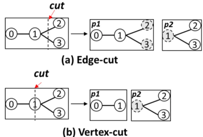
Existing main graph processing engines adopt either edge-cut [5], [6] or vertex-edge-cut [7], [17] method to partition graphs onto multiple machines by cutting them through edges or vertices, respectively. As shown in Figure 1, edge-cut replicates cross-partition edges which causes data communication between partitions. For example, when vertex 1 needs to receive data from vertex 2, there is data communication between partition p1 and p2. On the other hand, vertex-cut replicates cross-partition vertices. When vertex 1 needs data from vertex 2, the data is sent to the mirror replica of vertex 1, which is located in the same partition as vertex 2. Although it also causes communication between replicas of vertex 1, it has the benefit of maintaining data locality for vertices. Existing studies find that vertex-cut is more efficient than edge-cut for natural graphs which has a small number of vertices with very high degrees [7]. As we focus on real-world graphs which usually follow power-law degree distribution, we focus on vertex-cut in this paper.

With the increasing sizes of real-world graphs, there have been many studies proposed to provide fast and efficient partitioning for large graphs. Some studies focus on distributed graph processing in order to reduce communication cost and obtain good load balance at the same time [18], [19], [20], [21]. Among those studies, the one-pass streaming-based partitioning method has been widely adopted [22]. Xu et al. [23] propose a heterogeneity-aware streaming graph partitioning method, which considers the heterogeneous computing and communication abilities when placing graph vertices to different machines. Mayer et al. [24] propose a window-based streaming graph partitioning method which selects the best edge from a set of edges during edge assignment to improve the quality of partitioning results. However, their method cannot be applied directly to the geo-distributed graph partitioning problem, due to the both

Fig. 1: Illustrations of (a) edge-cut and (b) vertex-cut. Shaded vertices represent ghosts and mirrors respectively.

inter- and intra-DC network heterogeneities in geo-distributed DCs. Mayer et al. [10] propose an adaptive streaming graph partitioning method named GrapH, which considers the heterogeneity in vertex traffic and networking prices and aims at minimizing the communication cost during graph processing. However, GrapH is not aware of the multi-level network bandwidth heterogeneities in geo-distributed DCs, and thus can lead to large inter-DC data transfer time. Zhou et al. [25] propose a graph partitioning method, which considers the multi-level network bandwidth heterogeneities in geo-distributed DCs to optimize inter-DC data transfer time while satisfying WAN usage constraint. However, this work does not consider the price heterogeneity of geo-distributed DCs and thus can lead to high inter-DC data transfer cost even with a low WAN usage.

This paper significantly extends a preliminary conference version [25] by considering the cost efficiency of geo-distributed graph processing. Although existing works have studied the graph partitioning problem with various criteria, none of them has considered the problem with both performance and cost as optimization objectives at the same time in geo-distributed DCs, where the network bandwidth and prices are both highly heterogeneous and quite different from those within a single data center. To tackle this challenging problem, we make extensions in three major aspects. First, we reformulate the graph partitioning problem with minimizing inter-DC data transfer time as the optimization goal and monetary budget on runtime inter-DC data communication cost as the constraint. Second, to solve the new problem efficiently, we propose a cost-aware streaming partitioning heuristic to optimize the inter-DC data communication cost and propose a new partition mapping strategy to more efficiently reduce the inter-DC data transfer time while satisfying the budget constraint. Third, we extend our experiments to an additional real-world cloud platform and using a new graph with larger size.

2.3 A Motivating Example

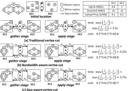
We give a simple example to demonstrate the importance of a geo-aware graph partitioning method. Figure 2 shows a graph with eight vertices, where the input data of vertices are initially

Fig. 2: A comparison between three graph partitioning methods: (a) traditional vertex-cut, (b) bandwidth-aware vertex-cut and (c) geo-aware vertex-cut. Widths of the up/down links indicate network bandwidths.

distributed in two DCs. The initial locations are selected as the master replica of each vertex. We consider three motivating partitioning methods, including a traditional vertex-cut [7], a bandwidth-aware vertex-cut [25] and the geo-aware vertex-cut method proposed in this paper.

We adopt the widely-used GAS model [7] as our graph processing model. With the vertex-centric abstraction of GAS, we can easily partition graphs using vertex-cut to parallelize vertex computations. One of the replicas for each vertex is selected as the master and all the other replicas are called mirrors. GAS model supports the bulk synchronous model of computation and there are three computation stages in each GAS iteration, namely Gather (Sum), Apply and Scatter. In the gather stage, each replica gathers data from its local neighbors and sends the gathered data to the master. The master aggre-gates all received data into the gathered sum. In the apply stage, the master updates vertex data using the gathered sum and sends the updated data to all mirrors. In the scatter stage, each replica activates its local neighbors. In this example, we assume the sum function of the graph algorithm aggregates two messages by simply binding them together and the data sizes of all vertices are the same (i.e., ai= 1 MB). The

inter-DC data transfer time can be calculated as the sum of the time spent on the gather (from mirrors to master) and apply (from master to mirrors) stages. The inter-DC data transfer cost is calculated as the sum of the data uploading cost of each DC. Assuming the budget constraint for the problem to be $0.7, we obtain the partitioning results as shown in Figure 2. We have the following observations. First, compared to the tra-ditional vertex-cut, geo-aware vertex-cut obtains both lower inter-DC data transfer time and cost. This is partly because that traditional vertex-cut is not aware of the bandwidth and

TABLE 3: Notation overview.

Symbol Meaning

M The number of geo-distributed DCs

Rv The set of DCs containing at least one replica of v

I_vr A boolean value indicating whether the replica of vertex v in

DC r is the master (Ir

v= 1) or not (Ivr= 0)

dv The input data size of vertex v

gr

v(i) The aggregated data size transfered from the mirror in DC r_{to the master of vertex v during the gather stage in iteration i}

av(i) The combined data size sent from the master of vertex v to_{each mirror in the apply stage of iteration i}

Ur/Dr Uploading/Downloading bandwidth of DC r

Pr Unit price of uploading data from DC r to the Internet

B The monetary budget of WAN usage

price heterogeneities, and tends to get a partition solution with good load balance as shown in Figure 2(a). This results in long inter-DC data transfer time at apply stage by transferring more data through the uplink of DC 1, and high inter-DC data com-munication cost at the gather stage by transferring more data via the pricy uplink of DC 2. Second, the bandwidth-aware method obtains shorter inter-DC data transfer time than geo-aware, but has higher inter-DC data communication cost due to its ignorance of the network price heterogeneity. Specifically, both methods transfer the same amount of data through WAN, while geo-aware sends less data using the pricy uplink of DC 2 and more with the cheap uplink of DC 1. This example demonstrates that it is important to consider both the network bandwidth and price heterogeneities to obtain a good trade-off between the cost and performance of geo-distributed graph processing.

0 5 10 15 20 25 0.0 0.2 0.4 0.6 0.8 1.0 Oblivious HDRF Random Grid R at i o of A c t i ve V e r t i c e s Iteration (a) PageRank 0 2 4 6 8 10 12 14 16 0.0 0.2 0.4 0.6 0.8 1.0 Oblivious HDRF Random Grid R at i o of A c t i ve V e r t i c e s Iteration (b) SSSP 0 2 4 6 0.0 0.2 0.4 0.6 0.8 1.0 Oblivious HDRF Random Grid R at i o of A c t i ve V e r t i c e s Iteration (c) SI

Fig. 3: Convergence analysis of PageRank, SSSP and SI under different strategies. The convergence speeds under the four partitioning strategies are exactly the same for SSSP and SI.

3

P

F

3.1 Model Overview

We study how to partition a large graph onto multiple geo-distributed DCs. The graph data are generated and stored geo-distributedly. For simplicity, we assume that the graph data are not replicated initially and each machine executes only one vertex replica at a time. We assume that there are unlimited computation resources in each single DC, and inter-DC data communication is the performance bottleneck of geo-distributed graph processing. This assumption is valid in the geo-distributed environment since the WAN bandwidth is much more scarce than the computation resources such as CPU and memory. We also assume that DCs are connected with a congestion-free network and the bottlenecks of the network are only from the uplinks/downlinks of DCs [13]. This assumption is based on the observation that many datacenter owners are expanding their services world widely and are very likely to build their own private WAN infrastructure [26]. We assume that only uploading data from a DC to WAN is charged. This assumption is based on the pricing scheme of most public clouds such as Amazon EC2 and Windows Azure. The graph partitioning algorithm is applied before executing graph processing algorithms.

Before formally defining the problem, we first study the impact of graph partitioning on the convergence of graph al-gorithms. We execute three graph algorithms, namely PageR-ank [27], Single Source Shortest Path (SSSP) [28] and Sub-graph Isomorphism (SI) [29], using PowerGraph engine and a synthetic power-law graph with 1,000,000 vertices (λ = 2.1). We use four existing graph partitioning strategies implemented in PowerGraph to partition the graph, namely Random [7], Grid [7], HDRF [30] and Oblivious [7]. Figure 3 shows the convergence speeds of the three graph algorithms using dif-ferent graph partitioning strategies. The convergence speed is evaluated using the ratio of active vertices among all. When a graph algorithm is converged, all vertices have finished their computation and become inactive. Interestingly, we observe that the convergence speeds are hardly affected by the parti-tioning strategies: the convergence speeds of each graph algo-rithm are almost the same when using different graph parti-tioning strategies. This means that we can optimize the perfor-mance of graph processing jobs by optimizing each processing

iteration. In the following, we model the graph processing per-formance using one iteration.

3.2 Problem Definition

Table 3 summarizes the symbols used in problem formulation. Consider a graph G(V, E) with input data stored in M geo-distributed DCs, where V is the set of vertices and E is the set of edges in the graph. Each vertex v (v = 0, 1, . . . , |V | − 1) has an initial location Lv (Lv∈ [0, 1, . . . , M − 1]), which is where

the input data of vertex v is stored.

With the distributed GAS model, the inter-DC network traf-fic mainly comes from the gather stage and the apply stage. For a given iteration i and a vertex v, each mirror in DC r sends aggregated data of size gr_v(i) to the master of v in the gather stage and the master sends the combined data of size av(i)

to each mirror to update the vertex data in the apply stage. To simplify the calculation of data transfer time, we assume there is a global barrier between the gather stage and the apply stage. Thus, the inter-DC data transfer time in iteration i can be formulated as the sum of the data transfer times in gather and apply stages. In each DC, the data transfer finishes when it is finished on both up and down links. Thus, we have:

T(i) = TG(i) + TA(i) = max r T r G(i) + max_r T r A(i) (1) TGr(i) = max( ∑ v Ivr· ∑ k∈Rv,k6=r gkv(i) Dr , ∑ v (1 − Ir v) · grv(i) Ur ) (2) TAr(i) = max( ∑ vI r v· av(i) · (|Rv| − 1) Ur , ∑ v (1 − Ir v) · av(i) Dr ) (3)

where I_vr is a boolean indicator showing whether the replica of vertex v in DC r is the master (I_vr= 1) or not (Ir

v= 0). Rv is

the set of DCs containing at least one replica of v and initial-ly contains oninitial-ly Lv. Ur and Dr are the uplink and downlink

bandwidths of DC r, respectively.

The inter-DC data communication cost is calculated as the sum of the cost on data uploading during the gather and apply stages. Denote the unit price of uploading data from DC r to the Internet as Pr, we have:

Ccomm(i) =

_∑

∑

Pr· [Ivr· dmv+ (1 − Ivr) · grv(i)] (4)

where dmv equals to av(i) · (|Rv| − 1), which represents the

Based on the above analysis, we formulate our geo-distributed graph partitioning problem as the following constrained optimization problem:

min T (i) (5)

s.t. Ccomm(i) ≤ B (6)

Note that the cost and performance objectives can be con-tradictory with each other. For example, as shown in Figure 2, the uplink of DC 2 has higher bandwidth and thus is useful for reducing the inter-DC data transfer time. However, the price of this link is also higher and hence has an adverse impact on the cost objective. Thus, it is more complicated to find a good graph partitioning solution for our problem than existing studies which consider only one of the two objectives [10], [25].

4

G

-A

G

P

In this paper, we propose a geo-aware graph partitioning al-gorithm named Geo-Cut, which incorporates two optimization stages to reduce optimization overhead. In the first stage, we study the traffic pattern during graph processing and propose a streaming heuristic which considers the network price hetero-geneity to minimize inter-DC data transfer cost. In the second stage, we propose two partition refinement heuristics which consider the network bandwidth heterogeneity to reduce the inter-DC data transfer time without violating the budget con-straint. In the following, we introduce the two optimization stages in detail.

4.1 Cost-Aware Streaming Graph Partitioning

Given the initial locations of vertices (i.e., where the input data of vertices are located), we adopt the streaming graph parti-tioning approach to quickly partition a graph. We view a graph as a stream of edges e0, . . . , e|E|−1 to be assigned to a graph

partition. The number of partitions is the same as the number of DCs. The order of edges in the set, which determines the edge that will be assigned first by the streaming partitioning method, can be decided randomly or using breadth- or depth-first traversals. Existing studies have shown that the random order of edges can produce nearly the same result as that pro-duced by optimized edge orders [31]. Thus, we randomly order the edges in the stream. One important design parameter in streaming partitioning is the heuristic which decides where to place an incoming edge. In this paper, we design a cost-aware streaming heuristic that aims at minimizing the inter-DC data communication cost.

As only the uploading network traffic is charged in geo-distributed DCs, we study the additional uploading traffic in-troduced by edge assignment. We select the initial replica of each vertex as the master replica. When placing an edge (u, v) in a DC r, it can cause two types of additional uploading traffic. First, the replication of vertex u (v) in DC r increases the uploading traffic in the initial location of u (v) by au(i)

(av(i)), which is used to synchronize the updated vertex data

between the master and the added mirror replica of u (v) in the apply stage of the GAS model. Second, the data passed along

the edge (u, v) increases the uploading data size of DC r when the mirror replicas send local aggregated data of u and/or v to the master replicas in the gather stage. Denote the aggregated data size transferred from the mirror of a vertex v in DC r to the master replica during the gather stage in iteration i as gr_v(i). We calculate the increased gathering traffic size caused by placing an edge (u, v) in DC r in iteration i as follows. Without loss of generality, we assume graphs are directed and data are gathered from in-edges.

∆gru,v(i) = Sum(grv(i), au(i − 1)) − grv(i) (7)

Based on the above analysis of graph traffic pattern, we derive the following streaming heuristic which always tries to place an incoming edge (u, v) to the DC that leads to the lowest increased inter-DC data transfer cost.

1) If Rvand Ruintersect, place edge (u, v) in any r ∈ Rv∩Ru

with the lowest C_gatherr , where

C_gatherr = (1 − I_vr) · Pr· ∆gru,v(i) (8)

2) If Rvand Rudo not intersect, place (u, v) in a DC r with

the lowest sum of C_gatherr and the synchronization cost C_syncr , where Csyncr =      PLu· au(i) if r ∈ Rv PLv· av(i) if r ∈ Ru

PLu· au(i) + PLv· av(i) otherwise

(9)

After the edge assignment, we build local subgraphs in each DC and create vertex replicas as needed. The time complexity of the streaming graph partitioning is O(|E|). As our stream-ing heuristic prioritizes DCs which do not require replicatstream-ing vertices, our partitioning method can also result in a low vertex replication rate and hence low data movement cost.

4.2 Performance-Aware Partition Refinement

After the cost-aware partitioning, in this stage, we consider the highly heterogeneous network bandwidth in geo-distributed DCs and propose two heuristics to reduce the inter-DC data transfer time while satisfying the budget constraint. First, we propose a simple yet effective partition mapping heuristic which iteratively tries to switch the mapping of partitions to reduce the inter-DC data transfer time while satisfying the budget constraint. Second, we consider the network bandwidth heterogeneity and use edge migrations to diminish the data traffic in bottlenecked DCs to further reduce the inter-DC data transfer time while satisfying budget constraint. 4.2.1 Partition Mapping

Mapping the M graph partitions to M geo-distributed DCs is a classic combinatorial NP-hard problem and has a solution space of O(M!). For small values of M, we can simply adopt BFS/DFS-based search algorithms to find the best mapping solution. Specifically, in our problem, a mapping solution is better than another when it obtains less inter-DC transfer time while satisfying monetary budget. For a large number of DCs, it is however non-trivial to design a heuristic for finding the best partition mapping due to the network heterogeneities in both bandwidths and prices.

We propose a simple yet effective algorithm for quickly finding a good graph partition mapping solution. The algo-rithm is inspired by the “power of two choices” [32] tech-nique, which has been demonstrated effective in task ing problems for finding the approximately optimal schedul-ing solution with low latency [33]. Recent studies have fur-ther discovered that using d > 2 choices can provide orders-of-magnitude improvements [34] when task sizes are heavy-tailed. Similar to task scheduling problems, our partition map-ping problem is also a balls-to-bin scheduling problem with some tailed “tasks” due to network heterogeneities. Thus, we can expect the “power of many choices” technique to be ef-fective for our problem. Our partition mapping algorithm is shown in Algorithm 1.

Algorithm 1 Graph partition mapping algorithm.

Require: Pinit: the initial partition mapping solution;

Ensure: Popt: the optimized partition mapping solution;

1: Popt= Pinit;

2: continue = true; 3: repeat

4: Randomly sample d pairs of partitions;

5: Let Gb= 0 and pb= 0;

6: for i = 1 to d do

7: (Gi, costi)=EstimateGain(pairi,Popt);

8: if Gi> Gb and costi≤ B then

9: Let Gb= Giand pb= i;

10: if Gb> 0 then

11: Switch the mapping of partitions in pairpbto generate plan Popt;

12: else 13: continue= f alse; 14: until !continue 15: return Popt; Algorithm 2 EstimateGain(pair, P) Require:

pair: the pair of partitions to be evaluated; P: the current partition mapping solution; Ensure:

G: the estimated gain of switching the pair of partitions in P;

C: the inter-DC data communication cost after switching partitions in P; 1: Let G = 0 and C = 0;

2: Generate plan P0 by switching the partition mapping of pair;

3: G = EstimateTime(P) − EstimateTime(P0);

4: C = EstimateCommCost(P0);

5: return G and C;

Starting from an initial partition mapping solution, we ran-domly select d pairs of partitions (Line 4) and estimate the gain of switching their mapping. The initial partition mapping solution can be the partitioning result obtained by the first optimization stage or an optimized solution given by any other graph partitioning method. The gain of switching the mapping of two partitions is calculated as the reduced inter-DC data transfer time if the switched partition mapping still satisfies the budget constraint (otherwise the gain is zero) (Line 7). We select the pair with the best gain among the d pairs and switch its partition mapping (Line 8-9). Iteratively, we repeat the above process until no improvement can be obtained or a predefined number of iterations has been reached. The choice of d is related to the severity of network performance hetero-geneity, which corresponds to the tail length in task scheduling problems. By default, we choose d = 2. We estimate the gain and cost of switching the mapping of two partitions using Algorithm 2. The gain is calculated as the difference between

the estimated data transfer time before and after the switching (Line 3). The data transfer time is estimated using Equation 1 which characterizes the performance of GAS model and the data transfer cost is estimated using Equation 4.

Complexity Analysis: According to Equations 1 and 4, the time complexity of Algorithm 2 is O(M). Assuming the pre-defined maximum number of iterations to sample new pairs of partitions for switching is MaxIter, the overall time complexity of our partition mapping algorithm is O(MaxIter × M), which is much faster than the naive search algorithms.

4.2.2 Edge Migration

Network bandwidth heterogeneity can cause performance bot-tlenecks even with a good partition mapping. For example, as shown in Table 1, both the uplink and downlink bandwidths of Sydney are lower than the other two cloud DCs. Thus, an equal partition of the graph workload will lead to performance bottleneck on the Sydney DC. To mitigate such performance bottlenecks, we propose to migrate edges out of the bottle-necked DCs after obtaining a good partition mapping.

According to Equations 1–3, we can identify the bottlenecks of inter-DC data communication by estimating the data trans-fer time in the gather and apply stages for each DC r, i.e., T_Gr(i) and Tr

A(i), respectively. The bottlenecks for the gather

(apply) stage are the DCs which have the same data transfer time as TG(i) (TA(i)). The bottleneck can be bounded either

on the uplink or the downlink of the DC. Thus, there can be four types of bottlenecked links, namely uplink/downlink bounded in the gather stage and uplink/downlink bounded in the apply stage. If the gather and apply stages are bounded on the same link of the same DC, we migrate edges out of that DC considering the reduction to the inter-DC data transfer time. Otherwise, we select the link with more possible reduction to the data transfer time of the gather and apply stages to migrate. Note that, in both cases, the migration is allowed only when the budget constraint is not violated.

Based on Equations 1–3, we address a bottlenecked link lr of DC r as follows. If lr is uplink and bounds the gather

stage, the network traffic on lr is mainly caused by mirror

replicas in the DC sending gathering data to the masters. Thus, we order the mirror replicas according to their gathering data sizes (i.e., gr_v(i) for the mirror of vertex v in DC r) in a priority queue Q. We iteratively remove the vertices in Q until lr is no

longer the bottleneck or Q is empty. If lris downlink and also

bounds the gather stage, the network traffic on lr is mainly

caused by master replicas receiving the gathering data from mirrors. Thus, we order the master replicas in DC r accord-ing to their non-local gatheraccord-ing data sizes. After removaccord-ing the master replicas, we select the replica with the largest number of local neighbors in each DC as the master of a vertex, in order to further reduce the inter-DC network traffic. Similarly, for bottlenecks of the apply stage, if lr is uplink (downlink),

we order the master (mirror) replicas in DC r according to the vertex data sizes. After removing a vertex replica v, we migrate each edge connected to v to a DC which results in the shortest inter-DC data transfer time. We calculate the inter-DC data transfer time after migrating an edge using Equation 5 with the updated inter-DC network traffic. By default, we migrate

one edge at a time.

Complexity Analysis: The average time complexity of the edge migration can be calculated as O(|Q| ×|E|_{|V |}× M). As |Q| is on average |V |_M, we have the time complexity as O(|E|). To balance the trade-off between the effectiveness and efficiency of edge migrations, we provide two optimizations. First, as introduced in Section 2, it is common in power-law graphs that a small portion of vertices are contributing to most of the data traffic. Thus, we can limit the length of Q to a small value LQwhile achieving similar migration results. Second, for

each vertex candidate v in Q, we group the edges connected to v into C groups, where edges in the same group will be migrated at the same time to the same DC. We adopt the clus-tering method to group edges, and the distance between two edges is defined as the intersection size between the replication locations of the other end of the edges. For example, for two edges (u, v) and (w, v), the distance between them is defined as |R(u) ∩ R(w)|. In this way, we can minimize the number of additional vertex replications and hence the size of additional inter-DC data transfer caused by edge migrations. With the two optimizations, we are able to reduce the time complexity of edge migration to O(LQ×C × M).

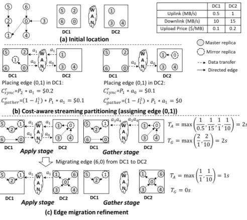
4.3 A Concrete Example

To better illustrate our two-stage optimizations method, we present a concrete example to partition a small graph with seven vertices and six edges using Geo-Cut. The initial loca-tions of the vertices are shown in Figure 4(a).

First, we apply our cost-aware streaming graph partitioning method to get an initial partitioning solution. Assume the first edge to be assigned is edge (0, 1), we show how to place it in Figure 4(b). As R0 and R1 do not intersect, according to

Equation 8 and 9, we can calculate the total increased cost of placing the edge in DC1 and DC2 to be $0.3 and $0.1, respectively. Thus, edge (0, 1) should be placed in DC2. Af-ter placing all edges using the same way, we get an initial partitioning solution for the graph.

Second, we apply the partition mapping refinement tech-nique. In this example, switching the mapping of the two par-titions does not bring any gain, so the partitioning solution remains unchanged.

Third, we identify the bottlenecks of inter-DC data commu-nication and apply the edge migration refinement. Based on equations 1–3, we calculate the time of the apply and gather stages to be both 2s, and we can identify the uplink of DC1 to be the bottleneck of the apply stage. To address this bottleneck, we order vertices 0, 2, 5 and 6 according to their data sizes. As all vertices have the same data size, we choose to remove vertex 0 and migrate edge (6, 0) from DC1 to DC2. After edge migration, the time of the apply and gather stages are reduced to 1s and 0s, respectively.

5

P

D

G

With Geo-Cut, we are able to partition a static graph in O(|E|) time, assuming |E|  M. However, many real-world graphs such as social network graphs are dynamic, with frequent vertex and edge insertions/deletions (e.g.,

newly registered/deactivated users and following/unfollowing operations). These changes to a graph can greatly affect graph partitioning decisions. For example, a deactivated celebrity Facebook user, who usually has a large number of followers, can greatly affect the network traffic of the new social network graph. Repartitioning the entire graph once changes occur is not cost-effective due to its large overhead. In the following, we discuss how to use Geo-Cut to adaptively partition dynamic graphs with a low overhead.

Since adding and removing a vertex can be represented as adding and removing edges connected to this vertex, we ab-stract the changes to a dynamic graph as edge insertions and edge deletions, assuming that a graph has no isolated vertex. It has been pointed out by existing studies [35] that a dynamic graph can be viewed as an intermediate state of the streaming graph partitioning. Thus, we can adopt the streaming graph partitioning technique of Geo-Cut to directly assign inserted edges to DCs. The challenge is that, the inserted/deleted edges can change the data traffic of vertices and thus make the exist-ing partitionexist-ing less effective. For example, when insertexist-ing a large number of edges connected to an originally low-degree vertex v, it is better to move v to a DC with high bandwidths. To address this challenge, we periodically apply our par-tition refinement technique to the updated graph parpar-titions. Specifically, we use partition mapping to relocate the graph partitions which have new edges inserted. We use the edge migration technique to migrate edges from the current bottle-necked DC to DCs which have deleted edges, if the inter-DC data transfer time can be reduced. It is costly to perform the refinement every time an edge is inserted/deleted. Thus, we need to decide the timing of partition refinement. Specifical-ly, we calculate the increased/decreased data traffic size to a partition caused by edge insertions/deletions using the same way as introduced in streaming graph partitioning. We trigger the partition refinement whenever the number of changes to data traffic caused by edge insertions/deletions is larger than a threshold. By default, we set threshold to 10% of the overall data traffic size of a partition. The time complexity of inserting a set of edges E0 is O(|E0| + MaxIter × R) and that of deleting a set of edges is O(LQ× C × R), where R is the number of

partition refinement operations applied. This is much faster than repartitioning the entire graph.

6

E

We evaluate the effectiveness and efficiency of Geo-Cut us-ing real-world graph datasets on both real clouds and a cloud simulator. We use Amazon EC2 and Windows Azure for real cloud experiments. To emulate the congestion-free network model, we limit the uplink and downlink bandwidths of the instances to be smaller than the WAN bandwidth. The limit-ed bandwidths are proportional to their original bandwidths. We adopt the GAS-based PowerGraph [7] system to execute graph processing algorithms. The evaluated graph partitioning methods are implemented using C++ programming language in PowerGraph to partition graphs while loading. We adopt a multi-threaded implementation to parallelize the streaming graph partitioning and to reduce the ingress overhead.

Fig. 4: A concrete example of applying the two-stage optimizations of Geo-Cut to partition a graph. TABLE 4: Experimented real-world graphs.

Notation #Vertices #Edges αin αout

Gnutella (GN) 8,104 26,013 2.91 2.59 WikiVote (WV) 7,115 103,689 3.63 3.80 GoogleWeb (GW) 875,713 5,105,039 2.96 3.64 LiveJournal (LJ) 3,577,166 44,913,072 3.45 2.88 Twitter (TW) 41,652,230 1,468,365,182 3.29 3.55 6.1 Experimental Setup

Graphs. We select five real-world graphs for our experiments, which are representative graphs in P2P networks, social net-works and web graphs. Table 4 gives details of the graphs [36]. Graph algorithms. We adopt three graph algorithms which are widely used in different areas, including PageRank (PR) [27], Single Source Shortest Path (SSSP) [28] and Subgraph Isomorphism (SI) [29].

PR is widely used in web information retrieval to evaluate the relative importance of webpages. SSSP finds the shortest paths starting from a single source to all other vertices in the graph. SI is used to find the subgraphs matching certain graph pattern in a large graph.

Compared methods. We compare Geo-Cut with the fol-lowing state-of-the-art vertex-cut graph partitioning methods. We adopt the original implementation of these algorithms if open-sourced1and implement our own version if otherwise.

Baseline [7] uses random hashing to assign an edge to a DC containing the source or target node of the edge. If such a DC cannot be found, it assigns the edge to a random DC. Baseline is used as the baseline comparison, as what has been done in the other compared methods [7], [10], [25].

1. https://github.com/rossojr92/PG-ObliviousGreedy-Partitioning

Greedy [7] iteratively places edges to the DCs which min-imize the expected vertex replication factor.

GrapH[10] considers the heterogeneity in vertex traffic and network pricing, and assigns edges to minimize the data com-munication cost.

G-Cut [25] is our previous work on geo-distributed graph partitioning, which considers the network bandwidth hetero-geneity to optimize graph processing performance while sat-isfying WAN usage constraint.

Configuration details. We use both real cloud experiments and simulations to evaluate the effectiveness of Geo-Cut.

Real cloud experiments.We select eight regions of Amazon EC2 as the geo-distributed DCs, namely US East (USE), US West Oregon (OR), US West North California (NC), EU Ire-land (EU), Asia Pacific Singapore (SIN), Asia Pacific Tokyo (TKY), Asia Pacific Sydney (SYD) and South America (SA). With Azure, we select four regions, including East US (US), West Japan (JP), West Europe (EU) and Southeast Australi-a (AUS). In eAustrali-ach region, we construct Australi-a cluster of five c-c2.8xlarge EC2 instances or A8-v2 Azure instances. In all experiments, we compare the performance and monetary cost of graph algorithms optimized by Geo-Cut and the four com-pared methods. As GrapH is designed to optimize the data communication cost for graph algorithms, we set the monetary budget of runtime data communication to the cost of GrapH by default. All results are normalized to those of Baseline if not otherwise specified.

Simulations.We simulate 20 geo-distributed DCs using net-work performances and prices measured from Amazon EC2. We perform three sets of simulations using Livejournal graph. First, we construct three types of geo-distributed

environ-TABLE 5: Bandwidth and price settings for the bandwidth heterogeneity experiments. Bandwidth/Price DC 0-9 DC 10-14 DC 15-19 Heter. Low 1/1 1/0.5 0.5/0.5 0.74 Medium 1/1 0.5/0.5 0.25/0.5 0.89 High 1/1 0.5/0.5 0.125/0.5 0.96

TABLE 6: Bandwidth and price settings for the price hetero-geneity experiments.

Bandwidth/Price DC 0-9 DC 10-14 DC 15-19 Heter.

Low 1/1 0.5/1 0.25/1 0

Medium 1/1 0.5/0.75 0.25/0.5 0.26

High 1/1 0.5/0.25 0.25/0.125 0.71

ments with “Low”, “Medium” and “High” network hetero-geneities and study the impact of network heterohetero-geneities on the effectiveness of Geo-Cut. Specifically, we consider two types of heterogeneities in network bandwidths and prices. We present the network and price settings of the 20 DCs for the bandwidth and price heterogeneity experiments in Tables 5 and 6, respectively. Specifically, we identify the DCs as DC 0-19. We set the network bandwith and prices of DC 0-9 to be the same as those measured from the US East Region of Amazon EC2 and change the settings of the rest proportionally to obtain different system heterogeneities. For example, for the “High” bandwidth heterogeneity environment, we change the upload/download bandwiths of DC 10-14 and 15-19 to one eighth and half of the measured bandwidths, respectively. We change the network prices of DC 10-19 to half of the original prices, to match the fact that lower bandwidths are usually cheaper in the cloud. To quantitatively define the het-erogeneity of network bandwidth, we use the relative standard deviation of the bandwidths of all links (including uplinks and downlinks) in the network as the metric. Similarly, for the heterogeneity of network prices, we use the standard deviation of the prices of all uplinks in the network as the metric. The calculated metrics in Table 5 and 6 show that the bandwidths and prices are in accordance with the heterogeneity settings.

Second, we study the impact of budget constraint on the effectiveness of Geo-Cut. We vary the budget from 1.0, 0.9, ..., to 0.6 times of the default budget and compare Geo-Cut with G-Cut [25], which is a network bandwidth heterogeneity aware graph partitioning method, to show the effectiveness of the cost-aware design in Geo-Cut on satisfying the budget constraint. For fair comparison, we set the WAN usage budget of G-Cut to the runtime WAN usage of GrapH by default. When varying the monetary budget of Geo-Cut, we vary the WAN usage budget for G-Cut accordingly in the same way. For all settings, the bandwidths and prices are set as the same as those in the “Medium” price heterogeneity environment.

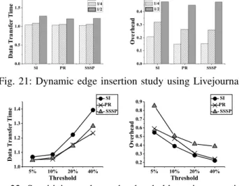
Third, we study the effectiveness of Geo-Cut on partitioning dynamic graphs under the High network bandwidth hetero-geneity. We first study the threshold parameter, which decides how often partition refinements are triggered when partition-ing dynamic graphs. With the default threshold, we consider three types of graph changes, including edge insertions, edge deletions and dynamic partitions. For edge insertions, we take 7/8, 3/4 and 1/2 of the edges in a graph as the initial static graph and insert the rest of the edges. For edge deletions, we iteratively remove 1/8, 1/4 and 1/2 of the edges from the

TABLE 7: The absolute values of inter-DC data transfer time obtained by Baseline on Amazon EC2.

Time GN WV GW LJ TW

SI 770s 2250s 7.5h 319.4h 575h

PR 3.8ms 11.7ms 136ms 5.3s 9.5s

SSSP 2ms 5.9ms 67.9ms 2.6s 4.8s

TABLE 8: The absolute values of inter-DC data transfer time obtained by Baseline on Windows Azure.

Time GN WV GW LJ TW

SI 478s 1670s 5.1h 205.8h 375h

PR 2.3ms 7.3ms 87ms 3.2s 6.2s

SSSP 1.2ms 3.6ms 43.8ms 1.6s 3.1s

initial graph. We reduce the number of partitions from 20 to 15 and reassign the edges in the removed five DCs to the rest DCs. We evaluate the effectiveness and efficiency of dynamic partition refinement.

6.2 Real Cloud Results

6.2.1 Inter-DC Data Transfer Time

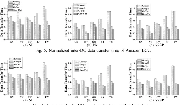
Figures 5 and 6 show the normalized inter-DC data transfer times of the compared algorithms on Amazon EC2 and Win-dows Azure, respectively. The absolute data transfer times of the baseline algorithm are shown in Table 7 and 8.

We have the following observations. First, on both clouds, Geo-Cut obtains the shortest data transfer time compared to the other methods. Specifically, on Amazon EC2, Geo-Cut re-duces the inter-DC data transfer time by 46%-79%, 25%-64%, 19%-64% and 4%-24% compared to Baseline, Greedy, GrapH and G-cut, respectively. On Windows Azure, the time reduc-tion are 46%-76%, 17%-64%, 7%-64% and 2%-13% com-pared to Baseline, Greedy, GrapH and G-Cut, respectively. Second, comparing the optimization results of different graphs, Geo-Cut obtains higher time reduction over other compared methods on graphs with more heterogeneous data communica-tions. For example, as shown in Table 4, Gnutella and WikiV-ote graphs have similar size (i.e., number of vertices) while the latter has more skewed vertex degree distribution (i.e., larger α value). As a result, the time reduction obtained by Geo-Cut for WikiVote is up to 79% (47% as the median value) on Amazon EC2 and 76% (45% as the median value) on Windows Azure, while the reduction for Gnutella is only up to 68% (34% as the median value) on Amazon EC2 and 66% (25% as the median value) on Windows Azure.

These observations demonstrate that the heterogeneity-aware graph partitioning of Geo-Cut is effective in reducing the inter-DC data transfer time for geo-distributed graph processing.

To better understand the effectiveness of each individual technique proposed in Geo-Cut, and to verify the analysis above, we further breakdown the optimization results of WikiVote graph on both Amazon EC2 and Windows Azure as shown in Figure 9, where Streaming represents optimization with the cost-aware graph partitioning technique only and Placement represents optimization with both Streaming and partition mapping technique. All results are normalized to those of Streaming. We have the following observations.

First, comparing the results obtained by Placement and Streaming, the partition mapping technique is more effective

Geo-Cut TW GW LJ (a) SI Geo-Cut TW GW LJ (b) PR Geo-Cut TW GW LJ (c) SSSP

Fig. 5: Normalized inter-DC data transfer time of Amazon EC2.

Geo-Cut TW GW LJ (a) SI Geo-Cut TW GW LJ (b) PR Geo-Cut TW GW LJ (c) SSSP

Fig. 6: Normalized inter-DC data transfer time of Windows Azure. on reducing the inter-DC data transfer time on Amazon

EC2 than that on Window Azure. Specifically, on Amazon EC2, Placement reduces the inter-DC data transfer time by 27%-35% compared to Streaming, while on Azure, the improvement obtained by partition mapping is not obvious. This is mainly because the network bandwidth heterogeneity of Amazon EC2 DCs is much higher than that of Windows Azure DCs. Specifically, the highest download/upload bandwidth is 5x/2x as high as the lowest download/upload bandwidth on Amazon EC2 and is only 1.79x/1.42x on Windows Azure. Higher bandwidth heterogeneity offers better opportunity for partition mapping to further reduce the inter-DC data transfer time. Second, comparing the results obtained by Geo-Cut and Placement, the edge migration technique is also more effective on reducing the inter-DC data transfer time on Amazon EC2 than that on Windows Azure. Specifically, on Amazon EC2, Geo-Cut reduces the inter-DC data transfer time by 13%-16% compared to Placement, while on Windows Azure, the time reduction is only 2%-6%. This is mainly due to the fact that the difference between network bandwidth and price heterogeneities on Amazon EC2 is much larger than that on Windows Azure. On Amazon EC2, the highest network price is 8x as high as the lowest network price and is only 1.38x on Windows Azure. As Streaming is only aware of the price heterogeneity when assigning edges to DCs, it is more likely to cause performance bottlenecks on Amazon EC2 DCs than on Windows Azure, where the edge migration technique can be made use of. These observations demonstrate that the techniques designed in Geo-Cut work well for geo-distributed environments with significant network bandwidth and price heterogeneities.

6.2.2 Inter-DC Data Transfer Cost

Figures 7 and 8 show the monetary costs spent on inter-DC data communication optimized by the compared algorithms. All results are normalized to the budget.

TABLE 9: Vertex replication rates optimized by compared algorithms for PageRank on Windows Azure.

Baseline Greedy GrapH G-Cut Geo-Cut

Gnutella 2.60 1.91 1.94 1.81 1.85

WikiVote 2.68 2.02 2.06 1.97 2.00

GoogleWeb 1.44 1.26 1.26 1.12 1.15

LiveJournal 3.28 2.25 2.26 1.72 1.78

Twitter 2.36 1.49 1.62 1.29 1.34

Overall, Geo-Cut obtains the lowest inter-DC data transfer cost on both clouds and is able to satisfy the budget con-straint under all settings. Specifically, Geo-Cut reduces the data communication cost by 36%-70%, 14%-53%, 1%-50% and 2%-18% compared to Baseline, Greedy, GrapH and G-Cut on Amazon EC2 and 45%-75%, 18%-55%, 6%-48% and 4%-15% compared to Baseline, Greedy, GrapH and G-Cut on Windows Azure, respectively. The reason that Geo-Cut obtains lower data communication cost lies in two aspects.

First, Geo-Cut leads to less WAN usage during graph processing compared to other partitioning methods including Baseline, Greedy and GraphH, as shown in Figures 10 and 11. SSSP obtains similar results as those of PageRank and thus is not shown in the figures. Our streaming heuristic in the streaming graph partitioning technique prefers to assign an edge to the partition which does not require vertex replication. As a result, Geo-Cut can achieve a low vertex replication rate. For example, we show the vertex replication rates optimized by the compared partitioning algorithms for PageRank on Windows Azure in Table 9. As shown in the table, vertex replication rate obtained by Geo-Cut is lower than those obtained by Baseline, Greedy and GrapH, and is comparable to that of G-Cut. This is because G-Cut is also designed for geo-distributed clouds with WAN usage as one optimization factor. Lower vertex replication rate leads to less inter-DC communications between vertex replicas and potentially lower inter-DC networking cost.

Second, in addition to reducing WAN usage, Geo-Cut can smartly distribute more data communication to DCs with lower

Geo-Cut GN WV GW LJ TW (a) SI Geo-Cut GN WV GW LJ TW (b) PR Geo-Cut GN WV GW LJ TW (c) SSSP

Fig. 7: Normalized inter-DC data transfer cost of Amazon EC2.

Geo-Cut GN WV GW LJ TW (a) SI Geo-Cut GN WV GW LJ TW (b) PR Geo-Cut GN WV GW LJ TW (c) SSSP

Fig. 8: Normalized inter-DC data transfer cost of Windows Azure.

0.0 0.2 0.4 0.6 0.8 1.0 1.2 SI PR D a t a T r a n s f e r T i m e Streaming Placement Geo-Cut SSSP

(a) Amazon EC2

0.0 0.2 0.4 0.6 0.8 1.0 1.2 SI PR D a t a T r a n s f e r T i m e Streaming Placement Geo-Cut SSSP (b) Windows Azure

Fig. 9: Normalized data transfer time optimized by traffic-aware graph partitioning only (Streaming), both Streaming and partition mapping (Placement) and Geo-Cut using WikiVote.

Geo-Cut

(a) SI

Geo-Cut

(b) PR

Fig. 10: Normalized WAN usage obtained on Amazon EC2.

Geo-Cut

(a) SI

Geo-Cut

(b) PR

Fig. 11: Normalized WAN usage obtained on Windows Azure.

TABLE 10: Uploading data distribution on Amazon EC2.

USE USW-O USW-NC EU SIN TKY SYD SA price($) 0.02 0.02 0.02 0.02 0.09 0.09 0.14 0.16 Greedy(%) 12 13 12 13 12 13 13 12 GrapH(%) 12 15 12 14 11 13 12 11 G-Cut(%) 11 11 13 13 15 12 13 12 Geo-Cut(%) 11 15 16 15 13 9 10 11

inter-DC network prices. For example, Table 10 shows the up-loading data distribution in different DCs of Amazon EC2 op-timized by the compared partitioning methods using WikiVote graph and SI algorithm. Overall, Geo-Cut distributes 57% of the total uploading data to the cheapest four DCs while Greedy is more load-balanced with 50% of the total data distributed to the cheapest four DCs. G-Cut distributes 48% of the total uploading data to the cheapest four DCs due to its ignorance of the network price heterogeneity. GrapH is also aware of the price heterogeneity and distributes 53% of the total data to the cheapest four DCs. However, due to its larger WAN usage during graph processing, GrapH still results in higher data communication cost compared to Geo-Cut.

6.2.3 Trade-off Between Performance and Cost

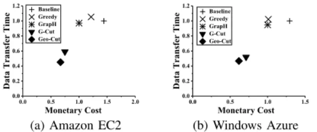
It is interesting to also study the trade-off between the perfor-mance and cost of graph processing in geo-distributed DCs. We present the inter-DC data transfer time and cost results obtained by the compared partitioning methods using Twit-ter graph and Subgraph Isomorphism algorithm in a skyline evaluation manner as shown in Figure 12. All time results are normalized to that of Baseline and the cost results are normalized to the budget. We have the following observations.

First, there is no obvious relationship between the perfor-mance and cost optimization goals. For example, on Amazon EC2, the partitioning results of GrapH and Greedy lead to almost the same inter-DC data transfer time while the data transfer cost obtained by GrapH is much lower. On the other hand, the results on Windows Azure show that GrapH and Greedy obtain almost the same inter-DC data transfer cost while the data transfer time of GrapH is slightly lower than

0.0 0.5 1.0 1.5 2.0 0.0 0.2 0.4 0.6 0.8 1.0 1.2 Baseline Greedy GrapH G-Cut Geo-Cut D at a T r an s f e r T i m e Monetary Cost

(a) Amazon EC2

0.0 0.5 1.0 1.5 0.0 0.2 0.4 0.6 0.8 1.0 1.2 Baseline Greedy GrapH G-Cut Geo-Cut D at a T r an s f e r T i m e Monetary Cost (b) Windows Azure

Fig. 12: Trade-off between inter-DC data transfer time and cost using Twitter graph and SI algorithm.

that of Greedy. This shows that the complicated bandwidth and price heterogeneities in geo-distributed DCs make it hard to optimize the performance and cost goals at the same time. Second, on both clouds, Geo-Cut is able to obtain better result when comparing both inter-DC data transfer time and monetary cost to the other methods. This is consistent with our observations in the previous two subsections where Geo-Cut is able to obtain both lower inter-DC data transfer time and lower cost than the other methods at the same time. This shows that Geo-Cut is able to obtain performance- and cost-efficient graph partitioning result in geo-distributed DCs.

6.2.4 Graph Partitioning Overhead

We evaluate the partitioning overhead of Geo-Cut using PageRank algorithm. As shown in Figure 13, we breakdown the overhead into three parts, namely the overhead spent on streaming partitioning, the overhead on partition mapping and the overhead on edge migration. We have several observations. First, the overhead of Geo-Cut is much higher than that of Greedy while is comparable to that of GrapH. For example, the partitioning overhead for the Livejournal graph is 105s with Greedy, 1720s with GrapH and 1020s with Geo-Cut. This is mainly because the heterogeneity-aware partitioning tech-niques of Geo-Cut are more complicated than Greedy.

Second, streaming partitioning takes the largest portion of the entire overhead of Geo-Cut, and the ratio increases as the graph size increases. For example, for GoogleWeb, the stream-ing partitionstream-ing overhead is only 57% of the entire overhead while for Livejournal, the ratio is over 90%. Overall, to par-tition one million edges, it takes Geo-Cut less than three sec-onds for small size graphs such as GoogleWeb and around 100 seconds for large size graphs such as Twitter.

Third, partition mapping and edge migration techniques have comparable overhead. For edge migration, the LQ

parameter, which decides the number of edges to be migrated, has significant impact on the trade-off between migration effectiveness and efficiency. We perform a sensitivity study over this parameter by varying LQ from 0%, 5%, 10%, 15%

to 20% of the number of vertices in Q. Figure 14 shows the resulted edge migration overhead and normalized inter-DC data transfer time on Amazon EC2 using Livejournal graph. As LQincreases, the effectiveness of edge migration increases

(i.e., the inter-DC data transfer time decreases) while the efficiency decreases (i.e., the migration overhead increases almost linearly). When LQ is larger than 10%, the inter-DC

data transfer time becomes stable. By default, we set LQ

to 5% to get a good balance between the effectiveness and efficiency of edge migration.

LJ 0.0 2.0x10 2 4.0x10 2 6.0x10 2 8.0x10 2 1.0x10 3 GN WV GW 0 4 8 12 16 O ve r h e ad ( s ) Streaming P artition mapping Edge migration TW 0.0 4.0x10 4 8.0x10 4 1.2x10 5 1.6x10 5

Fig. 13: Graph partitioning overhead breakdown of Geo-Cut.

0% 5% 10% 15% 20% 0 50 100 150 200 E d ge M i gr at i on O ve r h e ad ( s ) SI PR SSSP LQ 0% 5% 10% 15% 20% 0.8 0.9 1.0 1.1 D at a T r an s f e r T i m e SI PR SSSP LQ

Fig. 14: Sensitivity study of LQ on Amazon EC2 using LJ.

6.3 Simulation Results

We present the simulation results using real cloud traces to evaluate the sensitivity of Geo-Cut to different parameters, in-cluding network heterogeneities in bandwidth and prices, bud-get constraint and dynamic graph changes.

Geo-Cut

(a) SI

Geo-Cut

(b) PR

Fig. 15: Normalized inter-DC data transfer time under different bandwidth heterogeneities using Livejournal.

Geo-Cut

(a) SI

Geo-Cut

(b) PR

Fig. 16: Normalized inter-DC data transfer cost under different bandwidth heterogeneities using Livejournal.

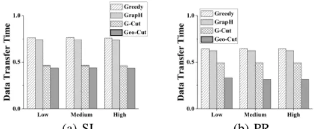
6.3.1 Network Heterogeneity

Bandwidth heterogeneity. Figure 15 and Figure 16 show the normalized inter-DC data transfer time and cost optimized by the compared algorithms under different network bandwidth heterogeneities, respectively. The time results are normalized to those of Baseline and the cost results are normalized to those of GrapH. SSSP obtains similar results as those of PageRank and thus is not shown in the figures.

Geo-Cut obtains the lowest inter-DC data transfer time among the compared methods under all settings. Specifically, Geo-Cut reduces the data transfer time over the compared methods by 4%-55%, 5%-68% and 4%-72% for the Low, Medium and High bandwidth heterogeneity environments,

Geo-Cut

(a) SI

Geo-Cut

(b) PR

Fig. 17: Normalized inter-DC data transfer time under different price heterogeneities using Livejournal.

Geo-Cut

(a) SI

Geo-Cut

(b) PR

Fig. 18: Normalized inter-DC data transfer cost under different price heterogeneities using Livejournal.

respectively. Benefiting from its bandwidth heterogeneity awareness, Geo-Cut obtains higher time reduction over Baseline, Greedy and GrapH in environments with more heterogeneous network bandwidths. This trend does not apply when comparing Geo-Cut with G-Cut, as G-Cut is also designed to be bandwidth heterogeneity aware.

Similarly, Geo-Cut obtains the lowest inter-DC data transfer cost among all compared methods (except G-Cut) under all settings. The monetary cost obtained by Geo-Cut increases slightly with the increase of network bandwidth heterogene-ity. This is because, with the increase of network bandwidth heterogeneity, the partition mapping and edge migration tech-niques have better opportunity of further reducing the inter-DC data transfer time over the results of Streaming, while sacrific-ing the monetary cost optimized by Streamsacrific-ing. For example, when the heterogeneity changes from Low to High, the two techniques obtain 44%-54% more time reduction over Stream-ing while the additional monetary cost compared to the cost optimized by Streaming increases by 8%-13%. This shows that Geo-Cut can effectively address the network bandwidth heterogeneity problem to improve the performance of geo-distributed graph processing.

To verify these observations, we also implement the band-width heterogeneity experiments with PageRank and Twitter, which is the largest graph in our paper. Specifically, Geo-Cut reduces the the data transfer time over the compared method-s by 3%-73%, 2%-77% and 3%-81% for the Low, Medium and High bandwidth heterogeneity environments, respectively. The normalized monetary cost of Geo-Cut slightly increases from 80% to 85% when the bandwidth heterogeneity changes from Low to High. These results are consistent with those obtained using Livejournal. Because of the high experimental overhead of Twitter, we use Livejournal only for the rest of the simulations.

Price heterogeneity. Figure 17 and Figure 18 show the nor-malized inter-DC data transfer time and cost optimized by the compared algorithms under different network price het-erogeneities, respectively. The time results are normalized to

1.0*B0.9*B0.8*B0.7*B0.6*B 0.9 1.2 1.5 1.8 D at a T r an s f e r T i m e Budget Geo-Cut G-Cut (a) SI 1.0*B 0.9*B 0.8*B 0.7*B 0.6*B 0.9 1.2 1.5 1.8 2.1 D at a T r an s f e r T i m e Budget Geo-Cut G-Cut (b) PR

Fig. 19: Normalized inter-DC data transfer time under different budget constraints. 1.0*B0.9*B0.8*B0.7*B0.6*B 0.5 0.6 0.7 0.8 0.9 1.0 M on e t ar y C os t / WA N U s age Budget Geo-Cut G-Cut (a) SI 1.0*B 0.9*B 0.8*B 0.7*B 0.6*B 0.5 0.6 0.7 0.8 0.9 1.0 M on e t ar y C os t / WA N U s age Budget Geo-Cut G-Cut (b) PR

Fig. 20: Monetary cost/WAN usage under different budget constraints.

those of Baseline and the cost results are normalized to those of GrapH. SSSP obtains similar results as those of PageRank and thus is not shown in the figures.

Similar to the bandwidth heterogeneity study, Geo-Cut ob-tains the lowest inter-DC data transfer time among the com-pared methods under all settings. Differently, the time reduc-tion obtained by Geo-Cut compared to the other methods does not change much with the increase of price heterogeneity. For example, Geo-Cut reduces the inter-DC data transfer time by 5%-67%, 5%-68% and 5%-68% for Low, Medium and High network price heterogeneities, respectively. This is mainly be-cause the three-stage design of Geo-Cut can guarantee good inter-DC data transfer time for different price heterogeneities. The price heterogeneity only affects the optimization result of the streaming partitioning stage, which tends to assign edges more balanced to different DCs when the price heterogeneity is low and assign more edges to less pricy DCs when the price heterogeneity is high. In the former case, the edge mi-gration method can be used to adapt to the network bandwidth heterogeneity while in the latter case, the partition mapping technique can be used to reduce the inter-DC data transfer time. The monetary cost obtained by Geo-Cut increases slight-ly with the increase of network bandwidth heterogeneity. This is because, with the increase of network price heterogeneity, the partition mapping and edge migration techniques have to sacrifice more monetary cost optimized by Streaming, in order to further reducing the inter-DC data transfer time over the results of Streaming.

6.3.2 Budget Constraint

Figure 19 shows the inter-DC data transfer time obtained by Geo-Cut and G-Cut under different budget constraints, where Brepresents the default budget. All results are normalized to those of Geo-Cut under B. Figure 20 shows the monetary cost obtained by Geo-Cut and the WAN usage obtained by G-Cut under different budget constraints. All results are normalized to their own budget. We have the following observations.