HAL Id: halshs-01599362
https://halshs.archives-ouvertes.fr/halshs-01599362
Submitted on 2 Oct 2017
HAL is a multi-disciplinary open access archive for the deposit and dissemination of sci-entific research documents, whether they are pub-lished or not. The documents may come from teaching and research institutions in France or abroad, or from public or private research centers.
L’archive ouverte pluridisciplinaire HAL, est destinée au dépôt et à la diffusion de documents scientifiques de niveau recherche, publiés ou non, émanant des établissements d’enseignement et de recherche français ou étrangers, des laboratoires publics ou privés.
Climatic variation as a determinant of rural-to-rural
migration destination choice: Evidence from Tanzania
Zaneta Kubik
To cite this version:
Zaneta Kubik. Climatic variation as a determinant of rural-to-rural migration destination choice: Evidence from Tanzania. 2017. �halshs-01599362�
Documents de Travail du
Centre d’Economie de la Sorbonne
Climatic variation as a determinant of rural-to-rural migration destination choice: Evidence from Tanzania
Zaneta KUBIK
Climatic variation as a determinant of rural-to-rural migration
destination choice: Evidence from Tanzania
Zaneta Kubik
*Abstract
This paper attempts to establish if climate acts as the determinant of destination choice in case of
rural-to-rural migration. In the context of climate change where the link between climate and rural-to-rural income has
been well established, it is argued that migrants who move within rural areas choose destinations with
more favourable climate conditions allowing for higher incomes. Employing the alternative-specific
conditional logit model, this paper shows that such indirect effect of climate on migration destination
choice is non-negligible, since one per cent increase in the expected income differentials between origin
and destination, attributable to climate, increases the probability of choosing a given destination by at
least nine percentage points. On the other hand, distance acts as a constraint for migration, in particular
for the poorest individuals who might be inhibited from reaping full benefits of mobility.
Keywords: climate change, regional migration, rural economics, agriculture, regional economics JEL classification : R11, R23, Q15, Q54
Introduction
The widespread view holds that agriculture’s vulnerability to climate change may provoke sizeable migration flows within the developing world. A growing literature has established the link between climate shocks and mobility (Millock, 2015), and even though future predictions vary greatly (Laczko and Aghazarm, 2009), there is little doubt that populations confronted with adverse climatic conditions are already taking up migration as an adaptation measure (Findley, 1994; Henry, Schoumaker & Beauchemin, 2004; Feng, Krueger & Oppenheimer, 2010; Dillon, Mueller & Salau, 2011). Rural households in developing countries are expected to be particularly vulnerable to the ongoing climate change. Not only the unprecedented variability in weather patterns will occur much earlier in the tropical low-income countries than in the rest of the world (Mora et al., 2013), but also, it will affect a larger share of populations whose livelihoods depend predominantly on smallholder rain-fed agriculture and for whom weather constitutes by far the biggest risk (Cranfield at al., 2003; Morton, 2007). With the agricultural yields predicted to fall by about 10 per cent by 2050 (Schlenker & Lobell, 2010), the low-income countries of sub-Saharan Africa are expected to experience the sharpest losses (Deryng et al., 2011; Dell, Jones & Olken, 2012).
In the context where weather fluctuations translate directly into income fluctuations, migration may be considered as a spatial diversification of income sources (Rosenzweig & Stark, 1989) allowing for higher incomes, in line with traditional migration model (Todaro, 1969; Harris & Todaro, 1970) or lower income risk, as in the New Economics of Migration framework (Stark & Levhari, 1982; Lucas & Stark, 1985; Stark & Bloom, 1985; Katz & Stark, 1986). Since agricultural activities are affected by weather deviations to a higher extent than manufacturing
(IPCC, 2007), which implies that urban incomes are somewhat better protected against weather vagaries than rural incomes, the literature has typically focused on rural-to-urban migration and the concomitant inter-sectoral mobility out of agriculture (Barrios, Bertinelli & Strobl, 2006; Marchiori, Maystadt & Schumacher, 2012; Henderson, Storeygard & Deichmann, 2014; Maurel & Tucchio, 2016). However, the evidence form several African countries has shown that rural-to-rural migration is not only a predominant form of mobility in many parts of sub-Saharan Africa (Beauchemin, 2011; Potts, 2012), but in particular, it plays a crucial role in the context of climatic shocks (Findley, 1994; Henry, Schoumaker & Beauchemin, 2004). In Tanzania, according to the data from the National Panel Survey (TZNPS) on which the present study is based, 70 per cent of rural migrants move to another rural area; and the same figure is observed in Kagera Health and Development Survey (KHDS) (Hirvonen & Lilleor, 2015). Since rural-to-urban migration entails higher cost than migration to rural areas (Henry et al., 2004) and is exposed to more legal or implicit barriers, such as information asymmetry or income risk resulting from employment probability uncertainty (de Brauw, Mueller & Lee, 2014), rural-to-rural migration may simply be more feasible in times of economic distress (Findley, 1994; Henry et al., 2004) while still displaying welfare-improving effect, as shown both in Tanzania (Beegle, de Weerdt & Dercon, 2011) as well as other African countries (de Brauw, Mueller & Woldehanna, 2013; Garlick, Leibbrandt & Levinsohn, 2016).
Taking into account the prevalence of rural-to-rural migration as a form of mobility in Tanzania as well as other countries, its welfare-improving effect deserves more attention. Indeed, from a theoretical perspective, income maximization is the principal rationale for migration (Todaro, 1969; Harris & Todaro, 1970) with the income differentials between origin and destination
considered to be a driving force of migration irrespective of whether the destination is urban or rural (de Brauw et al., 2014). On the other hand, the nature of these income differentials might differ in case of rural-to-urban and rural-to-rural migration. More specifically, with respect to the former, the traditional migration model (Todaro, 1969; Harris & Todaro, 1970) points to higher returns to labour and individual characteristics, particularly education, in urban areas relative to rural areas with the underlying assumption that geographical mobility is followed by intersectoral mobility out of agriculture and towards manufacturing or services (Lucas, 2004), and recent studies have emphasized the persistent productivity gap between agriculture and non-agricultural sectors as a catalyst of urbanization in the developing world (McMillan & Rodrik, 2011; Gollin, Lagakos & Waugh, 2011). In case of rural-to-rural migration where the scope of intersectoral mobility is negligible and migrants mostly remain engaged in agriculture after moving to a new destination, the intra-rural income differentials cannot be explained by a productivity gap between sectors. Instead, Gardner (1981) and Oberai and Bilsborrow (1984) emphasize the importance of destination’s characteristics which provide opportunities and constraints that make locations more or less attractive to individuals. Henry et al. (2004) note that environmental factors should be considered as a specific type of contextual characteristics that may influence migration decisions. In particular, since, as noted above, weather is a detrimental factor in agricultural production and plays a crucial role in rural livelihoods, it is expected that climatic variation explain income differentials between rural destinations and therefore, for rural-to-rural migrants, climate may act as a pull factor in migration choice.
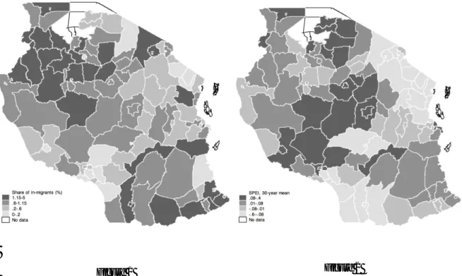
Figures (1) and (2) suggest that in Tanzania, it might be the case. Figure (1) presents the share of in-migrants per district observed in the TZNPS, pointing to a high concentration of in-migrants in North-Western and South-Eastern parts of the country. According to Figure (2), the same districts are also characterized by more favourable climatic conditions, proxied here by the 30-year mean Standardized Precipitation-Evapotranspiration Index (SPEI), where the values around zero, i.e. medium-grey colour in Figure 2, are considered to represent the most optimal conditions for plant growth and agricultural production. Therefore, it seems that indeed, climate acts as a pull factor and destinations where the observed climatic conditions are more optimal for agriculture attract higher share of migrants.
Accordingly, this paper attempts to empirically analyse if climatic variation between alternative destinations is a determinant of migration destination choice in case of rural-to-rural migration.
In the context where the link between climate and agricultural income has been well established, it is argued that for rural-to-rural migrants, of whom majority remain employed in agriculture after migration, income differentials, the rationale for migration in line with migration theory, are attributable to differences in climatic conditions between origin and destination. It is therefore expected that climate will act as a pull factor attracting rural-to-rural migrants to destinations offering more favourable climatic conditions. The analysis focuses on a sample of rural-to-rural migrants and employs the alternative-specific conditional logit model (McFadden, 1974). The results suggest that indeed, rural-to-rural migrants tend to move towards districts where climate conditions allow for higher incomes, i.e. a one per cent increase in the expected income differential, attributable to climate at a given destination, increases the probability of choice of this destination over alternative locations by nine percentage points.
The contribution of the paper is twofold. First, it adds new evidence to the scant literature on the determinants of the choice of migration destination. With the exception of Stark and Taylor (1991), Lokshin, Bontch-Osmolovski and Glinskaya (2007), Funkhouser (2009), and Fafchamps and Shilpi (2013), the question of how migrants in developing countries choose their destinations has been little studied. Second, it contributes to the literature on environmentally-induced migration by extending the analysis of climate as migration driver to show that not only does climate act as a push factor, as has typically been the focus of existing studies, also in case of Tanzania (Kubik & Maurel, 2016) but additionally, it can be a pulling force that attracts migrants to potentially more optimal destinations. To our knowledge, only Lewin, Fisher and Weber (2012) addressed, to some extent, a similar question and showed that migrants choose to move to communities where rainfall variability and drought probability are lower. The difference in this
paper is that it explicitly shows that climate acts as a pulling force indirectly through income channel. The results, apart from presenting a more complex picture of migration decision, are important in that they indicate that especially in the context of the ongoing and predicted climate change, migration may be considered as a rational, viable adaptation strategy leading to potentially better outcomes for the affected populations.
The remainder of the paper is organised as follows: the next section introduces the conceptual framework and estimation strategy. Then, the data with the descriptive statistics of main variables are presented in detail. The remaining sections demonstrate the findings. First, the income equation analysis shows that, in line with the literature, climate has a non-negligible impact on rural incomes which gives support to the assumptions on which the conceptual framework of this paper is based. Then, the main results with respect to the determinants of the rural-to-rural migration destination choice suggest that, according to the expectations, climate acts as a pull factor as more favourable climate conditions attract more migrants. The robustness checks confirm these findings. Finally, the last section concludes.
Conceptual framework and estimation strategy
The principal objective of this study is to establish whether climate acts as a determinant of migrants’ likelihood of moving to one of N possible rural destinations. Essentially, the assumption is that, with the exception of extreme events which are not analysed here, climate, rather than having a direct impact on migration choices, for example through individual preferences, affects migration destination choice through its impact on the expected income at
the destination. Indeed, migrants observed in the TZNPS never report climate as a reason to move. Instead, it is expected that destinations characterized by more favourable climate conditions guarantee higher rural incomes and therefore migrants should consider such destinations as more optimal choice. Following Fafchamps and Shilpi (2013), the model predicts that for an individual i, the probability of migrating from the original location o to destination d increases in the difference between utilities ��� − ��� , with d = {1,…, N}, and decreases in the cost of migration ���.
Assume that individual i’s utility at the origin ��� is a function of income ���, and a vector of location-specific amenities �� (Bayoh, Irwin & Haab, 2006). The income ��� is observed in the data. Similarly, the expected utility ��� is a function of the income ��� that the migrant is likely to achieve in destination d, and the amenities ��:
��� = ��(� ��, ��)
Income ���is not observable, and therefore the corresponding estimates are computed for each possible destination d, as in the equation (1):
��� = + �� + � � �+ �
where income depends on a vector of individual i’s characteristics �� but also on destinations climatic conditions � � �. Contrary to Fafchamps and Shilpi (2013), parameters α, , and do not vary by location but instead, they are estimated for all rural areas together, with the underlying assumption that the returns to individual characteristics and to climatic conditions are the same across rural areas. While this is of course a simplifying assumption, the evidence based on the TZNPS suggests that it is plausible, at least in case of agricultural income. Indeed, the Wald test indicates that the hypothesis of equality of coefficients estimated for each region
separately cannot be rejected at any conventional level of significance.1 However, the same does not apply to off-farm rural income. Besides, this assumption makes it possible to isolate the effect of climate on expected income, since for each individual i, the differences between expected incomes in alternative locations will be attributable uniquely to the differences in climate conditions observed at those destinations.
Let ���� denote individual i’s choice of destinations: ���� = if individual i migrates from location o to location d, and zero otherwise. Since the study attempts to identify the determinants of the migration destination choice, but does not seek to estimate the probability of migrating itself, by construction, the sample contains only migrants. Individuals choose the destination that provides the highest expected utility in comparison to the utility achieved at the origin, therefore the higher the difference ��� − ���, the higher the probability of migration to a given destination. On the other hand, the relative benefit of moving to another location decreases in the cost of migration ��� represented here by the physical distance between origin and destination. It might be interesting to include also a measure of social distance which, as in Fafchamps and Shilpi (2013), would take into account existing social networks, language and ethnicity; however, the data on networks in each destination are not available, while differences in language and ethnicity are not particularly relevant in case of Tanzania, where the predominant majority speaks Kiswahili and where the diversity of ethnic groups is so high that none of them can be considered as dominant in any region (Barkan, 1994).
Therefore, the probability of migration can be denoted as follows:
1
Results not reported here. Estimations of farm income equation were conducted separately for each region. Such estimations were not possible at the district level due to insufficient number of observations per alternative location in the dataset.
Pr(���� = ) = �[�(�
�� − ���|��, � � �), ���]
where � ∙ is the alternative-specific conditional logit which corresponds to McFadden’s choice model (McFadden, 1974). In this model, each individual has a single choice out of N alternative destinations. For each migrant, only the actual choice of destination is observed in the dataset; the counterfactual observations for the remaining alternative destinations are therefore generated. Since in the alternative-specific conditional logit model, each alternative per individual constitutes a single observation, the total number of observations is n (individuals) x N (alternatives). Because by construction, migrants can choose only one destination, it is necessary to cluster standard errors in order to correct for the interdependence across observations that arises as a result. Around 30 per cent of migrants move within the same district, therefore, such possibility is not excluded in the basic specification, contrary to Fafchamps and Shilpi (2013); however, the analysis including only migrants moving to district other than the district of origin is also conducted as a robustness check.
Data
Table A1 in the Annex presents the definitions and descriptive statistics for all variables used in the study. The principal source of data used in this analysis is the Tanzania National Panel survey (TZNPS) which is a nationally representative living standard survey (World Bank’s LSMS-ISA) collected by the National Bureau of Statistics (NBS). Up to date, three waves of the panel are available: 2008/09, 2010/11, and 2012/13. 16,709 individuals were interviewed at the baseline,2 and the eligible individuals were followed in the consecutive rounds with the overall
2
Since individuals who migrated between the consecutive survey rounds were re-interviewed together with all members of their new households, the total number of individuals interviewed at least once between 2008 and 2013 increased to 27,889.
attrition rate of 11 per cent between 2008 and 2013,3 which, as shown by Kubik and Maurel (2016), does not consistently bias migration analysis based on this dataset. Because the focus of the paper is on economically-driven rural-to-rural migration, the sample is limited to individuals in working age4 who resided in a rural area of mainland Tanzania5 and who permanently moved to another rural area.
The permanent character of migration is, of course, conventional and is defined here by two factors: its duration exceeding one year, and the resulting loss of the original household member status. Despite the fact that in Tanzania, where low net migration rates conceal much higher turnover (Muzzini & Lindeboom, 2008), the analysis of temporary migration would be of much interest as well, the lack of destination data on temporary migrants makes such analysis unfeasible. Migrants are identified based on the GPS coordinates6 of their respective households in each wave. In total, 696 migrants from rural areas are identified between 2008 and 2013, of whom 477 are rural-to-rural migrants and they constitute the principal focus of the analysis; however, a comparative analysis is conducted with respect to rural-to-urban migrants as well. In this setting, each migrant can choose between 112 districts of mainland Tanzania as alternative destinations7, which produces a dataset of 53,424 observations in total.
3
Individuals ages 15 years and above were eligible for re-interview. The attrition rate was 10 per cent between 2008/09 and 2010/11, and seven per cent between 2010/11 and 1012/13.
4
Between 15- and 64-year-old.
5
The choice of not including Zanzibar is dictated by two factors. First of all, the climate data used in this study is not available for islands. Second, the political, economic, and livelihood system in Zanzibar is very distinct from mainland Tanzania.
6
For confidentiality purposes, the random offset within a specified range was applied to the households GPS coordinates; however, medium- or low-resolution spatial queries should be only minimally affected by this procedure. Only individuals who moved more than 10 km are counted as migrants. Note that, by construction, it is impossible to identify migrants from the third wave.
7
A limited number of districts from coastal regions of the Indian Ocean and Lake Victoria had to be dropped from the analysis because of the lack of climate data.
The data on districts’ characteristics come from various sources. The districts’ attributes such as population density and the share of economically active individuals in the population are derived from the NBS shapefiles released with the 2002 census. The geographical distance between migrants’ original villages and the alternative districts8
is computed based on the GPS coordinates. Index of amenities is a measure of the availability of different facilities, such as primary and secondary schools, clinics, hospitals, banks, post offices, police stations or community-owned tap water; and is computed with a polychoric principal component analysis by Kolenikov and Angeles (2009) based on the data from the TZNPS’ first wave.
The climate data corresponding to each district is derived from the Standardized Precipitation Evapotranspiration Index (SPEI) dataset by Vicente-Serrano, Begueria and Lopez-Moreno (2010). SPEI is an index of monthly deviations from the average water balance, i.e. precipitations minus potential evapotranspiration, is normalized at zero, with positive values indicating wet and negative values dry conditions;9 it is therefore comparable over time and space. The advantage of SPEI over widely used measures such as temperature and rainfall lies in the fact that ‘it includes the role of temperature in drought severity by means of its influence on the atmospheric evaporation demand’ (Vicente-Serrano et al., 2010), it should therefore capture climatic conditions better than temperature and rainfall employed separately, as has typically been done in the literature. Another advantage of SPEI is that it provides the climate data in high resolution, i.e. 0.5° x 0.5°,10 which is important in a single country analysis.
8 This is a geodetic distance, i.e. the length of the shortest curve between two points (here: migrants’ original village
and alternative districts’ centroids) along the surface of a mathematical model of the Earth.
9
A SPEI equal to zero indicates a value corresponding to 50 per cent of cumulative probability of water deficit and water surplus according to log-logistic distribution (Vicente-Serrano et al., 2010).
10
The index is available at several time-scales, ranging from 1 to 48 months; in this study, the one-month SPEI is used and this choice is motivated by the fact that in the panel data setting applied for the income analysis, the use of longer time-scales, those above 12 months, causes an overlapping of climate data between years, leading to imprecise results (not reported here). In order to account for both unimodal and bimodal rainfall patterns observed in Tanzania, the monthly SPEI is averaged over the whole year. The alternative solution would be to take the January – June average to account for the most important growing season, as done by Rowhani, Ramankutty and Linderman (2011), but this gives similar results (not reported here). Alternatively, the monthly temperature and precipitation from the Climate Research Unit (CRU) dataset of University of East Anglia 11 are employed as robustness checks.
Finally, the expected income differentials between origin and alternative destinations are obtained following the strategy illustrated in the previous section, i.e. by first estimating the income regression as in equation (1) and then the coefficients from this regression being used to compute the predicted values based on individual characteristics from the TZNPS and district-level climate data described above. The income aggregates are computed employing the FAO Rural Income Generating Activities (RIGA) methodology (Quinones et al., 2009), albeit at the individual, and not the household level. Therefore, the income measure is constructed for each individual based on her participation in income-generating activities (own farm, wage-employment or self-wage-employment). All income measures are expressed in real terms, taking into account both regional and yearly differences in prices.
11
Descriptive statistics
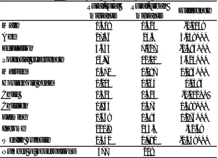
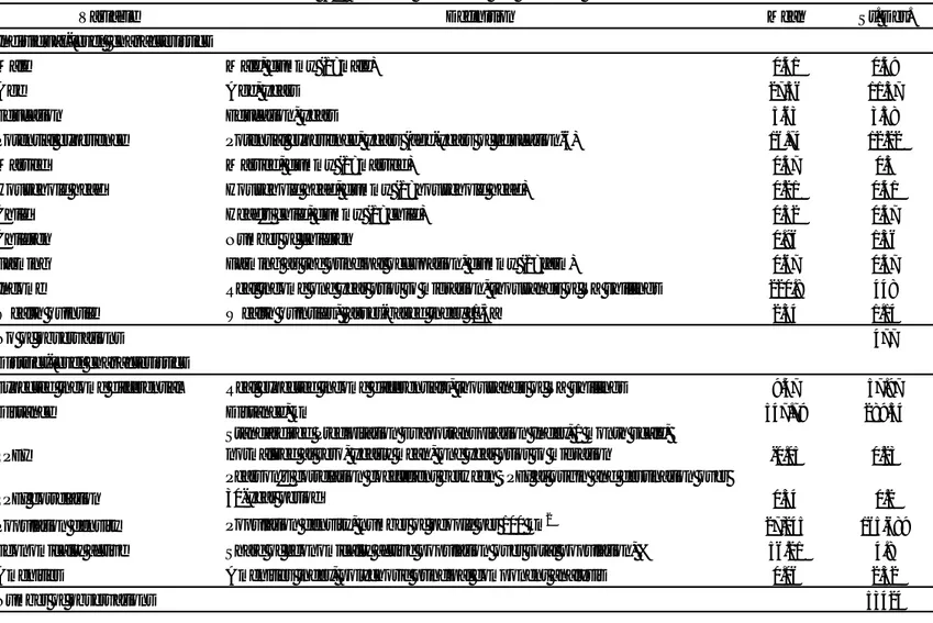
The summary statistics as well as definitions of the variables used in the study are presented in Table A1 in the Annex. Six per cent of the total sample engaged in migration between 2008 and 2013 and this seemingly low number is in line with Beegle et al. (2011) who show that mobility in Kagera region in Tanzania is lower than the potential benefits would imply. Only internal migration is observed in the TZNPS, which is consistent with the figures in the previously mentioned KHDS. As noted by Hansen (2012), there is no tradition of international migration and only three per cent of Tanzanians hold a passport. Around 70 per cent of migrants from rural areas moved to another rural area and they constitute the main sample in this study. These rural-to-rural migrants substantially differ from rural-to-urban migrants in several ways, as shown in Table 1. They are older and more likely to be married and have children, and have less years of education in comparison to rural-to-urban migrants who tend to be younger, single and better educated. More importantly, higher share of rural-to-rural migrants come from poorer households and were involved in farming as their primary activity before migration. These differences suggest that rural-to-rural and rural-to-urban migrations are very distinct processes and thus their motivations and the rationale behind the choice of destination require a separate analysis.
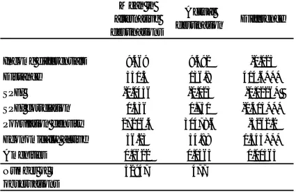
Table 2 presents a comparison between the actual destinations and the means of the remaining alternative destinations in case of rural-to-rural migration. With the mean SPEI in actual destinations higher than the mean of alternative destinations, the figures suggest that migrants tend to choose districts characterized by more favourable climate conditions that guarantee higher rural incomes, even though the difference in the expected income differentials is not statistically significant. Interestingly, climate in the actual destination is typically highly correlated with climate at the origin, contrary to the expectations from the risk minimization model as in Rosenzweig and Stark (1989); however, the distance certainly plays a role here as migrants chose relatively nearby locations. On the other hand, variables such as population density or amenities seem to be of no importance, which is not surprising in case of rural-to-rural mobility. Rural-rural migrants Rural-urban migrants Difference Male 0.409 0.425 -0.0159 Age 27.56 24.4 3.158*** Education 5.633 7.027 -1.394*** Potential experience 16.74 12.11 4.624*** Married 0.471 0.287 0.183*** Household head 0.214 0.164 0.0495 Child 0.323 0.425 -0.102** Children 0.964 0.575 0.389*** Farming 0.669 0.393 0.276*** Income 220.8 253.5 -32.69 Wealth quintile 2.342 2.781 -0.439*** Number of observations 477 219 ***p<0.01, **p<0.05,*p<0.1
Weather and income equation
Before proceeding to the estimation of migration destination choice, figures in Table 3 present the income analysis which employs a standard Mincerian equation (Mincer, 1958; Lemieux, 2006), controlling for sex, age, education, potential experience and its square term, but augmented with weather factor as in equation (1). The inclusion of weather variable is essential in order to show that climate does affect rural income, and therefore it might play a substantial role as an indirect determinant of migration destination choice for rural-to-rural migrants. The following income analysis is based on a full sample of both migrants and non-migrants observed in the three waves of the TZNPS which produces an unbalanced panel; and, as explained before, the expected income differentials used in the migration equation are computed based on these income estimates. Mean in alternative destinations Actual destination Difference Income differentials 9.469 9.492 -0.023 Distance 551.5 136.8 414.6*** SPEI -0.0456 -0.023 -0.0226* SPEI correlation 0.336 0.751 -0.415*** Population density 27216.4 30478.6 -3262.2 Economically active 56.23 54.88 1.345*** Amenities 0.0622 0.0565 0.00565 Number of observations 52947 477
Table 2. Actual and alternative destinations in rural-rural migration
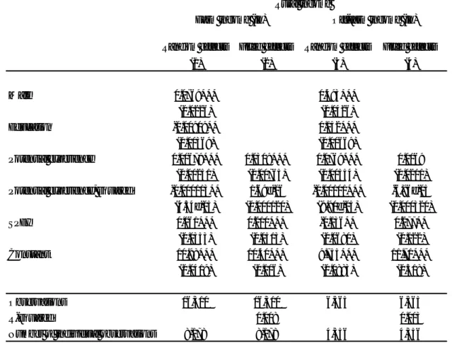
The results in column (1) for the random effects model and in column (2) for the fixed effects model confirm the importance of weather as the determinant of rural income. The fixed effects model seems to be particularly relevant to assess the impact of yearly changes in weather, and indeed, the coefficient in column (2) is highly significant, with an increase in SPEI by one standard deviation leading to an increase in rural income by about 27 per cent,12 and similar magnitude was found by Kubik and Maurel (2016). Interestingly, as shown in Table A2 in the Annex, the impact of weather on the aggregate rural income does not result uniquely from farm activities. It turns out that off-farm income, which constitutes on average around 40 per cent of
12
Note that a one standard deviation change of SPEI would entail an important change in weather conditions. For comparison, the values observed in the Tanzanian sample range from -1.06 to 0.51.
Random
effects Fixed effects
Random
effects Fixed effects
(1) (2) (3) (4) Male 0.304*** 0.686*** (0.023) (0.049) Education 0.0564*** 0.0999*** (0.004) (0.007) Potential experience 0.0695*** 0.0818*** 0.187*** 0.237*** (0.003) (0.008) (0.00540) (0.020)
Potential experience, squared -0.001*** -0.0004*** -0.00282*** -0.00161***
(0.0003) (0.0001) (0.0001) (0.0003) SPEI 0.0996*** 0.276*** -0.575*** -0.00913 (0.037) (0.057) (0.060) (0.107) Constant 10.39*** 10.21*** 8.986*** 8.828*** (0.043) (0.117) (0.096) (0.260) Observations 17,615 17,615 8,332 8,332 R-squared 0.070 0.055
Number of individual observations 8,659 8,659 4,691 4,691
Standard errors in parentheses *** p<0.01, ** p<0.05, * p<0.1
Rural income (ln) Urban income (ln)
total rural income, is affected by climate to the same extent, and this is in line with literature on the linkages between farm and off-farm activities (Baker, 1995; Karfakis, Lipper, & Smulders, 2012). For sake of comparison, the analysis of urban income is presented in columns (3) and (4); and the results from the fixed effects model suggest that weather does not have any contemporaneous effect on income in urban areas. Finally, the figures in Table 3 with respect to education, potential experience and its squared term, give support to the findings in the literature (see Lemieux, 2016 for a review); importantly, returns to education and experience are much higher in urban areas.
Main results
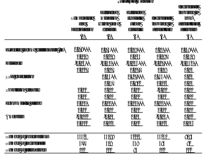
Table 4 presents the main results for the determinants of migration destination analysis and suggests that rural-to-rural migrants tend to choose destinations with more optimal climatic conditions. All the results are presented in terms of the average marginal effects, and standard errors are clustered at the individual level. Only alternative-specific characteristics, i.e. alternative destinations’ characteristics, are included in the estimations, while individual characteristics are omitted. Not only the interpretation of the effect of individual characteristics on the choice of each of the 112 alternative destinations would be of little interest for this paper, but also, a problem of endogeneity would arise in the main specification, as the expected income differentials were computed based on the same individual characteristics, such as sex, age, education or potential experience.
As explained in the conceptual framework of this paper, the assumption made in this study is that, at least in the context of developing countries, climate does not affect migration directly, for
example through individual preferences for given climatic conditions, but instead, it might be a determinant of the choice of migration destination through its influence on the expected rural income that an individual might achieve in a given destination. It is expected that destinations with more favourable climatic conditions guarantee higher incomes and therefore should be preferred over alternative destinations with less favourable climatic characteristics.
Therefore, the main specification in columns (1) and (2) controls for the expected income differentials between origin and destination as in equation (2), and, as noted in the conceptual framework, the differences between alternative destinations with respect to the expected income differentials result only from the differences in climatic conditions. The figures in column (1) suggest that the effect of expected income differentials on migration destination choice is non-negligible, since a one per cent increase in the income differentials attributable to climate increases the likelihood of choosing a given destination by nine percentage points. Note that based on the results from income equation analysis in Table 3, a slight increase in SPEI, i.e. by 0.04 standard deviation is sufficient to increase the expected income by one per cent. Not surprisingly, the effect of distance on destination choice is negative and statistically strongly significant, albeit its magnitude is rather small. Also, the share of economically active individuals in the total population is positive and statistically significant, but the magnitude of this effect is negligible. On the other hand, amenities and population density turn out not significant for rural-to-rural migrants, and this result might be in line with the literature on population density and land pressure (Jayne & Muyanga, 2012). For comparison, the same estimation is presented for rural-to-urban migrants in column (6). In line with expectations, climate does not seem to play a role as determinant of urban destinations, as the expected income
differentials are not significant anymore. Note that here, the expected income differentials capture the differences between alternative destinations, accounting for climate, but they do not represent the income differentials between rural and urban areas in general. On the other hand, and contrary to rural destinations, better access to amenities is a significant determinant of the choice of urban destinations.
Additionally, the estimations in column (2) control for the level of SPEI correlation between origin and destination over last 30 years. According to Rosenzweig and Stark (1989), households
1st 2nd 3rd
(1) (2) (3) (4) (5) (6) Expected income differentials (ln) 0.091*** 0.195*** 0.103* 0.190*** 0.140*** 0.068
0.022 0.0199 0.0594 0.0244 0.0156 0.0723 Distance -0.039*** -0.0319*** -0.060*** -0.023*** 0.003 -0.041*** 0.0012 0.008 0.004 0.0078 0.004 0.006 SPEI correlation 0.377*** 0.233* 0.241** 0.192 0.092 0.121 0.106 0.117 Population density 0.000 0.000 0.000 0.000 0.000 0.000 0.000 0.000 0.000 0.000 0.000 0.000 Economically active 0.000*** 0.000*** 0.000*** 0.000 0.000 0.000*** 0.000 0.000 0.000 0.000 0.000 0.000 Amenities -0.0012 -0.004 -0.002 -0.002 -0.0018 0.014*** 0.0010 0.0022 0.0023 0.0028 0.0028 0.003 Number of observations 53424 53424 53424 53424 53424 24528 Number of individuals 477 477 477 477 477 219 Number of alternatives 112 112 112 112 112 112
Standard errors in parentheses *** p<0.01, ** p<0.05, * p<0.1 Distance reported in hundreds of km.
Results reported in terms of average marginal effects.
Rural-urban migration By wealth tertiles
Table 4. Determinants of migration destination choice
send migrants towards destinations in which weather is not highly correlated with the origin in order to minimize income risk. On the other hand, it is plausible that locations with highly correlated weather belong to the same agro-climatic zones, and therefore rural-to-rural migrants specialized in agriculture might find it easier to migrate towards destinations with similar agro-climatic conditions in line with their agricultural specialization (Bazzi, Gaduh, Rothenberg, & Wong, 2014). The figures in column (2) give support to the latter argument and show that migrants choose destinations where climate is highly correlated with the origin. It might also be that climate similarity between locations is correlated with the distance between them; however, the results remain unchanged even after dropping the distance variable from the estimation.13 Interestingly, controlling for climate correlation between origin and destination leads to a two-fold increase magnitude of the expected income differentials; giving even more credence to the argument that moving to a destination with similar agro-climatic characteristics is more optimal from the income-maximization perspective.
Finally, in order to account for financial constraints in migration, equation (2) is estimated separately for each tertile of wealth distribution. The wealth distribution is computed based on household asset-based wealth index observed prior to migration. The results reported columns (3) – (5) show that income differentials are significant for each group, albeit with substantial differences in magnitudes of the effect. In particular, the effect of expected income differentials is almost twice higher for the individuals in the middle of wealth distribution than for the poorest ones. It is plausible that this difference results from the dependence between climate and distance, as typically, the greater the geographical proximity, the greater similarity in climate conditions and therefore, the lower income differentials between origin and destination. Indeed,
13
the findings suggest that the distance, a proxy of migration cost, is a constraint for the two lower tertiles, and particularly so for the poorest individuals, but not for the richest individuals. These results point to the interplay between potential income gains and migration cost which inhibits the poorest individuals from reaping full benefits of mobility.
Robustness checks
Finally, in order to confirm the robustness of the findings, several tests are presented in Table 5. In column (1), the expected income differentials are computed using monthly temperature and precipitation form the CRU dataset instead of SPEI, and the coefficient remain highly significant. Column (2) makes reference to Fafchamps and Shilpi (2013) who excluded the possibility of migration within the same district. The estimations based on a sample of migrants who moved to a district other than their district of origin show that such specification does not substantially alter the results with respect to the effect of the expected income differentials. On the other hand, the magnitude of the coefficient of SPEI correlation is much lower, which is plausible since climate is typically highly correlated within geographical proximity, and by not taking into account migration within the same district, the destination where climate is most correlated with the origin are dropped from the analysis. In a similar vein, column (3) excludes from alternative destinations set the districts that are mostly urban, which, by definition, are less likely to be chosen as rural-to-rural migration destination. Indeed, the magnitude of the expected income differentials’ coefficient is slightly higher, but overall, the results do not change. Lastly, in columns (4) and (5), the analysis is conducted separately for the individuals who remain involved in agriculture after migration and those who leave agriculture. Not surprisingly, the expected income differentials, attributable to climate, have much stronger impact on individuals
involved in farming, but the coefficient remains significant, albeit two times lower, for individuals who diversify out of agriculture. This is in line with the findings in Table A2 presented before suggesting that in rural areas, even the off-farm is affected by weather. On the other hand, SPEI correlation is significant only for farmers, giving more credence to the idea that individuals specialized in agriculture choose to move within similar agro-climatic conditions (Bazzi et al., 2014). Temperature and precipitation Excluding migration within same district Excluding typically urban districts Individuals involved in agriculture Individuals involved in non-agricultural activities (1) (2) (3) (4) (5)
Expected income differentials (ln) 0.178*** 0.173*** 0.209*** 0.20*** 0.138***
0.0019 0.0219 0.0154 0.0197 0.0409 Distance -0.006** -0.031*** -0.0236*** -0.027*** -0.0342** 0.0027 0.007 0.0077 0.009 0.015 SPEI correlation 0.133** 0.427*** 0.444*** 0.125 0.057 0.0912 0.1016 0.114 Population density 0.000 0.000 0.000 -0.000 0.000 0.000 0.000 0.000 0.000 0.000 Economically active 0.000* 0.000** 0.000*** 0.000*** 0.000 0.000 0.000 0.000 0.000 0.000 Amenities -0.0002 -0.004 0.003 -0.005* 0.002 0.0002 0.0025 0.002 0.0026 0.0036 Number of observations 53424 34188 42206 44240 9184 Number of individuals 477 308 449 395 82 Number of alternatives 112 111 94 112 112
Standard errors in parentheses *** p<0.01, ** p<0.05, * p<0.1 Distance reported in hundreds of km.
Results reported in terms of average marginal effects.
Table 5. Robustness checks
Conclusion
This paper attempts to establish if climate acts as a determinant of destination choice in case of rural-rural migration. In the context of the ongoing and predicted climate change where the link between climate and agricultural income has been well established, it is argued that migrants move to rural areas choose destinations with more favourable climate conditions which guarantee higher incomes. Employing the alternative-specific conditional logit model, this paper shows that such indirect effect of climate on migration destination choice is indeed non-negligible, as a one per cent increase in the expected income differential between origin and destination, attributable to climate, increases the probability of choosing a given destination by at least nine percentage points.
Rural-rural migrants also tend to choose destinations with agro-climatic conditions similar to those in the original location, in line with their agricultural specialization, and the results suggest that this might be more optimal in terms of income maximization. These findings are important in that they show that especially in the context of climate change and its growing impact on rural livelihoods, migration may be considered as a rational, viable strategy. On the other hand, distance acts as a constraint for migration, in particular for the poorest individuals, who might be inhibited from reaping full benefits of mobility. Therefore, in the context of climate change, rural-to-rural migration, currently omitted from the policy debate, should be recognised as an adaptation strategy and included into official climate policies. It is necessary to facilitate mobility across rural areas by, for example, addressing land tenure challenges and increasing the adaptive capacity of agriculture.
Bibliography
Baker, J. (1995). Survival and accumulation strategies at the rural-urban interface in north-west Tanzania. Environment and Urbanization, 7, 117-132.
Barnum, H.N., & Sabot, R.H. (1977). Education, employment probabilities and rural-urban migration in Tanzania. Oxford Bulletin of Economics and Statistics, 39, 109-126.
Barrios, S., Bertinelli, L., & Strobl, E. (2006). Climatic change and rural–urban migration: The case of sub-Saharan Africa. Journal of Urban Economics, 60, 357-371.
Bayoh, I., Irwin, E.G., & Haab, T. (2006). Determinants of Residential Location Choice: How Important Are Local Public Goods in Attracting Homeowners to Central City Locations? Journal
of Regional Science, 46, 97-120.
Bazzi, S., Gaduh, A., Rothenberg, A., & Wong, W. (2014). Skill transferability, migration, and development: evidence from population resettlement in Indonesia. Unpublished paper.
Beauchemin, C. (2011). Rural-urban migration in West Africa: towards a reversal? Migration trends and economic situation in Burkina Faso and Côte d’Ivoire. Population, Space and Place, 17, 47-72.
Beegle, K., de Weerdt, J, & Dercon, S. (2011). Migration and Economic Mobility in Tanzania: Evidence from a Tracking Survey. The Review of Economics and Statistics, 93, 1010–1033. Collier, P. (1979). Migration and Unemployment: A Dynamic General Equilibrium Analysis Applied to Tanzania. Oxford Economic Papers, 31, 205-236.
Cranfield, J.A.L., Eales, J.S., Hertel, T.W., & Preckel, P.V. (2003). Model selection when estimating and predicting consumer demands using international cross section data, Empirical
Economics, 28, 353 – 364.
de Brauw, A., Mueller, V., & Woldehanna, T. (2013). Does Internal Migration Improve Overall Well-Being in Ethiopia? Ethiopia Strategy Support Program Working Paper No. 55, Washington, D.C.: International Food Policy Research Institute.
De Brauw, A., Mueller, V., & Lee, H.L. (2014). The Role of Rural–Urban Migration in the Structural Transformation of Sub-Saharan Africa. World Development, 63, 33-42.
Dell, M., Jones, B., & Olken, B. (2012). Temperature Shocks and Economic Growth: Evidence from the Last Half Century. The American Economic Journal, 4, 66-95.
Deryng, D., Sacks, W. J., Barford, C. C., & Ramankutty, N. (2011). Simulating the effects of climate and agricultural management practices on global crop yield, Global Biogeochemical
Dillon, A., Mueller, V., & Salau, S. (2011). Migratory responses to Agricultural Risk in Northern Nigeria. American Journal of Agricultural Economics, 93, 1048-1061.
Fafchamps, M., & Shilpi, F. (2013). Determinants of Choice of Migration Destination. Oxford
Bulletin of Economics and Statistics, 75, 388-409.
Feng, S., Krueger, A. B., & Oppenheimer, M. (2010). Linkages among climate change, crop yields and Mexico–US cross-border migration. Proceedings of the National Academy of
Sciences, 107, 14257-14262.
Findley, S. E. (1994). Does Drought Increase Migration? A Study of Migration from Rural Mali during the 1983 – 1985 Drought. International Migration Review, 28, 539-553.
Funkhouser, E. (2009). The Choice of Migration Destination: A Longitudinal Approach Using Pre-Migration Outcomes. Review of Development Economics,13, 626–640.
Gardner, R. (1981). Macrolevel influences on the migration decision process. In de Jong, G., & Gardner, R. (Eds.), Migration decision making: Multidisciplinary approaches to microlevel
studies in developed and developing countries. New York: Pergamon Press.
Garlick, J., Leibbrandt, M., & Levinsohn, J. (2016). Individual Migration and Household Incomes. NBER Working Paper No. 22326.
Gollin, D., Lagakos, D., & Waugh, M. (2011). The agricultural productivity gap in developing countries. Working paper. Williams College.
Hansen, P. (2012). Revisiting the Remittance Mantra: A Study of Migration–Development Policy Formation in Tanzania. International Migration, 50, 77-91.
Harris, J. R., & Todaro, M. P. (1970). Migration, Unemployment & Development: A Two-Sector Analysis. The American Economic Review, 60, 126-142.
Henderson, J. V., Storeygard, A., & Deichmann, U. (2014). 50 Years of Urbanization in Africa: Examining the Role of Climate Change. World Bank Policy Research Working Paper 6925. Henry, S., Schoumaker, B., & Beauchemin, C. (2004). The Impact of Rainfall on the First Out-Migration: A Multi-level Event-History analysis in Burkina Faso. Population and Environment, 25, 423-460.
Hirvonen, K., & Lilleør, H. (2015). Going Back Home: Internal Return Migration in Rural Tanzania. World Development, 70, 186–202.
IPCC (2007). Climate Change 2007 – Impacts, Adaptation and Vulnerability Contribution of
Working Group II to the Fourth Assessment Report of the IPCC. Cambridge: Cambridge
Jayne, T. S., & Muyanga, M. (2012). Land Constraints in Kenya’s Densely Populated Rural Areas: Implications for Food Policy and Institutional Reform. Food Security, 4, 399–421. Katz, E., & Stark, O. (1986). Labor Migration and Risk Aversion in Less Developed Countries.
Journal of Labor Economics, 4, 134-149.
Kolenikov, S., & Angeles, G. (2004). The use of discrete data in PCA: Theory, simulations, and
applications to socioeconomic indices (Working Paper No. 04-85, MEASURE/Evaluation
project). Chapel Hill: University of North Carolina.
Kubik, Z., & Maurel, M. (2016). Weather Shocks, Agricultural Production and Migration: Evidence from Tanzania. Journal of Development Studies, 52, 665-680.
Laczko, F. & Aghazarm, C. (eds.) (2009). Migration, Environment and Climate Change:
Assessing the Evidence. Geneva: International Organization for Migration.
Lemieux, T. (2003). The “Mincer Equation” Thirty Years after Schooling, Experience and
Earnings. Center for Labor Economics, University of California, Berkeley, Working Paper No.
62.
Karfakis, P., Lipper, L., & Smulders, M. (2012). The assessment of the socio-economic impacts of climate change at household level and policy implications. In Meybeck, A., Lankoski, J., Redfern, S., Azzu, N., & Gitz, V. (eds.). Building Resilience for Adaptation to Climate Change in the Agriculture Sector. Proceedings of a Joint FAO/OECD Workshop 23–24 April 2012. Lokshin, M., Bontch-Osmolovski, M., & Glinskaya, E. (2007). Work-Related Migration and Poverty Reduction in Nepal. World Bank Policy Research Working Paper 4231.
Lucas, R. E. B. & Stark, O. (1985). Motivations to Remit: Evidence from Botswana. Journal of
Political Economy, 93, 901 – 918.
Lucas, Robert E. Jr. (2004). Life Earnings and Rural-Urban Migration. Journal of Political
Economy, 112, 29-59.
Marchiori, L., Maystadt, J. F., & Schumacher, I. (2012). The impact of weather anomalies on migration in sub-Saharan Africa. Journal of Environmental Economics and Management, 73, 355-374.
Maurel, M., & Tucchio, M. (2016).Climate Instability, Urbanisation and International Migration. Journal of Development Studies, 52, 735-752.
McFadden, D. L. (1974). Conditional logit analysis of qualitative choice behavior. In
Frontiers in Econometrics, ed. P. Zarembka, 105–142. New York: Academic Press.
McMillan, M., & Rodrik, D. (2011). Globalization, structural change, and productivity growth. NBER Working Paper No. 17143.
Millock, K. (2015). Migration and Environment. Annual Review of Resource Economics, 7, 35-60.
Mincer, J. (1958). Investment in Human Capital and Personal Income Distribution, Journal of
Political Economy, 66, 281-302.
Mora, C., Frazier, A. G. , Longman, R. J., Dacks, R. S., Walton, M. M., Tong, E. J., … Giambelluca, T. W. (2013). The projected timing of climate departure from recent variability.
Nature, 502, 183-195 (10 October 2013).
Morton, J. F. (2007). The impact of climate change on smallholder and subsistence agriculture.
PNAS, 104,19680–19685.
Muyanga, M., & Jayne, T. S. (2014). Effects of rising rural population density on smallholder agriculture in Kenya. Food Policy, 48, 98–113.
Muzzini, E., & Lindeboom, W. (2008). The Urban Transition in Tanzania. Building the Empirical Base for Policy Dialogue. Washington, DC: World Bank.
Oberai, A., & Bilsborrow, R. (1984). Theoretical perspectives on migration. In Bilsborrow, R. Oberai, A., & Standing G., (Eds.). Migration surveys in low income countries: Guidelines
for survey and questionnaire design. London & Sidney: Croom Helm.
Potts, D. (2012). Challenging the Myths of Urban Dynamics in Sub-Saharan Africa: The Evidence from Nigeria. World Development, 40, 1382-1393.
Quinones, E.J., de la O-Campos, A.P., Rodrigues-Alas, C., Hertz, T., & Winters, P. (2009). Methodology for Creating the RIGA-L Database. Prepared for the Rural Income Generating Activities (RIGA) Project of the Agricultural Development Economics Division, Food and Agriculture Organization, December 2009.
Rosenzweig, M.R., & Stark, O. (1989). Consumption Smoothing, Migration, and Marriage: Evidence from Rural India. Journal of Political Economy, 97, 905-926.
Schlenker, W., & Lobell, D. (2010).Robust negative impacts of climate change on African agriculture. Environmental Research Letters, 5.
Stark, O., & Bloom, D. (1985). The new economics of labor migration. American Economic
Review, 75, 173-178.
Stark, O., & Levhari, D. (1982). On Migration and Risk in LDCs. Economic Development and
Cultural Change, 31, 191-196.
Stark, O., & Taylor, J. E. (1991). Migration Incentives, Migration Types: The Role of Relative Deprivation. The Economic Journal, 101, 1163-1178.
Todaro, M.P. (1979). Urbanization in developing nations: trends, prospects and policies. Journal
of Geography, 79, 164-174.
Vicente-Serrano, S.M., Begueria, S., & Lopez-Moreno, J.I. (2010).A Multiscalar Drought Index Sensitive to Global Warming: The Standardized Precipitation Evapotranspiration Index. Journal
of Climate, 23, 1696-1718.
World Bank (2014). Who Wants a Job? The Magnetic Power of Cities. Tanzania Economic
Variable Definition Mean St. Dev.
Male Male, dummy (1=male) 0.41 0.49
Age Age, years 27.56 11.37
Education Education, years 5.63 3.58
Potential experience Potential experience, years (age-years of education-6) 16.74 12.22
Married Married, dummy (1=married) 0.47 0.5
Household head Household head, dummy (1=household head) 0.21 0.41
Child Head's child, dummy (1=child) 0.32 0.47
Children Number of children 0.96 1.36
Farming Farming as the principal occupation, dummy (1=farm) 0.67 0.47
Income Real income one year prior to migration, thousands of TZ shillings 220.8 448
Wealth quintile Wealth quintiles, asset-based index [1,5] 2.34 1.14
No of observations 477
Expected income differential Real expected income differentials, thousands of TZ shillings 9.47 57.97
Distance Distance, km 547.79 289.54
SPEI
Standardized Precipitation Evapotranspiration Index, 1 month scale,
normalized at zero, yearly mean, one year prior to migration -0.05 0.23
SPEI correlation
Pearson's correlation coefficient between SPEI at origin and destination over
30-year period 0.34 0.2
Population density Population density, number of people per 100 km2 27,245 165,689
Economically active Share of economically active population over total population, % 56.21 4.8
Amenities Amenities index, polychoric principal component analysis 0.06 2.32
Number of observations 53424
Table A1. Variables definitions and summary statistics
Individual-level characteristics
Random effects Fixed effects Random effects Fixed effects (1) (2) (3) (4) Male 0.0769*** 0.493*** (0.0226) (0.0426) Education -0.00909** 0.152*** (0.00369) (0.00669) Potential experience 0.00679*** 0.0309*** 0.0769*** 0.0169 (0.00251) (0.00765) (0.00554) (0.0211)
Potential experience, squared -0.000113** 1.69e-06 -0.00101*** -6.96e-05
(4.54e-05) (0.000120) (9.90e-05) (0.000320) SPEI 0.161*** 0.210*** -0.136** 0.277** (0.0353) (0.0513) (0.0680) (0.122) Constant 10.98*** 10.40*** 9.755*** 11.71*** (0.0419) (0.106) (0.0883) (0.318) Observations 16,310 16,310 6,565 6,565 R-squared 0.008 0.003
Number of individual observations 8,178 8,178 4,356 4,356
Standard errors in parentheses *** p<0.01, ** p<0.05, * p<0.1
Farm income (ln) Off-farm income (ln)
Rural income Table A2. Weather and farm and off-farm income