,! i<L::!t'... ,.'%, "
'
.:.
:r"0,.:
B'yFH.',1O |~t
'"At'~"r-..i~: i j's, .,,CusT-,: '9 .s 3LOGY
CAM'E¢~R
IXt;. takCH
USFEs
C_159,
_
U.S.A.
CONCATENATED CODES
G. DAVID FORNEY, JR.
TECHNICAL REPORT 440
DECEMBER I, 1965
MASSACHUSETTS INSTITUTE OF TECHNOLOGY
RESEARCH LABORATORY OF ELECTRONICS
CAMBRIDGE, MASSACHUSETTS
__11_ __i _1_1______
-4
The Research Laboratory of Electronics is an interdepartmental laboratory in which faculty members and graduate students from numerous academic departments conduct research.
The research reported in this document was made possible in part by support extended the Massachusetts Institute of Tech-nology, Research Laboratory of Electronics, by the JOINT SERV-ICES ELECTRONICS PROGRAMS (U. S. Army, U. S. Navy, and U. S. Air Force) under Contract No. DA36-039-AMC-03200(E);
additional support was received from the National Science Founda-tion (Grant GP-2495), the NaFounda-tional Institutes of Health (Grant MH-04737-05), and the National Aeronautics and Space Adminis-tration (Grants NsG-334 and NsG-496).
Reproduction in whole or in part is permitted for any purpose of the United States Government.
MASSACHUSETTS INSTITUTE OF TECHNOLOGY RESEARCH LABORATORY OF ELECTRONICS
Technical Report 440 December 1, 1965
CONCATENATED CODES
G. David Forney, Jr.
Submitted to the Department of Electrical Engineering, M. I. T., March 31, 1965, in partial fulfillment of the requirements for the degree of Doctor of Science.
(Manuscript received April 2, 1965)
Abstract
Concatenation is a method of building long codes out of shorter ones; it attempts to meet the problem of decoding complexity by breaking the required computation into manageable segments. We present theoretical and computational results bearing on the efficiency and complexity of concatenated codes; the major theoretical results are the following:
1. Concatenation of an arbitrarily large number of codes can yield a probability of
error that decreases exponentially with the over-all block length, while the decoding complexity increases only algebraically; and
2. Concatenation of a finite number of codes yields an error exponent that is
infe-rior to that attainable with a single stage, but is nonzero at all rates below capacity. Computations support these theoretical results, and also give insight into the rela-tionship between modulation and coding.
This approach illuminates the special power and usefulness of the class of Reed-Solomon codes. We give an original presentation of their structure and properties, from which we derive the properties of all BCH codes; we determine their weight dis-tribution, and consider in detail the implementation of their decoding algorithm, which we have extended to correct both erasures and errors and have otherwise improved. We show that on a particularly suitable channel, RS codes can achieve the performance specified by the coding theorem.
Finally, we present a generalization of the use of erasures in minimum-distance decoding, and discuss the appropriate decoding techniques, which constitute an inter-esting hybrid between decoding and detection.
TABLE OF CONTENTS
I. INTRODUCTION 1
1. 1 Coding Theorem for Discrete Memoryless Channels 1
1. 2 Concatenation Approach 3
1.3 Modulation 4
1.4 Channels with Memory 5
1.5 Concatenating Convolutional Codes 6
1. 6 Outline 6
II. MINIMUM-DISTANCE DECODING 7
2. 1 Errors-Only Decoding 7
2. 2 Deletions-and-Errors Decoding 10
2. 3 Generalized Minimum-Distance Decoding 12
2. 4 Performance of Minimum Distance Decoding Schemes 16
III. BOSE-CHAUDHURI-HOCQUENGHEM CODES 25
3. 1 Finite Fields 25
3.2 Linear Codes 28
3. 3 Reed-Solomon Codes 31
3.4 BCH Codes 34
IV. DECODING BCH CODES 38
4. 1 Introduction 38
4. 2 Modified Cyclic Parity Checks 40
4. 3 Determining the Number of Errors 41
4.4 Locating the Errors 42
4.5 Solving for the Values of the Erased Symbols 45
4. 6 Implementation 47
V. EFFICIENCY AND COMPLEXITY 51
5. 1 Asymptotic Complexity and Performance 51
5. 2 Coding Theorem for Ideal Superchannels 57
5. 3 Performance of RS Codes on the Ideal Superchannel 60
5. 4 Efficiency of Two-Stage Concatenation 68
VI. COMPUTATIONAL PROGRAM 75
6. 1 Coding for Discrete Memoryless Channels 75
6. 2 Coding for a Gaussian Channel 82
6. 3 Summary 88
CONTENTS
APPENDIX A
APPENDIX B
Variations on the BCH Decoding Algorithm
Formulas for Calculation
Acknowledgment References 39 95 102 103
I. INTRODUCTION
It is almost twenty years since Shannon announced the coding theorem. The
prom-ise of that theorem was great: a probability of error exponentially small in the block length at any information rate below channel capacity. Finding a way of implementing even moderately long codes, however, proved much more difficult than was imagined at first. Only recently, in fact, have there been invented codes and decoding methods powerful enough to improve communication system performance significantly yet simple enough to be attractive to build. 2-4
The work described here is an approach to the problem of coding and decoding
com-plexity. It is based on the premise that we may not mind using codes from 10 to 100
times longer than the coding theorem proves to be sufficient, if, by so doing, we arrive
at a code that we can implement. The idea is basically that used in designing any large
system: break the system down into subsystems of a size that can be handled, which can be joined together to perform the functions of the large system. A system so designed may be suboptimal in comparison with a single system designed all of a piece, but as long as the nonoptimalities are not crippling, the segmented approach may be the preferred engineering solution.
1. 1 CODING THEOREM FOR DISCRETE MEMORYLESS CHANNELS
The coding theorem is an existence theorem. It applies to many types of channels,
but generally it is similar to the coding theorem for block codes on discrete memoryless
channels, which will now be stated in its most modern form.5
A discrete memoryless channel has I inputs xi, J outputs yj, and a characteristic
transition probability matrix ji Pr(yj/xi). On each use of the channel, one of the
inputs xi is selected by the transmitter. The conditional probability that the receiver
then observes the output yj is Pji; the memorylessness of the channel implies that these probabilities are the same for each transmission, regardless of what happened on any
other transmission. A code word of length N for such a channel then consists of a
sequence of N symbols, each of which comes from an I-symbol alphabet and denotes one of the I channel inputs; upon the transmission of such a word, a received word of length N becomes available to the receiver, where now the received symbols are from a
J-symbol alphabet and correspond to the channel outputs. A block code of length N and
rate R (nats) consists of eNR code words of length N. Clearly eNR < IN; sometimes we
shall use the dimensionless rate r, 0 r 1, defined by Ir N = e or R = r in I.
The problem of the receiver is generally to decide which of the eNR code words was sent, given the received word; a wrong choice we call an error. We shall assume that all code words are equally likely; then the optimal strategy for the receiver in principle, though rarely feasible, is to compute the probability of getting the received word, given each code word, and to choose that code word for which this probability is
great-est; this strategy is called maximum-likelihood decoding. The coding theorem then
1
asserts that there exists a block code of length N and rate R such that with maximum-likelihood decoding the probability of decoding error is bounded by
Pr(e) e- NE(R),
where E(R), the error exponent, is characteristic of the channel, and is positive for all rates less than C, called capacity.
(PURGATED BOUND UNEXPURGATED BOUND BOUND CURVED BOUND 0.2 0.4 0.6 RATE ( IN BITS ) 0.8 0.92
Fig. 1. E(R) curve for BSC with p = . 01.
Figure 1 shows the error exponent for the binary symmetric channel whose cross-over probability is . 01 - that is, the discrete memoryless channel with transition
prob-ability matrix = Pll 2 2 = .99 P12 = 2 1 = .01- As is typical, this curve has three
segments: two convex curves joined by a straight-line segment of slope -1. Gallager5
has shown that the high-rate curved segment and the straight-line part of the error exponent are given by
11
z Q-Zm v
E(R) = max {E o(P,p)-p R}
O<p<l
P
where
J -I 1+p
Eo(P, p) -In PiP I/(
j=l i=1
P being any I-dimensional vector of probabilities Pi; this is called the unexpurgated error exponent, in deference to the fact that a certain purge of poor code words is involved in the argument which yields the low-rate curved segment, or expurgated error
exponent. An analogous formula exists for the exponent when the inputs and outputs form
continuous rather than discrete sets. It should be mentioned that a lower bound to Pr(e) is known which shows that in the range of the high-rate curved segment, this exponent
is the true one, in the sense that there is no code which can attain Pr(e) e NE (R) for
E*(R) > E(R) and N arbitrarily large.
Thus for any rate less than capacity, the probability of error can be made to
decrease exponentially with the block length. The deficiencies of the coding theorem are
that it does not specify a particular code that achieves this performance, nor does it offer an attractive decoding method. The former deficiency is not grave, since the
rel-atively easily implemented classes of linear codes6 and convolutional codes7 contain
members satisfying the coding theorem. It has largely been the decoding problem that has stymied the application of codes to real systems, and it is this problem which
con-catenation attempts to meet.
1. 2 CONCATENATION APPROACH
The idea behind concatenated codes is simple. Suppose we set up a coder and
decoder for some channel; then the coder-channel-decoder chain can be considered from the outside as a superchannel with exp NR inputs (the code words), exp NR outputs (the
decoder's guesses), and a transition probability matrix characterized by a high proba-bility of getting the output corresponding to the correct input. If the original channel is memoryless, the superchannel must be also, if the code is not changed from block to block. It is now reasonable to think of designing a code for the superchannel of length n,
dimensionless rate r, and with symbols from an e NR-symbol alphabet. This done,
we can abandon the fiction of the superchannel, and observe that we have created a code for the original channel of length nN, with (eNR)Nr code words, and therefore rate rR
(nats). These ideas are illustrated in Fig. 2, where the two codes and their associated
coders and decoders are labelled inner and outer, respectively.
By concatenating codes, we can achieve very long codes, capable of being decoded
by two decoders suited to much shorter codes. We thus realize considerable savings in
complexity, but at some sacrifice in performance. In Section V we shall find that this
3
SUPERCODER I SUPERDECODER
I OUTER INNER RAW INNER OUTER
ICODER CODER CHANNEL DECODER DECODER
'
~
SUPERCHANNELFig. . Illustrating concatenation.
sacrifice comes in the magnitude of the attainable error exponent; however, we find that the attainable probability of error still decreases exponentially with block length for all
rates less than capacity.
The outer code will always be one of a class of nonbinary BCH codes called Reed-Solomon codes, first because these are the only general nonbinary codes known, and second, because they can be implemented relatively easily, both for coding and for
decoding. But furthermore, we discover in Section V that under certain convenient
suppositions about the superchannel, these codes are capable of matching the
per-formance of the coding theorem. Because of their remarkable suitability for our
application, we devote considerable time in Section III to development of their struc-ture and properties, and in Section IV to the detailed exposition of their decoding algorithm.
1. 3 MODULATION
The functions of any data terminal are commonly performed by a concatenation of devices; for example, a transmitting station might consist of an analog-to-digital
con-verter, a coder, a modulator, and an antenna. Coding theory is normally concerned
only with the coding stage, which typically accepts a stream of bits and delivers to the
modulator a coded stream of symbols. Up to this point, only the efficient design of this
stage has been considered, and in the sequel this concentration will largely continue, since this problem is most susceptible to analytical treatment.
By a raw channel, we mean whatever of the physical channel and associated terminal
equipment are beyond our design control. It may happen that the channel already exists
in such a form, say, with a certain kind of repeater, that it must be fed binary symbols,
and in this case the raw channel is discrete. Sometimes, however, we have more
free-dom to choose the types of signals, the amount of bandwidth, or the amount of diversity to be used, and we must properly consider these questions together with coding to arrive at the most effective and economical signal design.
When we are thus free to select some parameters of the channel, the channel con-templated by algebraic coding theory, which, for one thing, has a fixed number of inputs
theory, usually described under the headings modulation theory, signal design, and
detection theory, is then appropriate. Few general theoretical results are obtainable
in these disciplines, which must largely be content with analyzing the performance of various interesting systems. Section VI reports the results of a computational search for coding schemes meeting certain standards of performance, where both discrete raw
channels and channels permitting some choice of modulation are considered. This gives considerable insight into the relationship between modulation and coding. In particular it is shown that nonbinary modulation with relatively simple codes can be strikingly superior either to complicated modulation with no coding, or to binary modulation with complicated binary codes.
1.4 CHANNELS WITH MEMORY
Another reason for the infrequent use of codes in real communication systems has
been that real channels are usually not memoryless. Typically, a channel will have long
periods in which it is good, causing only scattered random errors, separated by short bad periods or bursts of noise. Statistical fluctuations having such an appearance will be observed even on a memoryless channel; the requirement of long codes imposed by the coding theorem may be interpreted as insuring that the channel be used for enough transmissions that the probability of a statistical fluctuation bad enough to cause an
error is very small indeed. The coding theorem can be extended to channels with
mem-ory, but now the block lengths must generally be very much longer, so that the channel has time to run through all its tricks in a block length.
If a return channel from the receiver to the transmitter is available, it may be used to adapt the coding scheme at the transmitter to the type of noise currently being
observed at the receiver, or to request retransmission of blocks which the receiver
cannot decode.9 Without such a feedback channel, if the loss of information during
bursts is unacceptable, some variant of a technique called interlacing is usually
envi-sioned.1 0 In interlacing, the coder codes n blocks of length N at once, and then
trans-mits the n first symbols, the n second symbols, and so forth through the n Nth
symbols. At the receiver the blocks are unscrambled and decoded individually. It is
clear that a burst of length b n can affect no more than one symbol in any block, so
that if the memory time of the channel is of the order of n or less the received block of nN symbols will generally be decodable.
Concatenation obviously shares the burst-resistant properties of interlacing when the memory time of the channel is of the order of the inner code block length or less, for a burst then will usually affect no more than one or two symbols in the outer code,
which will generally be quite correctable. Because of the difficulty of constructing
ade-quate models of real channels with memory, it is difficult to pursue analysis of the burst resistance of concatenated codes, but it may be anticipated that this feature will prove useful in real applications.
5
-1. 5 CONCATENATING CONVOLUTIONAL CODES
We shall consider only block codes henceforth. The principles of concatenation are
clearly applicable to any type of code. For example, a simple convolutional code with
threshold decoding is capable of correcting scattered random errors, but when channel errors are too tightly bunched the decoder is thrown off stride for awhile, and until it
becomes resynchronized causes a great many decoding errors. From the outside, such
a channel appears to be an ideal bursty channel, in which errors do not occur at all
except in the well-defined bursts. Very efficient codes are known for such channels,
and could be used as outer codes. The reader will no doubt be able to conceive of other
applications. 1. 6 OUTLINE
This report consists of 6 largely self-sufficient sections, with two appendices. We
anticipate that many readers will find that the material is arranged roughly in inverse order of interest. Therefore, we shall outline the substance of each section and the con-nections between them.
Section II begins with an elaborate presentation of the concepts of minimum-distance decoding, which has two purposes: to acquaint the reader with the substance and utility of these concepts, and to lay the groundword for a generalization of the use of erasures
in minimum-distance decoding. Though this generalization is an interesting hybrid
between the techniques of detection and of decoding, it is not used subsequently.
Section III is an attempt to provide a fast, direct route for the reader of little
back-ground to an understanding of BCH codes and their properties. Emphasis is placed on
the important nonbinary Reed-Solomon codes. Though the presentation is novel, the only
new results concern the weight distribution of RS codes and the implementation of much shortened RS codes.
Section IV reports an extension of the Gorenstein-Zierler error-correcting algorithm
for ECH codes so that both erasures and errors can be simultaneously corrected. Also,
the final step in the GZ algorithm is substantially simplified. A close analysis of the complexity of implementing this algorithm with a computer concludes this section, and
only the results of this analysis are used in the last two sections. Appendix A contains
variants on this decoding algorithm of more restricted interest.
Section V contains our major theoretical results on the efficiency and complexity of concatenated codes, and Section VI reports the results of a computational program
eval-uating the performance of concatenated codes under a variety of specifications. The
reader interested chiefly in the theoretical and practical properties of these codes will
turn his attention first to Sections V and VI. Appendix B develops the formulas used in
II. MINIMUM-DISTANCE DECODING
We introduce here the concepts of distance and minimum-distance codes, and discuss
how these concepts simplify decoding. We describe the use of erasures, and of a new
generalization of erasures. Using the Chernoff bound, we discover the parameters of these schemes which maximize the probability of correct decoding; using the Gilbert bound, we compute the exponent of this probability for each of three minimum-distance decoding schemes over a few simple channels.
2. 1 ERRORS-ONLY DECODING
In Section I we described how an inner code of length N and rate R could be concat-enated with an outer code of length n and dimensionless rate r to yield a code of
over-all length- nN and rate rR for some raw channel. Suppose now one of the enNrR words
of this code is selected at random and transmitted -how do we decode what is received? The optimum decoding rule remains what it always is when inputs are equally likely: the maximum-likelihood decoding rule. In this case, given a received sequence r of length nN, the rule would be to compute Pr(rlf) for each of the enNrR code words f.
The whole point of concatenation, however, is to break the decoding process into
manageable segments, at the price of suboptimality. The basic simplification made
pos-sible by the concatenated structure of the code is that the inner decoder can decode
(make a hard decision on) each received N-symbol sequence independently. In doing so,
it is in effect discarding all information about the received N-symbol block except which
of the eN R inner code words was most likely, given that block. This preliminary
proc-essing enormously simplifies the task of the outer decoder, which is to make a final
choice of one of the enNrR total code words.
Let q = e NR When the inner decoder makes a hard decision, the outer coder and
decoder see effectively a q-input, q-output superchannel. We assume that the raw
chan-nel and thus the superchanchan-nel are memoryless. By a symbol error we shall mean the
event in which any output but the one corresponding to the input actually transmitted is
received. Normally, the probability of symbol error is low; it is then convenient to
assume that all incorrect transmissions are equally probable - that is, to assume that the transition probability matrix of the superchannel is
p
P
= (1)
Pji 1
- , i= j
where p is the probability of decoding error in the inner decoder, hence of symbol error
in the superchannel. We call a channel with such a transition probability matrix an ideal
superchannel with q inputs and probability of error p.
Recall that the maximum-likelihood rule, given r, is to choose the input
sequence f for which the probability of receiving r, given f, is greatest. When
7
·___ __· _ I _·C__II_
--the channel is memoryless, n
Pr(r
If)
=1I
Pr(ri lf i).i=l
But since log x is a monotonic function of x, this is equivalent to maximizing n
log
1i
Pr(ri fi ) = log Pr(ri fi). (2)i=l
Now for an ideal superchannel, substituting Eqs. 1 in Eq. 2, we want to maximize n a' (ri, fi), (3) i=l where log (l-p), ri = fi a' (ri, fi) -log I I) ri fi
Define the Hamming weight a(r i,fi) by
(, ri = f.1
a(ri, fi r*f (4)
ri i
Since
p
a'(rifi ) = log (-p) + lo (q)(-p) a(ri, fi)
maximizing Eq. 3 is equivalent to maximizing
P n
n log (l-p) + og (q-1)(1-p) E a(ri f).
i=l
Under the assumption p/(q-1) (l-p), this is equivalent to minimizing
n i=l
dH(r,f) is called the Hamming distance between r and f, and is simply the number of
places in which they differ. For an ideal superchannel, the maximum-likelihood
decoding rule is therefore to choose that code word which is closest to the received word in Hamming distance.
Although this distance has been defined between a received word and a code word, there is no difficulty in extending the definition to apply between any two code words. We then define the minimum distance of a code as the minimum Hamming distance between
any two words in the code.
A code with large minimum distance is desirable on two counts. First, as we shall now show, it insures that all combinations of less than or equal to a certain number t
of symbol errors in n uses of the channel will be correctable. For, suppose f is sent
and t symbol errors occur, so that ri * fi in t places. Then from Eq. 5
dH(r,f) = t. (6)
Take some other code word g. We separate the places into three disjoint sets, such that
SO if fi = gi
iE Sc if fi gi and r f (7)
Se if fi gi and ri * fi'
We note that the set Se can have no more than t elements. Now the distance between r and g,
n
dH(r, g) = a(ri, gi)
i=l
=E a(ri,gi) + a(ri,gi) + a(ri,gi), (8)
iES 0 iES c iESe
e can be lower-bounded by use of the relations
a(r i g i) a a(gi fi) = 0, i E S
a(ri, gi) = a(gi, fi) = 1, i E Sc (9)
a(ri gi) > a(gi, fi) - 1 = 0, i E Se
Here, besides Eqs. 7, we have used a 0 and the fact that for i E Sc, ri # gi.
Substi-tuting (9) in (8) yields
dH) (gf) - Se > d - t. (10)
Here, we have defined ISe
I
as the number of elements in Se and used the fact thatdH(g,f) > d if g and f are different words in a code with minimum distance d. By com-bining (6) and (10) we have proved that
dH(r,f) < dH(r,g) if t < d. (11)
9
--In other words, if to is the largest integer such that 2t0 < d, it is impossible for any combination of to or fewer symbol errors to cause the received word to be closer to any
other code word than to the sent word. Therefore no decoding error will occur.
Another virtue of a large minimum distance follows from reinterpreting the
argu-ment above. Suppose we hypothesize the transmission of a particular code word; given
the received word, this hypothesis implies the occurrence of a particular sequence of errors. If this sequence is such that the Hamming distance criterion of Eq. 11 is sat-isfied, then we say that the received word is within the minimum distance of that code
word. (This may seem an unnecessarily elaborate way of expressing this concept, but,
as in this whole development, we are taking great pains now so that the generalizations of the next two sections will follow easily.) Furthermore, the preceding argument shows that there can be no more than one code word within the minimum distance of the
received word. Therefore, if by some means the decoder generates a code word that
it discovers to be within the minimum distance of the received word, it can without fur-ther ado announce that word as its maximum-likelihood choice, since it knows that it is impossible that there be any other code word as close or closer to the received word. This property is the basis for a number12-15 of clever decoding schemes proposed recently, and will be used in the generalized minimum-distance decoding of section 2. 3.
A final simplification that is frequently made is to set the outer decoder to decode
only when there is a code word within the minimum distance of the received word. Such
a scheme we call errors-only decoding. There will of course in general be received
words beyond the minimum distance from all code words, and on such words an errors-only decoder will fail. Normally, a decoding failure is not distinguished from a decoding error, although it is detectable while an error is not.
2. 2 DELETIONS-AND-ERRORS DECODING
The simplifications of the previous section were bought, we recall, at the price of denying to the outer decoder all information about what the inner decoder received except
which of the inner code words was most probable, given that reception. In this and the
following section we investigate techniques of relaying somewhat more information to the outer decoder, hopefully without greatly complicating its task. These techniques are generalizations of errors-only decoding, and will be developed in the framework that has been introduced.
We continue to require the inner decoder to make a hard decision about which code word was sent. We now permit it to send along with its guess some indication of how reliable it considers its guess to be. In the simplest such strategy, the inner decoder indicates either that its guess is fully reliable or completely unreliable; the latter event
is called a deletion or erasure. The inner decoder normally would delete whenever the
evidence of the received word did not clearly indicate which code word was sent; also, a decoding failure, which can occur in errors-only decoding, would be treated as a dele-tion, with some arbitrary word chosen as the guess.
In order to make use of this reliability information in minimum distance decoding, we define the Elias weight by
0O, ri reliable and r = f
b(rif) , ri erased (12)
1, ri reliable and ri ~ fi
16
where is an arbitrary number between zero and one. Then the Elias distance
between a received word r and a code word f is defined as n
dE(r,f) - b(ri, fi). (13)
i=l
Note that Elias distance is not defined between two code words.
We shall let our decoding rule be to choose that code word which is closest in Elias distance to the received word. Let us then suppose that some word f from a code of minimum (Hamming) distance d is transmitted, and in the n transmissions (i) s
dele-tions occur, and (ii) t of the symbols classed as reliable are actually incorrect. Then
dE(r,f) = t + ps. (14)
Take some other code word g. We separate the places into disjoint sets such that
SO if fi = gi
Sc if fi ' gi, ri = fi rireliable
i E (15)
Sd if fi t gi' ri deleted
Se if fi gi, ri * fi, ri reliable
Note that
Isel4 t
and (16)
Isdl s.
Now the distance between r and g can be lower-bounded by the relations
b(ri, gi) > a(gi, fi)= i S0
b(ri, gi) = a(gi,fi) = 1, i E Sc
(17)
b(ri gi) = a(gi,fi) - 1 + P = , i E Sd
b(ri, gi) > a(gi, fi) - 1 = i E Se
11
where we have used Eqs. 12Z and 15. Now n
dE(r ') = b(ri'gi)
i= 1
E- a(gi.fi) + a(gi,fi) + [a(gi fi)- 1 +P] + [a(gifi) -I]
iSo iES i Sd iESe
dH(f g) - (1-3) Sd - ISe
d - (1-P)s - t, (18)
where we have used Eqs. 13, 16, 17 and the fact that the minimum Hamming distance
between two code words is d. From Eqs. 14 and 18, we have proved that
dE(r,g)> dE(r,f) if t + s < d - (I-P)s - t or t + s < d. (19)
(The vanishing of P shows why we took it to be arbitrary.) Thus with a decoding rule
based on Elias distance, we are assured of decoding correctly if t + s < d, in perfect
analogy to errors-only decoding. When we decode only out to the minimum distance
-that is, when the distance criterion of (19) is apparently satisfied - we call this dele-tions -and-errors decoding.
That erasures could be used with minimum distance codes in this way has long been recognized, but few actual decoding schemes have been proposed. One of our chief con-cerns in Section III will be to develop a deletions-and-errors decoding algorithm for the
important class of BCH codes. There we find that such an algorithm is very little more
complicated than that appropriate to errors-only decoding. 2. 3 GENERALIZED MINIMUM-DISTANCE DECODING
A further step in the same direction, not previously investigated, is to permit the
inner decoder to classify its choice in one of a group of J reliability classes Cj, 1 < j J,
rather than just two as previously. We define the generalized weight by
P~cjs ri in class C. and r = fi
c' d P r. in class C. and r. f. (2
where 0 pcj < [ej s< 1. It will develop that only the difference
a. - .
J ej - cj
of these weights is important; a will be called the reliability weight or simply weight
corresponding to class C.. We have 0 a. < 1; a large weight corresponds to a class
we consider quite and a small weight to a class considered unreliable; indeed,reliable,
if a < ak we shall say class Cj is less reliable than Ck. The case aj = 0 corresponds to an erasure, and of a. = 1 to the fully reliable symbols of the preceding section.
Let us now define a generalized distance n
dG(r,f)- c(rfi)
i=1
(21)
Again we suppose the transmission of some word f from a code of minimum distance d, and the reception of a word in which ncj symbols are received correctly and placed in
class Cj, and nej are received incorrectly in Cj. Then
J
dG(r, f) = [nej ej+ncj Pcj
j=1
Take some other code word g, and
(22)
define the sets So, Scj, and Sej by
So if fi
i l Scj if fi
Sej if fi
= gi
gi' ri = fi', ri in class Cj
A gi, ri * fi' ri in class Cj
Note that
Iscj < ncj
(24) Sej I -< nej.
Using Eqs. 20 and 23, we have
c(r i g i) a(gi, f i) = 0,
c(ri,gi) = a(gi,fi) - 1 + e= Pej'
c(ri, gi) ~ a(gi, fi) - 1 + pcj = cj
0
i E S
i E Sej,
where the second relation depends on ri = fi : gi', i E Scj. Now
n
dG(r,g) = b(r i gi)
i=l
(25)
J
> > a(gi fi) + (a(gi'fi)-l+Pej)+
iESo 0~~~~~~~~~~~~~~~~~~~j=1 EScj
I
iES (a(gi, fi)- l+pcj) 13 (23)J dG(, g)= dH(fg)- [(1-3ej)IScjl+(-Pcj eJS1 j=1 J d - [(13ej )n+ -cj cj)nej] (26) j=l
Thus, using Eqs. 22 and 26, we have proved that J dG(r,g)> dG(r,f) if [(1-.ej+3cj)ncj+(1-P j+ ej)n j] < d, j=l J or E [(1-aj)ncj +(1+aj)nej ]< d. (27) j=l
Therefore if generalized distance is used as the decoding criterion, no decoding error will be made whenever ncj and nej are such that the inequality of (27) is satisfied. When in addition we decode only out to the minimum distance - that is, whenever this inequal-ity is apparently satisfied - we say we are doing generalized minimum-distance decoding.
This generalization is not interesting unless we can exhibit a reasonable decoding
scheme that makes use of this distance criterion. The theorem that appears below shows
that a decoder which can perform deletions-and-errors decoding can be adapted to per-form generalized minimum-distance decoding.
We imagine that for the purpose of allowing a deletions-and-errors decoder to work on a received word, we make a temporary assignment of the weight a! = 1 to the set of reliability classes Cj for which j E R, say, and of the weight a! = 0 to the remaining
reliability classes Cj, j E E, say. This means that provisionally all receptions in the
classes Cj, j E, are considered to be erased, and all others to be reliable. We then
let the deletions-and-errors decoder attempt to decode the resulting word, which it will be able to do if (see Eq. 27)
2 1 nej + (ncj+nej)<d. (28)
j R j E
If it succeeds, it announces some code word which is within the minimum distance
according to the Elias distance criterion of (28). We then take this announced word and
see whether it also satisfies the generalized distance criterion of (27), now with the
original weights aj. If it does, then it is the unique code word within the minimum
dis-tance of the received word, and can therefore be announced as the choice of the outer decoder.
We are not guaranteed of succeeding with this method for any particular provisional
assignment of the a!. The following theorem and its corollary show, however, that a
J
small number of such trials must succeed if the received word is within the minimum distance according to the criterion of Eq. 27.
Let the classes be ordered according to decreasing reliability, so that aj a ak if
j < k. Define the J-dimensional vector
a (al, a2,..., a a).
Let the sets Ra consist of all j a, and Ea of all j a + 1, 0 < a < J. Let-a' be the
a a a
J-dimensional vector with ones in the first a places and zeros thereafter, which
repre-sents the provisional assignment of weights corresponding to R = Ra and E = Ea. The
idea of the following theorem is that a' is inside the convex hull whose extreme points
are the a, while the expression on the left in Eq. 27 is a linear function of a, which
must take on its minimum value over the convex hull at some extreme point - that is, at
one of the provisional assignments a'.a
J
THEOREM: If Y [(l-aj)ncj+(l+aj)nej] < d and aj > ak for j < k, there is some
j=l
a J
integer a such that 2 , nej + E (ncj+nej)<d.
j=1 j=a+l
Proof: Let J
f(a) -E [(1-aj)ncj+(l+aj)nej].
j=l
Here, f is clearly a linear function of the J-dimensional vector a. Note that
a J
f(a') a 2 C "ej I Enej + (nc+ne.).cj ej
j=1 j=a+l
We prove the theorem by supposing that f(aa) > d, for all a such that 0 a < J, and
exhibiting a contradiction. For, let
o 1- a a - aa - aa+1, 1 < a < J - 1 aJ a lJ' We see that J
o
_a
- 1, 0 a < J, and X = 1 a=0 15so that the X can be treated as probabilities. But now a J a = X a. a a a0 a=O Therefore
(4
\4J
J f(a) = f X Xaf(a ) d Xa = d. =0 a=O a=OThus if f(a') > d, all a, then f(a) > d, in contradiction to the given conditions.
There-_ a
fore f(aa ) must be less than d for at least one value of a. Q. E. D.
The import of the theorem is that if there is some code word which satisfies the generalized distance criterion of Eq. 27, then there must be some provisional assignment in which the least reliable classes are erased and the rest are not which will enable a
deletions-and-errors decoder to succeed in finding that code word. But a
deletions-and-errors decoder will succeed only if there are apparently no deletions-and-errors and d - 1 erasures, or one error and d - 3 erasures, and so forth up to to errors and d - 2to - 1 erasures,
where to is the largest integer such that 2to • d - 1. If by a trial we then mean an
oper-ation in which the d - 1 - 2i least reliable symbols are erased, the resulting provisional word decoded by a deletions-and-errors decoder, and the resulting code word (if the decoder finds one) checked by Eq. 27, then we have the following corollary.
COROLLARY: t + 1 (d+1)/2 trials suffice to decode any received word that is
within the minimum distance by the generalized distance criterion of (27), regardless of how many reliability classes there are.
The maximum number of trials is then proportional only to d. Furthermore, many
of the trials - perhaps all - may succeed, so that the average number of trials may be appreciably less than the maximum.
2. 4 PERFORMANCE OF MINIMUM-DISTANCE DECODING SCHEMES
Our primary objective now is to develop exponentially tight bounds on the probability of error achievable with the three types of minimum-distance decoding discussed above, and with these bounds to compare the performance of the three schemes.
In the course of optimizing these bounds, however, we shall discover how best to
assign the weights a to the different reliability classes. Since the complexity of the
decoder is unaffected by the number of classes which we recognize, we shall let each distinguishable N-symbol sequence of outputs yj form a separate reliability class, and
let our analysis tell us how to group them. Under the assumption, as usual, that all
code words are equally likely, the task of the inner decoder is to assign to the received yj an xj and an aj, where x is the code word x for which Pr(yj Ix) is greatest, and a
a. The Chernoff Bound
We shall require a bound on the probability that a sum of independent, identically distributed random variables exceeds a certain quantity.
The bounding technique that we use is that of Chernoffl7; the derivation which follows
is due to Gallager. 18 This bound is knownl9 to be exponentially tight, in the sense that
*
no bound of the form Pr(e) -e n E , where E is greater than the Chernoff bound
expo-nent, can hold for arbitrarily large n.
Let yi, 1 i n, be n independent, identically distributed random variables, each
with moment-generating function
g(s) s y- Pr(y) esy
and semi-invariant moment-gene rating function (s) - In g(s).
Define Ymax to be the largest value that y can assume, and
y - yPr(y)
Let Y be the sum of the yi, and let Pr(Ysn6) be the probability that Y exceeds n6, where
Ymax - 6 y. Then
Pr(Y-n6) = Pr(Yly 2,... ,yn) f(ylY... ,n),2
where
1, Y =yi n
~
>nn6f(YlY2-,Yn) =
{O otherwise.
Clearly, for any s >- 0, we can bound f by
f(Yl'Y2,. . Yn) < e[Y-n]. Then - sY -ns6 -ns6 n sy i Pr(Y>,n6) =f e e e e i=l -ns n syi = e i=l = e-n[s6-l(s)] s 0 17 _I ___IC__
where we have used the fact that the average of a product of independent random
vari-ables is the product of their averages. To get the tightest bound, we maximize over s,
and let
E(6)-- max [s6-i(s)]. s>O
Setting the derivative of the bracketed quantity to zero, we obtain g'(s)
= '(s) = g(s) .
It can easily be shown that I'(0) =, . (oo) = Ymax' and that p'(s) is a monotonically
increasing function of s. Therefore if Ymax > 6 >y-, there is a non-negative s for
which 6 = '(s), and substitution of this s in (s6-~i(s)) gives E(6).
As an example, which will be useful later, consider the variable y which takes on
the value one with probability p and zero with probability 1 - p. Then
s g(s)=p e + 1-p S pe 6 = '(s) = s pe +1 -p s 6 p e T - P 1-6 p 6(l-p) 1 - p E(6) = 6 In p(6) - In 1-= - 6 In p - (1-6) In (-p) - JC (6), where JC(6) - 6 In 6 - (1-6) In (1-6). Then if 1 6 >p, Pr(Y>n6) e-n[-61np-(1-6)ln (1-p)-JC(6)]
This can be interpreted as a bound on the probability of getting more than n6 occur-rences of a certain event in n independent trials, where the probability of that event in a single trial is p.
From this result we can derive one more fact which we shall need. Let p = 1/2, then n Pr(Y>n6)= (n 2-n 2 -nenj(6) i=n6 It follows that (nn) < enJ(6) 18
b. Optimization of Weights
We now show that the probability of decoding error or failure for minimum-distance decoding is the probability that a certain sum of independent identically distributed ran-dom variables exceeds a certain quantity, and therefore that we can use the Chernoff bound.
Let a code word from a code of length n and minimum distance d be transmitted. We know already that a minimum-distance decoder will fail to decode or decode
incor-rectly if and only if
E [ncj (1-a)+nej (1 +a] d (29)
for, in the case of errors-only decoding, all a = 1; of deletions-and-errors decoding,
aj = 0 or 1; and of generalized minimum-distance decoding, 0 a 1.
Under the assumption that the channel is memoryless and that there is no correla-tion between inputs, the probabilities Pcj of a correct recepcorrela-tion in class Cj and Pej of an
incorrect reception in class C are constant and independent from symbol to symbol. Consider the random variable that for each symbol assumes the value (1-a.) if the
sym-bol is received correctly and is given weight aj, and (+aj) if the symbol is received
incorrectly and given weight a.. These are then independent, identically distributed ran-J
dom variables with the common moment-generating function
r~s)
s(1-a. ) s(l+ag(s) = Cj + Pej e
.
(30)Furthermore, the condition of Eq. 29 is just the condition that the sum of these n
ran-dom variables be greater than or equal to d. Letting = d/n, we have by the Chernoff
bound that the probability Pr(e) of error or failure is upperbounded by
Pr(e) • e-nE'(6 ), (31)
where
E'(6) -- max [s 6-p.(s)], (32)
s~O
I(s) being the natural logarithm of the g(s) of (30). This bound is valid for any particular
assignment of the a to the reliability classes; however, we are free to vary the a to
maximize this bound. Let
E(6) = max E'(6) = max [s6-p(s)].
aj s, aj
It is convenient and illuminating to maximize first over the distribution
E(6) = max [s6-m (s)], (33)
5
19
where
Lm(S) min L(s) = min In g(s) = In min g(s) i- n gm(s).
a. a. aj
J J J
(34)
u(s) is minimized by minimizing g(s), and we shall now do this for the three types of minimum-distance decoding.
For errors-only decoding, there is no choice in the a., all of which must equal one; J
therefore,
gm(s) =
g(s) eZ[I Pej]
+I
Pcj
J
(35)
The total probability of symbol error is p = Z pej Making the substitutions s' = s and
6' = 6/2, we see that this bound degenerates into the Chernoff bound of section 2. 4a on getting more than d/2 symbol errors in a sequence of n transmissions, as might be expected.
For deletions-and-errors decoding, we can assign some outputs to a set E of erased symbols and the remainder to a set R of reliable symbols; we want to choose these sets
so as to minimize g(s). In symbols, aj = 0, all j E E, and aj = 1, all j E R, so
ge3 = [J e] 3 J
(s) = e· s Pej] + eS (P ej +Pcj Pcj
_j RjEEjER
Assigning a particular output yj to E or R makes no difference if
eZ P + pj = e (Pej +Pcj) or Pej -s L. = e . J Pcj
Here, we have defined Lj, the error-likelihood ratio, as ej/pcj; we shall discuss the
significance of L. below. We see that to minimize g(s), we let j E E if L. > e- s and
-sJ J
j E R if L < e -that is, comparison of L to a threshold that is a function of s is the
optimum criterion of whether to erase or not. Then
gm(s) = e2S e(s) + eS Pd() + pe(s),
pe( ) = I Pej; j R j R if L es J Pd(S) (Pj+P); ji E if Lj > e -Pc(s) = 1 - Pe(S) -Pd().
Finally, for generalized minimum-distance decoding, we have
r
(i-a. s +ag(s)= Pcje + Peje
j
which we can minimize with respect to a single aj by setting the derivative
ag(s) s(1-aj) s(l1+aj)
8a. -sp j e + spej e
ia Scj
to zero, as long as 0 < a. - 1. The resulting condition is
-2sa. Pej e = pc= Lj, P ci or aj =- 2s ln L.. j Zs j
Whenever L. is such that
we let aj = . Then
3
-flnLj)/2s > 1, we let a = 1, while whenever
J 3~~~~ -(ln L)/Zs < 0,J gm(s)= e I Peji + [I PCj j R E R
+ e [
(Pej Pcj)
E where -2s j E R if L e j E E if L > 1, (37) j E G otherwiseand we have used e = Pcj/P when j E G.
Let us examine for a moment the error-likelihood ratio Lj. Denote by Pr(xi,yj) the
probability of transmitting xi and receiving yj; the ratio Lij between the probability that
Xi was not transmitted, given the reception of yj, and the probability that xi was
trans-mitted (the alternative hypothesis) is
21
(36)
+es
P
TGZ
,jPcj---1 - Pr(xi y j ) FE Pr(xi, yj) i' Pr(xi Yj)
ij Pr(xi Iyj) Pr(xi lyj) Pr(xi, yj
The optimum decision rule for the inner decoder is to choose that xi for which Pr(xi lYj)
is maximum, or equivalently for which Lij is minimum. But now for this xi,
pcj = Pr(xi'yj) and Pej ii Pr(xi,,Yj).
Thus
L. = min L...
3 i 1J
We have seen that the optimum reliability weights are proportional to the Lj; thus the error-likelihood ratio is theoretically central to the inner decoder's decision making, both to its choice of a particular output and to its adding of reliability information to that
choice. (The statistician will recognize the Lij as sufficient statistics, and will
appre-ciate that the simplification of minimum-distance decoding consists in its requiring of these statistics only the largest, and the corresponding value of i.)
The minimum value that Lj can assume is zero; the maximum, when all q inputs are
equally likely, given yj, is q - 1. When q = 2, therefore, Lj cannot exceed one. It
fol-lows that for generalized minimum-distance decoding with binary inputs the set E of Eq. 37 is empty.
In the discussion of the Chernoff bound we asserted that it was valid only when
6 > .'(0), or in this case 6 ['m(). When s = 0, the sets R and E of (36) and (37)
become identical, namely
j E R' if L >1
j EE if L<1.
Therefore mn (0) is identical for deletions-and-errors and generalized minimum-distance
decoding. If there is no output with L. < 1 (as will always be true when there are only
two inputs), then [im(0) for these two schemes will equal that for errors-only decoding, too; otherwise it will be less. In the latter case, the use of deletions permits the
prob-ability of error to decrease exponentially with n for a smaller minimum distance n6, hence a larger rate, than without deletions.
We now maximize over s. From Eqs. 35-37, i m(s) has the general form
,m() = ln [eZSp(s) + es P1(s)+po(s)].
Setting the derivative of (s6-lm (s)) to zero, we obtain
2 Z e p(s) s Zs + es P)+P(s)
6 ' (s)= s (38)
which has a solution when 2 6 a8 m (0). Substituting the value of s thus obtained in (s6-I(s)), we obtain E(8), and thus a bound of the form
Pr(e) e-nE(6) (39)
We would prefer a bound that guaranteed the existence of a code of dimensionless rate r and length n with probability of decoding failure of error bounded by
Pr(e) e-nE(r).
The Gilbert bound2 0 asserts for large n the existence of a code with a q-symbol
alpha-bet, minimum distance 6n, and dimensionless rate r, where
J(6) ln (q-l)
r 1 lIn q In q Substitution of r for
bound we want.
in (39) and using this relation with the equality sign gives us the
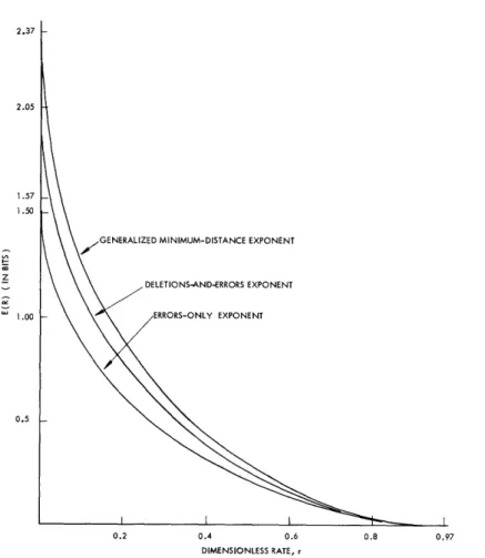
GENERALIZED MINIMUM-DISTANCE EXPONENT
17
EXPONENT
0.2 0.4 0.6
DIMENSIONLESS RATE, r
Fig. 3. Minimum-distance decoding exponents for a Gaussian
channel with L = 3. 23 2.37 2.05 1.57 1.50 t Q, 1.00 0.5 0.8 0.97 i
c. Computational Comparisons
To get some feeling for the relative performance of these three progressively more involved minimum-distance decoding schemes, the error exponents for each of them were computed over a few simple channels, with the use of the bounds discussed above.
In order to be able to compute easily the error-likelihood ratio, we considered only
channels with two inputs. Figure 3 displays a typical result; these curves are for a
channel with additive Gaussian noise of unit variance and a signal of amplitude either +3 or -3, which is a high signal-to-noise ratio. At lower signal-to-noise ratios the curves are closer. We also considered a two-dimensional Rayleigh fading channel for various signal-to-noise ratios.
For these channels, at least, we observed that though improvement is, of course, obtained in going from one decoding scheme to the next more complicated, this improve-ment is quite slight at high rates, and even at low rates, where improveimprove-ment is greatest, the exponent for generalized minimum-distance decoding is never greater than twice that
for errors-only decoding. The step between errors-only and deletions-and-errors
decoding is comparable to, and slightly greater than, the step between the latter and generalized minimum-distance decoding.
From these computations and some of the computations that will be reported in Sec-tion VI, it would seem that the use of deleSec-tions offers substantial improvements in per-formance only when very poor outputs (with error-likelihood ratios greater than one)
In Figure 5 by these rules we have constructed a chart of the first 5 powers of the
field elements. Observe that in every case P5 = [3, while with the exception of the zero
4
element V, P = I. Furthermore, both II and III have the property that their first four
powers are distinct, and therefore yield the 4 nonzero field elements. Therefore if we
o 4 3 2
let a denote the element II, say, I = a = a, II = a, III = a , and IV = a , which gives
us a convenient representation of the field elements for multiplication and division, in
log10 x
the same way that the logarithmic relationship x = U
sentation of the real numbers for multiplication and division.
P P2 P3 4 P5
P
~
pp
II III IV V I I IV III IV II I IV V V V II III IV V II II I IV Vgives us a convenient
repre-+ , -1
2 3
4
0 0
Fig. 5. Powers of the field elements. Fig. 6. Representations for GF(5).
Figure 6 displays the two representations of GF(5) that are convenient for addition
and multiplication. If p corresponds to a and ab, and y corresponds to c and a, then
p + y a + c mod 5, P- ¥=a - c mod 5, p. ¥ [ b + d m°a d 4 ] and py. -I
a
[b - d 4 ] a, an nd P
a[b-dmod4], where means 'corresponds to' and the 'mod 4' in the exponent arises,
4 o
since a = a = 1.
The prime field of most practical interest is GF(2), whose two elements are simply 0 and 1. Addition and multiplication tables for GF(2) appear in Fig. 7.
It can be shown2 1 that the general finite field GF(q) has q = pm elements, where p
is again a prime, called the characteristic of the field, and m is an arbitrary integer. As with GF(5), we find it possible to construct two representations of GF(q), one
con-venient for addition, one for multiplication. For addition, an element P of GF(q) is
represented by a sequence of m integers, bl,b 2,... ,bm. To add to a, we add b1
to c, b to c, and so forth, all modulo p.
0 1
1 1 0
0 1
00 0
10 1
Fig. 7. Tables for GF(2).
For multiplication, it is always possible to find a primitive element a, such that the first q - 1 powers of a yield the q - 1 nonzero field elements.
Thus aq - 1 = a = 1 (or else the first q - 1 powers would
not be distinct), and multiplication is accomplished by
adding exponents mod q - 1. We have, if is any
non-zero element, pq-1 (aa)q-1 = (aq-l)a = la = 1, and
thus for any , zero or not, pq = .
Thus all that remains to be specified is the proper-ties of GF(q) to make the one-to-one identification between the addition and multiplication
representations. Though this is easily done by using polynomials with coefficients from
26
-l
__
____III_1__LII___II 4---·YC- C·-l I_^l·l··^I1L----^-11-_1_1·-
·Ill-^lpll-
I
_ I
X ,
III. BOSE-CHAUDHURI-HOCQUENGHEM CODES
Our purpose now is to make the important class of BCH codes accessible to the reader with little previous background, and to do so with emphasis on the nonbinary BCH codes, particularly the RS codes, whose powerful properties are insufficiently known.
The presentation is quite single-minded in its omission of all but the essentials
needed to understand BCH codes. The reader who is interested in a more rounded
expo-sition is referred to the comprehensive and still timely book by Peterson.4 In particular,
our treatment of finite fields will be unsatisfactory to the reader who desires some depth
of understanding about the properties that we assert; Albert2 1 is a widely recommended
mathematical text. 3. 1 FINITE FIELDS
Mathematically, the finite field GF(q) consists of q elements that can be added,
sub-tracted, multiplied, and divided almost as numbers. There is always a field element
called zero (0), which has the property that any field element
P
plus or minus zero is P.There is also an element called one (1), such that P 1 = ; further, P 0 = 0. If is
not zero, it has a multiplicative inverse which is that unique field element satisfying the
equation p · P- 1 = 1; division by is accomplished by multiplication by P- 1
The simplest examples of finite fields are the integers modulo a prime number p. For instance, take p = 5; there are 5 elements in the field, which we shall write I, II,
III, IV, and V, to distinguish them from the integers to which they correspond.
Addi-tion, subtracAddi-tion, and multiplication are carried out by converting these numbers into
their integer equivalents and doing arithmetic modulo 5. For instance, I + III = IV,
since 1 + 3 = 4 mod 5; III + IV = II, since 3 + 4 = 2 mod 5; I III = III, since 1 · 3 = 3
mod 5; III IV = II, since 3 4 = Z mod 5. Figure 4 gives the complete addition and
multiplication tables for GF(5).
I II III IV V II III IV V I I III IV V I II I I IV V I II III III V I II III IV IV I II III IV V V I II III I V V I I III I I II IV V II IV I III V III I IV II V IV III I I I V V V V V V
ADDITION TABLE MULTIPLICATION TABLE
Fig. 4. Arithmetic in GF(5).
Note that V + = , if
P
is any member of the field; therefore, V must be the zeroelement. Also V P = V. I = P, so I must be the one element. Since I I = II III=
IV IVI, I- I, II-1 - -1 = IV.
IV.IV = I, I = I, II = III, III =II, and IV =IV.
I III IV V
GF(p),4, 21 it is not necessary to know precisely what this identification is to understand
the sequel. (In fact, avoiding this point is the essential simplification of our
presenta-tion.) We note only that the zero element must be represented by a sequence of m zeros.
As an example of the general finite field, we use GF(4) = GF(22), for which an addi-tion table, multiplicaaddi-tion table, and representaaddi-tion table are displayed in Fig. 8.
Note that GF(4) contains two elements that can be identified as the two elements of GF(2),
O 1 a b O 1 a b
0 0 0 0 010 0 b namely and 1. In this case GF(Z) is said to
1
1 0 b a 1 1 a b be a subfield of GF(4). In general, GF((q'))a a a b 0 I a b 1 a a 0 a b 0 b 1 is a subfield of GF(q) if and only if q = q,a
b ba 1 O b O b 1 a
where a is an integer. In particular, if q
ADDITION MULTIPLICATION m
p , the prime field GF(p) is a subfield of
+,- x, GF(q).
0 00 0 We shall need some explanation to
under-1 01 stand our later comments on shortened RS
a 10
b 11 codes. For addition, we have expressed the
REPRESENTATIONS elements of GF(q) as a sequence of m ele-ments from GF(p), and added place-by-place
Fig. 8. Tables for GF(4). according to the addition rules of GF(p), that
is, modulo p. Multiplication of an element
of GF(q) by some member b of the subfield GF(p) amounts to multiplication by an inte-ger b modulo p, which amounts to b-fold addition of the element of GF(q) to itself, which finally amounts to term-by-term multiplication of each of the m terms of the
ele-ment by b mod p. (It follows that multiplication of any element of GF(pm ) by p gives
a sequence of zeros, that is, the zero element of GF(pm).) It is perhaps plausible that
the following facts are true, as they are : if q = q'a, elements from GF(q) can always
be expressed as a sequence of b elements from GF(q'), so that addition of 2 elements from GF(q) can be carried out place-by-place according to the rules of addition in
GF(q'), and multiplication of an element from GF(q) by an element from GF(q') can
be carried out by term-by-term multiplication of each element in the sequence repre-senting GF(q) by P according to the rules of multiplication in GF(q').
As an example, we can write the elements of GF(16) as
00 10 aO a20
01 11 al a21
Oa la aa a2a
2 2 2 22
Oa la aa a a
where a is a primitive element of GF(4). Then, by using Fig. 5, (la) + (aa) = (a2 0), for
example, while a (al) = (a a).
27
We have observed that p = 0 for all elements in a field of characteristic p. In
particular, if p = 2, P + = 0, so that P = -P and addition is the same as subtraction
in a field characteristic two. Furthermore, (p+y)P = pP + (P) p 1 + ... + (pPl) yp1 +
yP, by the binomial theorem; but every term but the first and last are multiplied by p,
therefore zero, and (+y)P = pP + yP, when and y are elements of a field of
charac-teristic p.
3. 2 LINEAR CODES
We know from the coding theorem that codes containing an exponentially large num-ber of code words are required to achieve an exponentially low probability of error.
Linear codes4 ' 22 can contain such a great number of words, yet remain feasible to
gen-erate; they can facilitate minimum distance decoding, as we shall see. Finally, as a
class they can be shown to obey the coding theorem. They have therefore been
over-whelmingly the codes most studied.
Assume that we have a channel with q inputs, where q is a prime power, so that we can identify the different inputs with the elements of a finite field GF(q). A code word
f of length n for such a channel consists of a sequence of n elements from GF(q). We
shall write f = (fl,f 2,... fn) where fi occupies the ith place. The weight w(f) of f is
defined as the number of nonzero elements in f.
A linear combination of two words fl and f2 is written pfl + Yf2, where p and y are
each elements of GF(q), and ordinary vectorial (that is, place-by-place) addition in
GF(q) is implied. For example, if f = (fll'f1 2'f 13 ) and f2 = (f2 1'f 2 2'f23)' then
f1 f2 (fll -f2 1 f1 2-f 2 2'f 1 3-f 2 3).
A linear code of length n is a subset of the qn words of length n with the important property that any linear combination of words in the code yields another word in the code. A code is nondegenerate if all of its words are different; we consider only such codes.
Saying that the distance between two words f 1 and f2 is d is equivalent to saying that
the weight of their difference, w(fl-f2), is d, since fl - f2 will have zeros in places in
which and only in which the two words do not differ. In a linear code, moreover, fl -f
must be another code word f3, so that if there are two code words separated by
dis-tance d there is a code word of weight d, and vice versa. Excluding the all-zero,
zero-weight word, which must appear in every linear code, since 0 fl + 0 f2, is a valid
linear combination of code words, and the minimum distance of a linear code is then the minimum weight of any of its words.
We shall be interested in the properties of sets of j different places, or sets of
size j, which will be defined with reference to a given code. If the j places are such
that there is no code word but the all-zero word with zeros in all j places, we say that these j places form a non-null set of size j for that code; otherwise they form a null
set.
If there is a set of k places such that there is one and only one code word corre-sponding to each of the possible qk assignments of elements from GF(q) to those k places,