Detailed 2D flow simulations as an onset for evaluating socio-economic impacts of floods

1 INTRODUCTION

In the framework of the Belgian national research project “ADAPT - Towards an integrated decision tool for adaptation measures”, the hydraulic model WOLF 2D serves as a core component of a decision-support system (DSS). The tool is dedicated to the integrated evaluation of flood protection measures in the context of increased flood risk as a result of cli-mate change. This DSS takes into consideration hy-draulic, economic, social as well as environmental parameters to quantify flood risk.

Prior to assessing the effects of different flood protection measures, a preliminary step consists in determining how floodplain inundations and their socio-economic impacts are likely to be affected by climate change. Besides a comprehensive presenta-tion of the 2D hydraulic model and its validapresenta-tion, the present paper describes how the model is imple-mented in the framework of integrated flood risk as-sessment, with a focus on the selection of relevant climate change scenarios for hydraulic modelling and on the discussion of the simulation results for a specific case study located along the river Ourthe in the Meuse basin (Belgium).

The hydraulic model is based on the shallow-water equations solved by means of a finite volume technique. Multiblock Cartesian grids are exploited, enabling local mesh adaptation, while an automatic mesh refinement tool embedded in the hydraulic

model leads to significant reductions in computation time for simulating steady flows. Wetting and drying of computation cells is handled free of mass conser-vation error.

Consistently with the high resolution Digital Sur-face Model (airborne laser altimetry) used as topog-raphic data to represent the floodplains, computation grids as fine as 2m by 2m are used for the hydraulic simulations. Such spatial spacing is definitely fine enough to reproduce accurately the flow pattern at the building scale, as confirmed by several valida-tion examples based on comparisons between nu-merical predictions and measurements or observa-tions during past major flood events.

With the purpose of evaluating the impact of cli-mate change on floodplain inundations along river Ourthe, hydraulic modelling is conducted for four different climate change scenarios (perturbation fac-tors affecting peak discharges) and two different re-turn periods, likely to lead to complementary flood protection strategies. The four climate change sce-narios reflect the wide range of uncertainty affecting the discharge predictions deduced from results of re-gional climate modelling and hydrological model-ling, mainly as a result of the discrepancies in the various scenarios used for running the climate mod-els. The obtained hydraulic results (inundation ex-tent, pattern of water depth and flow velocity) serve as key input for the subsequent socio-economic and environmental assessment of flood risk.

Detailed 2D flow simulations as an onset for evaluating socio-economic

impacts of floods

B.J. Dewals

Research Unit of Hydrology, Applied Hydrodynamics and Hydraulic Constructions (HACH), Department ArGEnCo, University of Liege, Belgium & Postdoctoral Researcher of the Fund for Scientific Research, F.R.S.-FNRS, Belgium

S. Detrembleur, P. Archambeau, S. Erpicum & M. Pirotton

Research Unit of Hydrology, Applied Hydrodynamics and Hydraulic Constructions (HACH), Department ArGEnCo, University of Liege, Belgium

ABSTRACT: A 2D hydraulic numerical model is presented. It is based on the fully dynamic shallow-water equations, solved by means of a finite volume scheme on multiblock structured grids. The model handles highly accurate DSM derived from airborne laser altimetry for the floodplains and sonar detection for the bathymetry of the main channel. The flow simulations are performed with a typical grid spacing of 2m, com-parable to the resolution of the DSM and fine enough to represent reliably the flows at the scale of each build-ing. Consequently, the model succeeds in predicting accurately the pattern of flood depth even in densely ur-banized floodplains, as confirmed by several validation examples, which also demonstrate the ability of the model to reproduce depth measurements for a wide range of flood discharges without the need for recalibra-tion of the roughness coefficient. Finally, the hydraulic model is exploited as a component of a complete flood risk modelling chain, accounting for socio-economic and ecological impacts of floods and dedicated to the assessment of flood protection measures in the context of climate change.

2 HYDRODYNAMIC MODEL

As an onset for evaluating socio-economic impacts of floods, simulations of floodplain inundation flows are conducted with the numerical model WOLF 2D, developed at the University of Liege and based on a finite volume scheme.

2.1 Mathematical model

The model is based on the two-dimensional depth-averaged equations of volume and momentum con-servation, namely the “shallow-water” equations (SWE). In the “shallow-water” approach the basic assumption states that velocities normal to a main flow direction are smaller than those in the main flow direction. As a consequence the pressure field is found to be almost hydrostatic everywhere.

The large majority of flows occurring in rivers, even highly transient, can reasonably be seen as shallow everywhere, except in the vicinity of some singularities (e.g. weirs). Indeed, vertical velocity components remain generally low compared to ve-locity components in the horizontal plane and, con-sequently, flows may be considered as mainly two-dimensional. Therefore, the approach presented here may definitely be regarded as suitable for floodplain inundation modelling.

2.1.1 Conservation laws

The conservative form of the depth-averaged equa-tions of volume and momentum conservation can be written as follows, using vector notations

d d 0 f t x y x y ∂ ∂ ∂ ₊∂ ₊∂ _{+ + = −} ∂ ∂ ∂ ∂ ∂ f g s f g S S , (1)

with s = [h hu hv]T the vector of the conservative unknowns. f and g represent the advective and pres-sure fluxes in directions x and y, while. fd and gd are the diffusive fluxes:

2 1 2 2 hu hu gh huv ⎛ ⎞ ⎜ ⎟ =_⎜ + _⎟ ⎜ ⎟ ⎝ ⎠ f , _d 0 x xy h _σ ρ τ ⎛ ⎞ ⎜ ⎟ = − ⎜ ⎟ ⎜ ⎟ ⎝ ⎠ f , (2) 2 1 2 2 hv huv hv gh ⎛ ⎞ ⎜ ⎟ = ⎜ ⎟ ⎜ ₊ ⎟ ⎝ ⎠ g , 0 xy y h _τ ρ σ ⎛ ⎞ ⎜ ⎟ = − ⎜ ⎟ ⎜ ⎟ ⎝ ⎠ g . (3)

S0 and Sf designates respectively the bottom slope term and the friction term:

[

]

T 0 = −gh 0 ∂zb ∂x ∂zb ∂y S , (4) T f = ⎣⎡0 τ ρ τbx by ρ⎤⎦ S . (5)

The following notations have been used: t = time; x and y = space coordinates; h = water depth, u and

v = depth-averaged velocity components, zb =bottom elevation, g = gravity acceleration, ρ = density of water, τbx and τby = bottom shear stresses, σx and

σy = turbulent normal stresses, and τxy = turbulent shear stress.

2.1.2 Closure relations: friction and turbulence The bottom friction is conventionally modelled thanks to an empirical law, such as the Manning formula. The model enables the definition of a spa-tially distributed roughness coefficient. Besides, the friction along side walls is reproduced by means of a process-oriented formulation (Dewals 2006):

2 2 2 2 b b w 4 / 3 1/ 3 1 4 , 3 x x N x k n u n u u v gh h h y τ ρ = ⎡ ⎤ = _⎢ + + _⎥ Δ ⎣

∑

⎦ (6) 2 3/ 2 b 2 2 b w 4 / 3 1/ 3 1 4 , 3 y y N y k n v n v u v gh h h x τ ρ = ⎡ ⎤ = ⎢ + + ⎥ Δ ⎢ ⎥ ⎣

∑

⎦ (7)

where the Manning coefficients nb and nw (s/m1/3) characterize respectively the bottom and the side-walls roughness. Those relations are particularized for Cartesian grids, as exploited in the present study.

The internal friction may be accounted for thansk to the turbulence model included in WOLF 2D. The turbulent stresses are expressed following the Bous-sineq approximation (transposed for a depth-averaged model) (ASCE Task Committee on Turbu-lence Models in Hydraulic Computations 1988; Rodi 1984):

(

T

)

2 x u x σ _{ν ν} ρ ∂ = + ∂ , 2

(

T

)

y v y σ ν ν ρ ∂ = + ∂ , (8)

(

T

)

xy yx u v y x τ τ ν ν ρ ρ ∂ ∂ ⎛ ₊ ⎞ = = + _{⎜ ⎟} ∂ ∂ ⎝ ⎠, (9)

where ν = molecular kinematic viscosity, νΤ = eddy voscosity computed by a turbulence closure model (ν اν_Τ).

For this purpose, two different approaches are available in WOLF 2D:

− first, a simple algebraic turbulence closure, as-suming that the turbulence is bed-dominated, leading to the following expression for the turbu-lent kinematic: ν_T =αhu_*, with α taking values

of the order 0.5 (Fischer et al. 1979);

− second, an original depth-averaged k-ε model with two different length-scales accounting for vertical and horizontal turbulence mixing, as de-veloped by Erpicum (Erpicum 2006).

Nevertheless, for the present computations, no tur-bulence model has been activated. All friction ef-fects are thus globalized in the bottom and wall fric-tion terms.

2.2 Computational implementation 2.2.1 Space discretization

The computation domain is discretized by means of a multiblock grid, in which each consists in a locally Cartesian mesh. Since this multiblock structure en-ables refined meshes close to interesting areas, it compensates for the usual drawbacks of Cartesian grids, while keeping the benefits of structured grids in terms of accuracy and computation time.

The space discretization of the divergence form of the 2D conservative shallow-water equations is performed by means of a finite volume scheme. For the applications considered in this study, this ap-proach warranties that the numerical model is free from mass and momentum conservation errors.

Within each block, variable reconstruction at cells interfaces can be performed by constant or linear ex-trapolation, in conjunction with a slope limiter, lead-ing respectively to a first or second order accuracy. Variables at the border between adjacent blocks are extrapolated linearly, using additional ghost points as depicted in Figure 1. The value of the variables at the ghost points is evaluated from the value of the subjacent cells. Moreover, to ensure conservation properties at the border between adjacent blocks and thus to compute accurate volume and momentum balances, fluxes related to the larger cells are com-puted at the level of the finer ones.

Appropriate flux computation has always been a challenging issue in computational fluid dynamics. In the present study, fluxes f and g are computed by a Flux Vector Splitting (FVS) method developed by the authors. According to this FVS, the upwinding direction of each term of the fluxes f and g is simply dictated by the sign of the flow velocity recon-structed at the cells interfaces. It has thus the advan-tage of being completely Froude independent and of facilitating a satisfactory adequacy with the discreti-zation of the bed elevation gradient (Erpicum 2006).

Figure 1. Evaluation of fluxes at the interface between two ad-jacent blocks on the Cartesian multiblock grid.

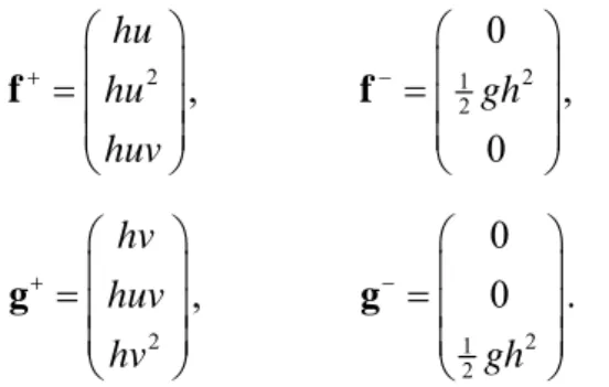
The FVS can be formally expressed as follows:

2 hu hu huv + ⎛ ⎞ ⎜ ⎟ = ⎜ ⎟ ⎜ ⎟ ⎝ ⎠ f , 1₂ 2 0 0 gh − ⎛ ⎞ ⎜ ⎟ = ⎜ ⎟ ⎜ ⎟ ⎝ ⎠ f , (10) 2 hv huv hv + ⎛ ⎞ ⎜ ⎟ = ⎜ ⎟ ⎜ ⎟ ⎝ ⎠ g , 2 1 2 0 0 gh − ⎛ ⎞ ⎜ ⎟ = ⎜ ⎟ ⎜ ⎟ ⎝ ⎠ g . (11)

where the exponents + and − refer to, respectively, an upstream and a downstream evaluation of the cor-responding terms. A Von Neumann stability analysis has demonstrated that this FVS leads to a stable spa-tial discretization of the terms ∂f/∂x and ∂g/∂y in Equation 1 (Dewals 2006).

This FVS has already proved its validity and effi-ciency for numerous applications (Archambeau et al. 2004; Dewals 2006; Dewals et al. 2006a, 2006b; Dewals et al. 2008b; Erpicum 2006; Erpicum et al. 2008). Due to their diffusive nature, the fluxes fd and

gd are legitimately evaluated by means of a centred scheme.

2.2.2 Time discretization

Since the model is applied to compute steady-state solutions, the time integration is performed by means of a three-step first order accurate Runge-Kutta algorithm, providing adequate dissipation in time. For stability reasons, the time step is con-strained by the Courant–Friedrichs–Levy (CFL) condition based on gravity waves. A semi-implicit treatment of the bottom friction term (3) is used, without requiring additional computational costs. 2.2.3 Boundary conditions

The value of the specific discharge is prescribed as an inflow boundary condition. Besides, the trans-verse specific discharge is set to zero at the inflow. The outflow boundary condition may be a prescribed water surface elevation, a Froude number or no con-dition in case of supercritical outflow. At solid walls, the component of the specific discharge nor-mal to the wall is set to zero. For the purpose of evaluating the diffusive terms, the gradients of the unknowns must also be specified at the boundaries. These gradients in the direction parallel to the boundary are set to zero for simplicity, while the gradients of the variables in the direction normal to the boundary are properly evaluated by finite differ-ence between the value at the boundary and the value at the centre of the next cell (Erpicum 2006). 2.2.4 Mesh adaptation and automatic refinement A grid adaptation technique is used to restrict the computation domain to the wet cells and a narrow strip surrounding the wet cells. The grid is thus adapted at each time.

a b c

a' b' c'

Ghost point Domain boundary Flux evaluation

As a result of an iterative resolution of the conti-nuity equation prior to the evaluation of the momen-tum equations, wetting and drying of computation cells is handled free of volume and momentum con-servation errors (Erpicum 2006).

In addition, the model includes an automatic

mesh refinement algorithm (AMR). For steady-state

simulations, the AMR tool consists in performing the computation on several successive grids, starting from a very coarse one and gradually refining it up to the finest one. When the hydrodynamic fields are stabilized on one grid, the solver automatically jumps onto a finer one. The successive solutions are interpolated from the coarser towards the finer grid. This fully automatic method considerably reduces the number of cells in the first grids and thus sub-stantially decreases the total computation time, de-spite slight extra computation time required for meshing and interpolation operations (section 7.4). 2.3 The modelling system WOLF

The herein described model constitutes a part of the modelling system “WOLF”, developed at the Uni-versity of Liege. WOLF includes a set of comple-mentary and interconnected modules for simulating free surface flows: process-oriented hydrology, 1D & 2D hydrodynamics, sediment (Dewals 2006) or pollutant transport, air entrainment, as well as an op-timisation tool based on Genetic Algorithms (Er-picum 2006).

Other functionalities of WOLF 2D include the use of moment of momentum equations (Dewals 2006), the application of the cut-cell method (Er-picum 2006), as well as computations considering bottom curvature effects by means of curvilinear co-ordinates in the vertical plane (Dewals 2006; Dewals et al. 2006a).

A user-friendly interface, entirely designed and implemented by the authors (Archambeau 2006), makes the pre- and post-processing operations very convenient. Import and export operations are easily feasible from and to various classical GIS tools. Several layers of maps can be handled to facilitate the analysis of various data sets such as topography, ground characteristics, vegetation density, hydrody-namic fields...

3 TOPOGRAPHIC DATA

For about a decade, high resolution, high accuracy topographic datasets have become increasingly available for inundation modelling in a number of countries. In Belgium, a data collection programme using airborne laser altimetry (LIDAR) has gener-ated high quality topographic data covering the floodplains of most rivers in the southern part of the country. Simultaneously, the bathymetry of the main

rivers has been surveyed by means of an echo-sonar technique.

Consequently, combining the data generated from those two remote sensing techniques enables to ob-tain a complete Digital Surface Model (DSM) char-acterized by a horizontal resolution of 1 m by 1 m and with a vertical accuracy of 15 cm. As regards smaller non navigable rivers, cross sections are properly interpolated to generate a two-dimensional bathymetry.

Those high quality topographic data combined with simulations performed on grids as fine as 2 m by 2 m enable to set the value of roughness coeffi-cients to represent only small scale roughness ele-ments and not to globalize larger scale effects such as blockage by buildings or by large irregularities of the topography. It enables also to conduct inundation modelling at the scale of each house and street indi-vidually.

Nevertheless, since inundation flows may be ex-tremely sensitive to some local topographic charac-teristics, such as for instance the exact height of a protection wall, a crucial step consists in validating and enhancing the DSM by removing residual obsta-cles non relevant for the flow (e.g. vegetation), by integrating additional sources of topographic data (including field survey) as well as the detailed ge-ometry of flood protections and other hydraulic structures (weirs, water intakes …). The large amount of data collected from those various sources is stored into an efficient database structure.

4 PROCEDURE FOR INUNDATION

MODELLING IN THE SOUTH OF BELGIUM Since 2003, the flow model WOLF 2D has been ap-plied to conduct inundation modeling along over 800 km of the main rivers in the southern part of Belgium 800 km. A 4-step modeling procedure has been elaborated and applied systematically for each river reach:

1 elaboration from laser altimetry and sonar data (or cross sections) of the complete DSM (main riverbed and floodplains) with a grid resolution of 1 m by 1 m,

2 validation and enhancement of the DSM by a field survey and the integration of additional geometric characteristics,

3 flow modelling of past flood events with the pur-pose of calibrating and validating the roughness parameters,

4 Computation of the inundation maps for constant statistical flood discharge values with a 25-, 50- and 100-year return period.

Depending on the river width, the flow modelling steps 3 and 4 are conducted with a grid spacing varying between 1 m and 5 m, with a typical value of 2 m.

5 STEADY-STATE ASSUMPTION

All the simulations detailed in the rest of the present paper refer to river reaches located in the sub-basin of river Meuse situated in Belgium.

As detailed by de Wit et al. (2007), the Meuse ba-sin covers an area of about 33,000 km2, including parts of France, Luxembourg, Belgium, Germany and the Netherlands. It can be subdivided into three major geological zones, referred to as “Lotharingian Meuse” (southern part), “Ardennes Meuse” (central part) and the Dutch and Flemish lowlands (northern part).

While the southern and northern parts are charac-terized by wide floodplains where flood waves are significantly attenuated, in the central part of the Meuse basin, between Charleville-Mézières and Liège, the Meuse is captured in the Ardennes massif, characterized by narrow steep valleys, where flood waves are hardly attenuated.

The rivers considered hereafter are all situated in the central part of the Meuse basin. As shown in Figure 2, the tributaries of river Meuse which flow in the Ardennes Massif present the largest river gra-dients (de Wit et al. 2007). Consequently, the flood waves along this type of rivers are hardly attenuated as a result of the combination of the steep gradients and of the relatively narrow cross-sectional shape of the valleys (de Wit et al. 2007), leading to very low storage capacity in the floodplains. As a result the floodplains are completely filled with water quickly after the beginning of the flood and a quasi-steady flow is then observed.

For instance, for typical floods occurring on the river Ourthe, it has been verified that the volume of water stored in the inundated floodplains along a 10 km-long reach remains lower than one percent of the total amount of water brought by the flood wave. Therefore, the steady-state assumption has been considered as valid for simulating floodplain inunda-tion along most rivers of the Ardennes Massif and is systematically used in the simulations discussed in the subsequent paragraphs. An additional benefit of this assumption is reduced run time as a result of the possibility to exploit automatic mesh refinement.

Figure 2. River gradients of Meuse and its tributaries. Adapted from de Wit et al. (2007) and Berger (1992).

Besides, comparisons have been made between inundation patterns predicted by unsteady flow simulations, for which the real flood hydrograph is prescribed as an upstream boundary condition, and inundation patterns computed assuming a steady-state flow (constant discharge close to the peak dis-charge of the hydrograph). Those comparisons have confirmed that the maximum flood extents predicted by the two approaches are in very good agreement.

6 VALIDATION OF INUNDATION MODELLING

The inundation model has been slightly calibrated (roughness coefficient) and subsequently validated by comparison of the numerical results with ob-served flood extents and measured water depths dur-ing recent floods events. Reference data were ob-tained at gauging stations, collected by field surveys or deduced from aerial pictures of the flood.

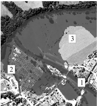
Figure 3. Aerial photography of the inundation pattern along a meandering reach of the river Lesse on January 28th_{, 1995}

(peak discharge: 180 m³/s).

Figure 4. Simulated inundation extent along a meandering reach of the river Lesse for the flood of January 28th, 1995 (peak discharge: 180 m³/s).

6.1 Example 1: inundation pattern along river

Lesse

Located in the south-east of Belgium, the 89 km-long river Lesse is a tributary of the River Meuse and has a catchment area of 1343 km2 _{(mean annual} discharge: 19 m3/s at his mouth into river Meuse). Figure 3 and Figure 4 compare the inundation extent along a meandering reach of the river for the flood which occurred on January 28th, 1995. The peak dis-charge is evaluated at 180 m³/s, corresponding to a return period of 15 years. As shown by the reference points 1, 2 and 3 (Figs. 2 and 3), the predicted spa-tial pattern of inundation, simulated with a grid spac-ing of 2 m in the riverbed and 4 m in the floodplains, is found to match observations very well.

6.2 Example 2: water profile along the river

Amblève

River Amblève springs in the eastern part of Bel-gium, close to the border with Germany, and flows towards the west into river Ourthe. It is 80 km long, has a mean discharge of 19.5 m3_{/s at his mouth and} the catchment areas covers 1077 km2.

During a flood in December 1993 (discharge: 300 m3/s, return period: 10-15 years), water surface elevations have been measured at 11 locations along the most downstream reach of the river.

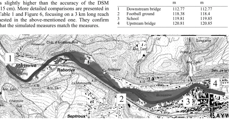
Comparisons between this set of data and the predictions of the numerical model (grid spacing: 2 m everywhere) show a satisfactory agreement, with an absolute not exceeding 11 cm along the 12 km long considered reach (Figure 5). It must be emphasized that a single calibrated value of the roughness coefficient has been use for the whole length of the channel and that the achieved accuracy is slightly higher than the accuracy of the DSM (15 cm). More detailed comparisons are presented in Table 1 and Figure 6, focusing on a 3 km long reach nested in the above-mentioned one. They confirm that the simulated measures match the measures.

6.3 Example 3: rating curve along river Vesdre River Vesdre is also a tributary of river Ourthe. It is 70 km long, with a mean discharge of 12 m3/s at his mouth and a catchment area of 700 km2.

Figure 7 displays the measured stage-discharge relationship as well as 6 additional points obtained from numerical simulation of a XX km long reach. Figure 7 shows that the numerical model succeeds in predicting the water depth in the main riverbed for a wide range of discharges (150-300 m3/s). The simu-lations for the six discharge values have been per-formed with the same roughness coefficient, show-ing that no recalibration is necessary as far as water depths in the main channel are considered.

Figure 5. Measured vs. simulated free surface elevation along a reach of the river Amblève during the 1993-flood (300 m³/s). Table 1. Comparison between observed and simulated water surface elevations at some selected places along the river Am-blève for the flood of Decembre 21st_{, 1993.}

___________________________________________________

Location Measured Simulated

m m ___________________________________________________ 1 Downstream bridge 112.77 112.77 2 Football ground 118.38 118.4 3 School 119.81 119.85 4 Upstream bridge 120.81 120.85 ___________________________________________________

Figure 6. Inundation extent simulated for the flood of December 21st_{, 1993 along a 3 km long reach of the river Amblève}

(dis-charge: 298 m³/s). The numbers refer to the location of the four points for which water surface elevations are compared in Table 1.

-0.1 -0.05 0 0.05 0.1 0.15 0.2 0.25 95 100 105 110 115 120 125 130 0 2000 4000 6000 8000 10000 12000 Er ro r ( m ) F ree s ur fa ce el ev at io n (m )

Length along the channel(m) Error

Simulated Measured

Figure 7. Measured vs. simulated free surface elevation for

dif-ferent discharges along the river Vesdre. Figure 8. Measured vs. simulated free surface elevation for dif-ferent discharges along the river Vesdre.

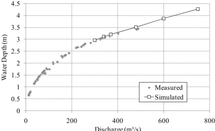
6.4 Example 2: rating curve along the river Semois Finally, a similar comparison is shown for the river Semois (Figure 8), which is a 210 km long tributary of the river Meuse and has a catchment area of 1350 km2 (mean discharge: 35 m3/s at his mouth). Again, the simulated water depths have been suc-cessfully validated for discharge values ranging be-tween 300 m3/s and 500 m3/s, without recalibration of the roughness coefficient. The hydraulic model has next been applied to extend the stage-discharge curve towards more extreme discharge values in the range 500-800 m3/s (Figure 8).

7 INUNDATION MODELLING AS AN ONSET FOR EVALUATING SOCIO-ECONOMIC IMPACTS OF FLOODS CONSIDERING CLIMATE CHANGE

7.1 Flood risk modelling approach and elaboration

of a Decision Support System (DSS)

In the framework of the Belgian national research project “ADAPT - Towards an integrated decision tool for adaptation measures”, the 2D hydraulic model serves as a core component of a decision-support system dedicated to the integrated evalua-tion of flood protecevalua-tion measures in the context of an expected increase in flood risk as a result of climate change. This tool is based on a combination of cost-benefit analysis (CBA) and multi-criteria analysis (MCA), taking into consideration hydraulic, eco-nomic, social and ecological indicators for character-izing flood risk.

More details on damage evaluation and flood risk quantification are provided in a companion paper (Dewals et al. 2008a). In contrast, the following paragraphs concentrate on how the 2D hydraulic model is implemented within the system, with a fo-cus on the selection of modelling scenarios, on the efficiency of different computation procedures and on the simulation results.

7.2 Case study and preliminary steps

In order demonstrate the efficiency of the decision-support system and to facilitate its refinement, the methodology is first tested on a case study, which covers two neighbouring reaches of the lower Our-the river in Our-the Meuse basin. This 20 km-long mean-dering part of river Ourthe, between the municipali-ties of Poulseur and Tilff is situated a few kilometres upstream of the mouth of river Ourthe into the Meuse river.

Prior to evaluating the benefits of different adap-tation measures, a preliminary step consists in de-termining how inundation hazard is likely to be modified by climate change. More precisely, for floods of different return periods and for several climate change scenarios, 2D hydraulic simulations are run in order to identify which modifications cli-mate change will cause to inundation extents as well as water depths and flow velocities in the flood-plains.

7.3 Climate change scenarios

Results of Global Circulation Models (GCM) and Regional Climate Models (RCM) provide estimates of the potential increase in precipitation (winter and spring) and potential changes in evapotranspiration as a result of climate change. Those predicted changes are affected by a significant level of uncer-tainty due to the climate models themselves and, to an even greater extent, due to the discrepancies in the scenarios used for running those climate models (Intergovernmental Panel on Climate Change 2007).

Moreover, translating those changes in precipita-tion and evapotranspiraprecipita-tion into changes in river dis-charges is also a challenging task, since the catch-ment response depends on many factors such as the land roughness and permeability, the rainfall dura-tion, … Therefore, at the present stage of the ADAPT project, simple assumptions have been con-sidered regarding the expected changes in the peak

78 78.5 79 79.5 80 80.5 81 81.5 82 0 50 100 150 200 250 300 F ree s ur fa ce e lev at io n ( m ) Discharge (m³/s) Measured Simulated 0 0.5 1 1.5 2 2.5 3 3.5 4 4.5 0 200 400 600 800 Wa te r D ep th (m ) Discharge (m³/s) Measured Simulated

discharges of river Ourthe as a result of climate change. Indeed, according to a comprehensive litera-ture review (De Groof et al. 2006; Dewals et al. 2007), an increase by 10% of flood discharge may be regarded as reasonable. Moreover, in order to evaluate the sensitivity of the results with respect to this perturbation factor on the discharge, increases by 5% and by 15% have also been considered. Be-sides, a more extreme case has been simulated as well (+30%), consistently with the wide ranges of uncertainties affecting the results of GCM and RCM. All those assumptions will eventually be con-firmed and refined by comparison with the output of a hydrological model (De Groof et al. 2006).

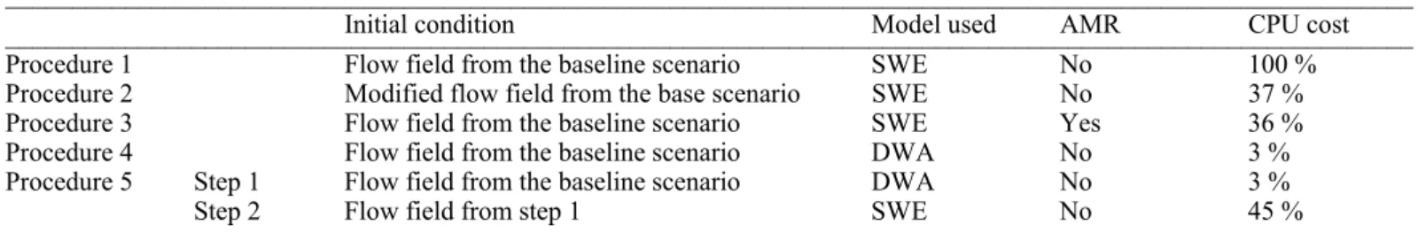
7.4 Most efficient computation procedure

The computation time is an issue of primary impor-tance because of the need for repeated runs both for predicting the impact on floodplain inundations of different climate change scenarios and, for evaluat-ing as well as optimizevaluat-ing a number of adaptation measures. Therefore, comparisons have been made between different procedures, which differ by the initial condition considered, by the optional use of a simplified hydraulic model as a preconditioning, or by the optional exploitation of Automatic Mesh Re-finement (AMR). In the tests mentioned hereafter and involving AMR, the following grid sizes have been used sequentially: 32m, 16m, 8m, 4m and 2m.

The different procedures compared are detailed in Table 2 for the case of computing the flow for a spe-cific climate change scenario. In procedure 2, the modified initial condition refers to an a priori in-crease in the initial water depth by a constant value in the whole domain (this value may be estimated for instance from the change in the downstream boundary condition or from a uniform flow calcula-tion for the updated discharge ...).

In Procedure 5, the Diffusive Wave

Approxima-tion (DWA) is used as a precondiApproxima-tioning for the

SWE model. In contrast with the fully dynamic SWE, the DWA approach assumes that the advec-tive terms of the SWE may be neglected. In such a case, the free surface slope is only balanced by the friction term. Ad hoc computational schemes for solving the DWA model have been detailed by Ar-chambeau et al. (2004) and ArAr-chambeau (2006).

Al-though remaining nonlinear (through the friction law), the DWA model requires significantly less computation time. For that reason, the DWA ap-proach is exploited to performs a first quick compu-tation of an approximate solution, which is next in-troduced as an “enhanced” initial condition for the SWE model.

Table 2 also provides the relative computation time necessary for the different procedures to con-verge towards a steady state solution, compared to Procedure 1. For comparison purpose, procedure 4 provides the computation time required if only the DWA is exploited. This strategy appears to be by far the most efficient one. However inaccuracies in the water depth and flow velocity patterns are found as a consequence of the simplifying assumptions lying under the DWA approach. Those inaccuracies reach up to 50 cm locally in terms of water depth, which is unacceptable compared to the expected changes in-duced by climate change and limiting the computa-tion to the DWA is hence considered as not accept-able in the case of the present analysis.

Similarly, the overall efficiency of procedure 5 appears disappointing as a result of too big inaccura-cies obtained at the end of step 1 (DWA), which prevent a very fast convergence of step 2 (SWE). Therefore, procedure 3, which involves the AMR technique (§ 2.2.4) and is shown to the second fast-est one, is presently identified as the most efficient one for performing repeated steady-state simula-tions, preserving the full accuracy of the SWE. 7.5 Results of inundation modelling

Table 3 summarizes the different hydraulic simu-lations performed for the two considered reaches of the river Ourthe. It also provides averaged values of the change in water depths; while detailed results are available in the form of updated inundation maps in-dicating, for each return period and each climate change scenario, the two-dimensional pattern of wa-ter depth, flow velocity in the floodplains. This set of results serves as an input for the subsequent dam-age evaluation and flood risk assessment, conducted by means of corresponding modules of the decision-support system.

Table 2. Relative run time necessary for the different computation procedures to provide a steady state solution.

__________________________________________________________________________________________________________

Initial condition Model used AMR CPU cost

__________________________________________________________________________________________________________ Procedure 1 Flow field from the baseline scenario SWE No 100 %

Procedure 2 Modified flow field from the base scenario SWE No 37 % Procedure 3 Flow field from the baseline scenario SWE Yes 36 % Procedure 4 Flow field from the baseline scenario DWA No 3 % Procedure 5 Step 1 Flow field from the baseline scenario DWA No 3 %

Step 2 Flow field from step 1 SWE No 45 %

Table 3. Updated discharges and average change in water depth induced by Climate Change (CC) for two different return periods along the two considered reaches of river Ourthe.

__________________________________________________________________________________________________________ Baseline CC scenario CC scenario CC scenario CC scenario scenario n°1 (+5%) n°2 (+10%) n°3 (+15%) n°4 (+30%) __________________________________________________________________________________________________________ Discharge 726 m3_{/s 762 m}3_{/s 799 m}3_{/s 835 m}3_{/s 944 m}3_/s

25-year flood Reach n°1 - + 10 cm + 25 cm + 40 cm + 75 cm

Reach n°2 - + 10 cm + 25 cm + 40 cm + 70 cm

__________________________________________________________________________________________________________ Discharge 876 m3_{/s 920 m}3_{/s 964 m}3_{/s 1007 m}3_{/s 1139 m}3_/s

100-year flood Reach n°1 - + 15 cm + 30 cm + 45 cm + 75 cm

Reach n°2 - + 20 cm + 40 cm + 60 cm + 85 cm

__________________________________________________________________________________________________________

As shown in Table 3, it is found that the results can be very sensitive to the perturbation factor af-fecting the discharge, due for instance to the reduced efficiency of flood protection structures (e.g. dikes) above a threshold value of discharge (design dis-charge).

7.6 Hydrodynamic modelling of flood protection

measures

The hydraulic model is next applied to simulate the hydraulic effect of various local flood protection measures along river Ourthe and to demonstrate their potential efficiency in spite of the relatively limited storage capacity of the floodplains. In con-trast, due to the narrow shape of the valley and the relatively long duration of the floods in this lower part of the Ourthe catchment, standard flood control areas have no chance to protect population and goods from inundation by damping the flood wave, since such areas would be completely filled with wa-ter long before the flood peak is reached. Therefore, the main riverbed and its floodplains must be de-signed to enable the flood discharge to flow through the most vulnerable localities without causing dam-aging overflows.

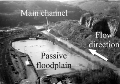
The herein described example of flood protection measure consists in transforming non-urbanized

pas-sive floodplains into active ones. “Paspas-sive”

flood-plain refers to an inundation area in which flow ve-locity remain extremely small (Figure 9). As shown in Figure 10 and 11, the activation of a passive floodplain consists in modifying the topography to enable the development of higher flow velocities be-yond in the floodplain. As a result, the effective width (and thus section) of the river is increased and, consequently, the water level upstream is reduced (by 50 cm in the example shown in Figure 11).

Figure 9. Passive floodplain along the river Ourthe during the flood of February 2002.

Figure 10. Initial topography and velocity field (100 year-flood, CC scenario n°2) in the considered reach of river Ourthe, before activation of the floodplain. The location of topography changes and the effective flow widths are highlighted.

Figure 11. Modified topography and velocity field (100 year-flood, CC scenario n°2) along the considered reach of river Ourthe after activation of the floodplain. The location of topog-raphy changes and the effective flow widths are highlighted.

8 CONCLUSION

An advanced 2D hydraulic numerical model has been presented. It is based on the fully dynamic shallow-water equations, solved by means of a finite volume scheme on multiblock structured grids. The model also incorporates an automatic mesh refine-ment tool. The only calibration parameter is the roughness coefficient, which can be spatially dis-tributed both in the main riverbed and in the flood-plains.

The model handles routinely highly accurate DSM derived from airborne laser altimetry for the floodplains and sonar detection for the bathymetry of the main channel. For river reaches as long as 10 to 15km, the flow simulation may be performed with a grid spacing of 2m, comparable to the resolution of the DSM and fine enough to represent reliably the flows at the scale of each building individually.

Consequently, the model succeeds in predicting accurately the local pattern of flood depth, as con-firmed by several validation examples detailed in the paper. The validation demonstrates the ability of the model to predict the inundation extent and to repro-duce depth measurements for a wide range of flood discharges without the need for recalibration. The model also offers the potential to represent the ve-locity pattern even in densely urbanized floodplains. Finally, the hydraulic model is exploited as a component of a complete flood risk modelling chain dedicated to the assessment of flood protection measures in the context of climate change. Analysis of climate change effect on floodplain inundation has been detailed for a case study along river Ourthe (Meuse basin).

Since such an analysis requires repeated runs of the hydraulic model, both for evaluating a number of climate change scenarios and next for assessing the hydraulic effect of various flood protection meas-ures, comparisons between different computations strategies have been undertaken and have revealed that the automatic mesh refinement technique proves to enhance considerably the convergence rate to-wards a steady flow.

9 ACKNWOLEDGEMENT

Part of this work has been carried out on behalf of the Belgian Science Policy (BELSPO), in the framework of the research program “Science for a Sustainable Development”.

The authors also gratefully acknowledge the Wal-loon Ministry of Facilities and Transport (MET-SETHY) for the fruitful collaboration and for the provided data sets (including topographic data).

10 REFERENCES

Archambeau, P. 2006. Contribution à la modélisation de la

ge-nèse et de la propagation des crues et inondations:

Univer-sity of Liege. PhD thesis: 423.

Archambeau, P., B. Dewals, S. Detrembleur, S. Erpicum & M. Pirotton. 2004. A set of efficient numerical tools for flood-plain modeling. Shallow Flows. G. H. Jirka & W. S. J. Uijt-tewaal. Leiden, etc: Balkema: 549-557.

ASCE Task Committee on Turbulence Models in Hydraulic Computations. 1988. Turbulence modeling of surface water flow and transport: Part I. J. Hydraul. Eng.-ASCE 114(9): 970-991.

Berger, H. E. J. 1992. Flow forecasting for the river Meuse: Delft University of Technology. PhD thesis.

De Groof, A., W. Hecq, I. Coninx, K. Bachus, B. Dewals, M. Pirotton, M. El Kahloun, P. Meire, L. De Smet & R. De Sutter. 2006. General study and evaluation of potential

im-pacts of climate change in Belgium - Research report.

de Wit, M. J. M., H. A. Peeters, P. H. Gastaud, P. Dewil, K. Maeghe & J. Baumgart. 2007. Floods in the Meuse basin: event descriptions and an international view on ongoing measures. Intl. J. River Basin Management 5(4): 279-292. Dewals, B. 2006. Une approche unifiée pour la modélisation

d'écoulements à surface libre, de leur effet érosif sur une structure et de leur interaction avec divers constituants:

University of Liege. PhD thesis: 636.

Dewals, B. J., R. De Sutter, L. De Smet & M. Pirotton. 2007. Synthesis of primary impacts of climate change in Belgium, as an onset to the development of an assessment tool for adaptation measures. Geophysical Research Abstracts

9(11217).

Dewals, B. J., J. Ernst, S. Detrembleur, P. Archambeau, S. Er-picum & M. Pirotton. 2008a. Integration of accurate 2D inundation modelling, vector land use database and econo-mic damage evaluation. Proc. European Conference on

Flood Risk Management - FloodRisk 2008. Balkema.

Dewals, B. J., S. Erpicum, P. Archambeau, S. Detrembleur & M. Pirotton. 2006a. Depth-integrated flow modelling taking into account bottom curvature. J. Hydraul. Res. 44(6): 787. Dewals, B. J., S. Erpicum, P. Archambeau, S. Detrembleur &

M. Pirotton. 2006b. Numerical tools for dam break risk as-sessment: validation and application to a large complex of dams. Improvements in reservoir construction, operation

and maintenance. H. Hewlett. London: Thomas Telford.

Dewals, B. J., S. A. Kantoush, S. Erpicum, M. Pirotton & A. J. Schleiss. 2008b. Experimental and numerical analysis of flow instabilities in rectangular shallow basins. Environ.

Fluid Mech. 8: 31-54.

Erpicum, S. 2006. Optimisation objective de paramètres en

écoulements turbulents à surface libre sur maillage multi-bloc: University of Liege. PhD thesis: 356.

Erpicum, S., P. Archambeau, S. Detrembleur, B. Dewals & M. Pirotton. 2008. A 2D finite volume multiblock flow solver applied to flood extension forecasting. Numerical modelling

of hydrodynamics for water ressources. P. García-Navarro

& E. Playán. London: Taylor & Francis: 321-325.

Fischer, H. B., E. J. List, R. C. Y. Koh, J. Imberger & N. H. Brooks. 1979. Velocity Distribution in Turbulent Shear Flow. Mixing in Inland and Coastal Waters.

Intergovernmental Panel on Climate Change. 2007. Climate change 2007: Synthesis Report.

Rodi, W. 1984. Turbulence models and their application in