O
pen
A
rchive
T
OULOUSE
A
rchive
O
uverte (
OATAO
)
OATAO is an open access repository that collects the work of Toulouse researchers and
makes it freely available over the web where possible.
This is an author-deposited version published in :
http://oatao.univ-toulouse.fr/
Eprints ID : 15295
The contribution was presented at TENOR 2015 :
http://tenor2015.tenor-conference.org/
To cite this version : Gu
yot, Patrice and Pinquier, Julien Browsing soundscapes.
(2015) In: 1st International Conference on Technologies for Music Notation and
Representation (TENOR 2015), 28 May 2015 - 30 May 2015 (Paris, France).
Any correspondence concerning this service should be sent to the repository
administrator:
[email protected]
BROWSING SOUNDSCAPES
Patrice Guyot SAMoVA team - IRIT University of Toulouse - France [email protected]
Julien Pinquier SAMoVA team - IRIT University of Toulouse - France [email protected]
ABSTRACT
Browsing soundscapes and sound databases generally re-lies on signal waveform representations, or on more or less informative textual metadata. The TM-chart representation is an efficient alternative designed to preview and compare soundscapes. However, its use is constrained and limited by the need for human annotation. In this paper, we de-scribe a new approach to compute charts from sounds, that we call SamoCharts. SamoCharts are inspired by TM-charts, but can be computed without a human annotation. We present two methods for SamoChart computation. The first one is based on a segmentation of the signal from a set of predefined sound events. The second one is based on the confidence score of the detection algorithms. SamoCharts provide a compact and efficient representation of sounds and soundscapes, which can be used in different kinds of applications. We describe two application cases based on field recording corpora.
1. INTRODUCTION
Compact graphical representations of sounds facilitate their characterization. Indeed, images provide instantaneous vi-sual feedback while listening sounds is constrained by their temporal dimension. As a trivial example, record cov-ers allow the user to quickly identify an item in a collec-tion. Such compact representation is an efficient means for sound identification, classification and selection.
In the case of online databases, the choice of a sound file in a corpus can be assimilated to the action of browsing. As proposed by Hjørland, “Browsing is a quick examination of the relevance of a number of objects which may or may not lead to a closer examination or acquisition/selection of (some of) these objects” [1].
Numerous websites propose free or charged sound file downloads. These files generally contain sound effects,
Copyright: 2015 Patrice Guyot et al.c This is an open-access article distributed under the terms of the Creative Commons
Attribution Licence 3.0 Unported, which permits unre-stricted use, distribution, and reproduction in any medium, provided the original author and source are credited.
isolated sound events, or field recordings. Applications are numerous, for instance for music, movie soundtracks, video games and software production. In the context of the CIESS project1, our work focuses on an urban sound
database used for experimental psychology research. Most of the times, on-line access to sound files and data-bases is based on tags and textual metadata. These meta-data are generally composed of a few words description of the recording, to which may be added the name of its au-thor, a picture of the waveform, and other technical proper-ties. They inform about the sound sources, recording con-ditions or abstract concepts related to the sound contents (for example “Halloween”).
Natural sonic environments, also called field recordings or soundscapes [2], are typically composed of multiples sound sources. Such audio files are longer than isolated sound events, usually lasting more than one minute. There-fore, short textual descriptions are very hard to produce, which makes it difficult to browse and select sounds in a corpus.
The analysis and characterization of urban sound events has been reported in different studies. Notably, they can be merged in identified categories [3], which leads to a tax-onomical categorization of environmental sounds (see [4] for an exhaustive review). Outdoor recordings are often composed of the same kinds of sound sources, for instance
birds, human voices, vehicles, footstep, alarm, etc. There-fore, the differences between two urban soundscapes (for example, a park and a street) mostly concern the time of presence and the intensity of such identified sources. As a consequence, browsing field recordings based on the known characteristics of a set of predetermined sound events can be an effective solution for their description.
Music is also made of repeated sound events. In instru-mental music, these events can be the notes, chords, clus-ters, themes and melodies played by the performers. When electroacoustic effects or tape music parts come into play, they can be of a more abstract nature. In the case of musique
concrete, the notion of “sound object” (which in practice is generally a real sound recording) has its full meaning and
1http://www.irit.fr/recherches/SAMOVA/
a central position in the music formalization itself [5]. As long as events are identified though, we can assume that the previous soundscape-oriented considerations hold for musical audio files as well.
The TM-chart [6] is a tool recently developed to provide compact soundscape representations starting from a set of sound events. This representation constitutes a bridge be-tween physical measures and categorization, including acous-tic and semanacous-tic information. Nevertheless, the creation of a TM-chart relies on manual annotation, which is a tedious and time-consuming task. Hence, the use of TM-charts in the context of big data sets or for online browsing applica-tions seems unthinkable.
Besides sound visualization, automatic annotation of au-dio recordings recently made significant progress. The gen-eral public has recently witnessed the gengen-eralization of speech recognition system. Significant results and efficient tools have also been developed in the fields of Music Informa-tion Retrieval (MIR) and Acoustic Event DetecInforma-tion (AED) in environmental sounds [7], which leads us to reckon with sustainable AED in the coming years.
In this paper, we propose a new paradigm for soundscape representation and browsing based on the automatic iden-tification of predefined sounds events. We present a new approach to create compact representations of sounds and soundscapes that we call SamoCharts. Inspired by TM-Charts and recent AED techniques, these representations can be efficiently applied for browsing sound databases. In the next section we present a state of the art of online sound representations. The TM-chart tool is then described in Section 3, and Section 4 proposes a quick review of Audio Event Detection algorithms. Then we present in Section 5 the process of SamoCharts creation, and some applications with field recordings in Section 6.
2. SOUND REPRESENTATION 2.1 Temporal Representations
From the acoustic point of view, the simplest and predom-inant representation of a sound is the temporal waveform, which describes the evolution of sound energy over time. Another widely used tool in sound analysis and represen-tation is the spectrogram, which shows more precisely the evolution of the amplitude of frequencies over time. How-ever, spectrograms remain little used by the general public. While music notation for instrumental music has focused on the traditional score representation, the contemporary and electro-acoustic music communities have introduced alternative symbolic representation tools for sounds such as the Acousmograph [8], and the use of multimodal infor-mation has allowed developing novel user interfaces [9].
All these temporal representations are more or less in-formative depending on the evolution of the sound upon the considered duration. In particular, in the case of field recordings, they are often barely informative.
2.2 Browsing Sound Databases
On a majority of specialized websites, browsing sounds is based on textual metadata. For instance, freeSFX2 clas-sifies the sounds by categories and subcategories, such as
public placesand town/city ambience. In a given subcate-gory, each sound is only described with a few words text. Therefore, listening is still required to select a particular recording.
Other websites, such as the Freesound project,3 add a waveform display to the sound description. In the case of short sound events, this waveform can be very informative. On this website it is colored according to the spectral cen-troid of the sound, which adds some spectral information to the image. However, this mapping is not precisely de-scribed, and remains more aesthetic than useful.
The possibility of browsing sounds with audio thumbnail-ing has been discussed in [10]. In this study, the authors present a method for searching structural redundancy like the chorus in popular music. However, to our knowledge, this kind of representation has not been used in online sys-tems so far.
More specific user needs have been recently observed through the DIADEMS project4 in the context of audio
archives indexing. Through the online platform Telemeta5,
this project allows ethnomusicologists to visualize specific acoustic information besides waveform and recording meta-data, such as audio descriptors and semantic labels. This information aims at supporting the exploration of a corpus as well as the analysis of the recording. This website il-lustrates how automatic annotation can help to index and organize audio files. Improving its visualization could help to assess the similarity of a set of songs, or to underline the structural form of the singing turns by displaying homoge-neous segments.
Nevertheless, texts and waveforms remain the most used and widespread tools on websites. In the next sections, we present novel alternative tools, that have been specially designed for field recording representation.
2http://www.freesfx.co.uk/ 3https://www.freesound.org/
4http://www.irit.fr/recherches/SAMOVA/DIADEMS/ 5http://telemeta.org/
3. TM-CHART 3.1 Overview
The Time-component Matrix Chart (abbreviated TM-chart) was introduced by Kozo Hiramatsu and al. [6]. Based on a <Sound Source × Sound level> representation, this chart provides a simple visual illustration of a sonic environment recording, highlighting the temporal and energetic pres-ence of sound sources. Starting from a predetermined set of sound events (e.g. vehicles, etc.), and after preliminary annotation of the recording, the TM-chart displays percent-ages of time of audibility and percentpercent-ages of time of level ranges for the different sound sources. They constitute ef-fective tools to compare sonic environment (for instance daytime versus nighttime recordings).
3.2 Method
Despite a growing bibliography [11, 12], the processing steps involved in the creation of TM-charts as not been pre-cisely explained. We describe in this part our understand-ing of these steps and our approach to create a TM-chart.
3.2.1 Estimation of the Predominant Sound
TM-charts rely on a preliminary manual annotation, which estimates the predominant sound source at each time. To perform this task, the signal can be divided in short seg-ments, for example segments of one second. For each segment, the annotator indicates the predominant sound source. This indication is a judgment that relies on both the loudness and the number of occurrences of the sources. An example of annotation can be seen on Figure 1.
Afterwards, each segment label is associated to a cate-gory of sound event, which can be for instance one of car,
voice, birds, or miscellaneous.
Figure 1. Preliminary annotation of a sound recording for the creation for the creation of a TM-chart.
3.2.2 Computation of the Energy Level
An automatic process is applied to compute the energy of the signal and the mean energy of each segment (respec-tively in blue and red curves on Figure 1). We assume that the sound pressure level can be calculated from the record-ing conditions with a calibrated dB meter.
In this process, we can notice that the sound level of a segment is not exactly the sound level of its predominant source. Indeed the sound level of an excerpt depends upon the level of each sound sources, and not only the predom-inant one. However, we assume that these two measures are fairly correlated.
3.2.3 Creation of the TM-chart
We can now calculate the total duration in the recording (in terms of predominance) and the main sound levels for each category of sound. From this information, a TM-chart can be created.
Figure 2 shows a TM-chart based on the example from Figure 1. It represents, for each category of sound, the percentage of time and energy in the soundscape. The ab-scissa axis shows the percentage of predominance for each source in the recording. For one source, the ordinate axis shows the duration of its different sound levels. For exam-ple, the car-horn is audibly dominant for over 5 % of time. Over this duration, the sound level of this event exceeds 60 dB for over 80 % of time.
Figure 2. Example of a TM-chart.
3.2.4 Interpretation of the TM-chart
Charts like the one on Figure 2 permit quick interpreta-tions of the nature of the sound events that compose a soundscape. We could infer for instance that the sound-scape has been recorded close to a little traffic road, with distant conversations (low energy levels). From such inter-pretation, one can clearly distinguish and compare sonic environments recorded in different places [6].
The main issue in the TM-chart approach is the need for manual annotation, a time-consuming operation which cannot be applied to big data sets. Therefore, the use of TM-charts seems currently restricted to specific scientific research on soundscapes. In the next sections we will show how recent researches and works on sound analysis can be leveraged to overcome this drawback.
4. AUDIO EVENT DETECTION
Various methods have been proposed for the Audio Event Detection (AED) from continuous audio sequences recorded in real life. These methods can be divided in two cate-gories.
The first category of methods aims at detecting a large set of possible sound events in various contexts. For in-stance, the detection of 61 types of sound, such as bus
door, footsteps or applause, has been reported in [7]. In this work the author modeled each sound class by a Hidden Markov Model (HMM) with 3 states, and Mel-Frequency Cepstral Coefficients (MFCC) features. Evaluation cam-paigns, such as CLEAR [13] or AASP [14], propose the evaluation of various detection methods on a large set of audio recordings from real life.
The second category of methods aims at detecting fewer specific types of sound events. This approach privileges accuracy over the number of sounds that can be detected. It generally relies on a specific modeling of the “target sounds” to detect, based on acoustic observations. For ex-ample, some studies propose to detect gunshots [15] or wa-ter sounds [16], or the presence of speech [17].
These different methods output a segmentation of the sig-nal informed by predetermined sound events. They can also provide further information that may be useful for the representation, particularly in the cases where they are not reliable enough. Indeed, the detection algorithms are generally based on a confidence score, that allows to tune the decisions. For instance, Hidden Markov Model, Gaus-sian mixture models (GMM) or Support Vector Machine (SVM), all rely on confidence or “likelihood” values. Since temporal confidence values can be computed by each method of detection, it is possible to output at each time the proba-bility that a given sound event is present in the audio signal. Based on these observations, we propose a new tool for soundscape visualization, the SamoChart, which can rely either on automatic sound event segmentation, or on confi-dence scores by sound events.
5. SAMOCHART
The SamoChart provides a visualization sound recordings close to that of a chart. At the difference of a TM-chart, it can be computed automatically from a segmenta-tion or from temporal confidence values.
In comparison with TM-charts, the use of the automatic method overcomes a costly human annotation and avoids subjective decision-making.
5.1 Samochart based on Event Segmentation
5.1.1 Audio Event Segmentation
SamoCharts can be created from Audio Event Detection annotations. This automatic annotation is an independent process that can be performed following different approaches, as mentioned in Section 4. We will suppose in the next part that an automatic annotation has been computed from a set of potential sound events (“targets”). For each target sound event, this annotation provides time markers related to the presence or absence of this sound in the overall record-ing. In addition to the initial set of target sounds, we add a sound unknown that corresponds to the segments that have not been labeled by the algorithms.
5.1.2 Energy Computation
As in the TM-chart creation process, we compute the en-ergy of the signal. However, if the recording conditions of the audio signal are unknown, we cannot retrieve the sound pressure level. In this case, we use the RMS energy of each segment, following the equation:
RM S(w) = 20 × log10 v u u t N X i=0 w2(i) (1) where w is an audio segment of N samples, and w(i) the value of the ith
sample.
5.1.3 SamoChart Creation
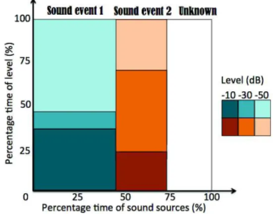
From the information of duration and energy, we are able to create a SamoChart. Figure 3 shows an example of a SamoChart based on event segmentation considering two possible sound events.
Figure 3. SamoChart based on event segmentation.
Unlike TM-charts, we can notice from this method that the total percentage of sound sources can be higher than 100% if the sources overlap.
5.2 Samochart based on Confidence Values
Most Audio Event Detection algorithms actually provide more information than the output segmentation. In the following approach, we propose to compute SamoCharts from the confidence scores of these algorithms.
We use for each target sound the temporal confidence val-ues outputted by the method, which can be considered as probabilities of presence (between 0 and 1). The curve on Figure 4 shows the evolution of the confidence for the pres-ence of a given sound event during the analyzed recording. We use a threshold on this curve, to decide if the sound event is considered detected or not. This threshold is fixed depending on the detection method and on the target sound. To obtain different confidence measures, we divide the up-per threshold portion in different parts.
Figure 4. Confidence measures for a sound event.
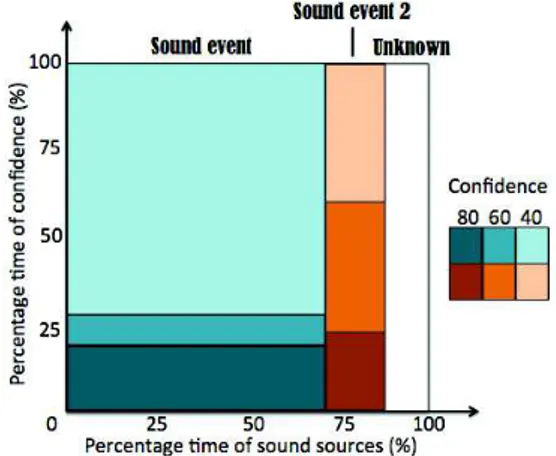
With this approach, we infer the probability of presence for each sound event according to a confidence score. Fig-ure 5 shows the SamoChart associated to a unique sound event. In this new chart, the sound level is replaced by the confidence score.
Figure 5. SamoChart based on confidence value.
5.3 Implementation
We made a JavaScript implementation to create and dis-play SamoCharts, which performs a fast and “on the fly”
computation of the SamoChart. The code is downloadable from the SAMoVA web site6. It uses an object-oriented paradigm to facilitate future development.
In order to facilitate browsing applications, we also chose to modify the size of the chart according to the duration of the corresponding sound excerpt. We use the equation 2 to calculate the height h of the Samochart from a duration d in seconds. h= 1 if d <1 2 if1 ≤ d < 10 2 × log10(d) if d ≥10 (2)
We also implemented a magnifying glass function that provides a global view on the corpus with the possibility of zooming in into a set of SamoCharts. Furthermore, the user can hear each audio file by clinking on the plotted charts.
6. APPLICATIONS
6.1 Comparison of soundscapes (CIESS project) Through the CIESS project, we have recorded several ur-ban soundscapes at different places and times. The sound events of these recordings are globally the same, for in-stance vehicle and footstep. However, their numbers of oc-currences are very different according to the time and place of recording. As an application case, we computed sev-eral representations of two soundscapes. Figure 6 shows the colored waveforms of these extracts as they could have been displayed on the Freesound website.
Figure 6. Colored waveforms of two soundscapes.
As we can see, these waveforms do not show great differ-ences between the two recordings.
We used AED algorithms to detect motor vehicle, foot-step and car-horn sounds on these two example record-ings [18]. Then, we computed SamoCharts based on the confidence score of these algorithms (see Figure 7).
The SamoCharts of Figure 7 are obviously different. They provide a semantic interpretation of the soundscapes, which reveals important dissimilarities. For instance, the vehicles are much more present in the first recording than in the second one. Indeed, the first recording was recorded on an important street, while the second one was recorded on a pedestrian street.
6http://www.irit.fr/recherches/SAMOVA/
Figure 7. SamoCharts of the two recordings of Figure 6, based on confi-dence values.
6.2 Browsing a corpus from the UrbanSound project If the differences between two soundscapes can easily be seen by comparing two charts, the main interest of the SamoChart is their computation on bigger sound databases. UrbanSound dataset7 has been created specifically for
soundscapes research. It provides a corpus of sounds that are labeled with the start and end times of sound events of ten classes: air conditioner, car horn, children playing,
dog bark, drilling, enginge idling, gun shot, jackhammer, sirenand street music. The SamoCharts created from these annotations allow to figure out the sources of each file, as well as their duration and their sound level. They give an overview of this corpus. Figure 8 shows the SamoCharts of nine files which all contain the source car horn. The duration of these files range form 0.75 to 144 seconds.
Figure 8. Browsing recordings of the UrbanSound corpus.
6.3 SoundMaps
Other applications can be found from the iconic chart of a soundscape. Soundmaps, for example, are digital ge-ographical maps that put emphasis on the soundscape of every specific location. Various projects of sound maps
7https://serv.cusp.nyu.edu/projects/
urbansounddataset/
have been proposed in the last decade (see [19] for a re-view). Their goals are various, from giving people a new way to look at the world around, to preserving the sound-scape of specific places. However, as in general with sound databases, the way sounds are displayed on the map is usu-ally not informative. The use of SamoCharts on soundmaps can facilitate browsing and make the map more instructive. 6.4 Music Representations
If the process we described to make charts from sounds was originally set up to display soundscapes, it could cer-tainly be extended to other contexts. Indeed, Samocharts give an instantaneous feedback on the material that com-pose the sonic environment. Handled with the appropri-ate sound cappropri-ategories, they could provide a new approach to overview and analyze a set of musical pieces composed with the same material.
For example, Samocharts could be used on a set of con-crete music pieces. The charts could reveal the global uti-lization of defined categories of sounds (such as bell or
birds songs). In the context of instrumental music analysis, they could reflect the utilization of the different families of instrument (e.g. brass, etc.), representing the duration and musical nuances. Applied on a set of musical pieces or ex-tracts, they could emphasize orchestration characteristics.
Figure 9 shows an analysis of the first melody (Theme A) of Ravel’s Bol´ero, which is repeated nine times with dif-ferent orchestrations. The SamoCharts on the figure dis-play orchestration differences, as well as the rising of a crescendo. The main chart (Theme A-whole) shows how each family of instrument is used during the whole extract.
Figure 9. Analysis of the first melody of Ravel’s Bol´erol (repetitions number 1, 4 and 9, and global analysis). The horizontal axis corresponds to the percentage of time where a family of instrument is present. This percentage is divided by the number of instruments: the total reaches 100% only if all instruments play all the time. The vertical axis displays the percentage of time an instrument is played in the different nuances.
7. CONCLUSION AND FUTURE WORKS In this paper, we presented a new approach to create charts for sound visualization. This representation, that we name SamoChart, is based on the TM-chart representation. Un-like TM-charts, the computation of SamoCharts does not rely on human annotation. SamoCharts can be created from Audio Event Detection algorithms and computed on big sound databases.
A first kind of SamoChart simply uses the automatic seg-mentation of the signal from a set of predefined sound sources. To prevent eventual inaccuracies in the segmen-tation, we proposed a second approach based on the confi-dence scores of the previous methods.
We tested the SamoCharts with two different sound data-bases. In comparison with other representations, Samo-Charts provide great facility of browsing. On the one hand, they constitute a precise comparison tool for soundscapes. On the other hand, they allow to figure out what kinds of soundscapes compose a corpus.
We also assume that the wide availability of SamoCharts would make them even more efficient for accustomed users. In this regard, we could define a fixed set of color which would correspond to each target sound.
The concepts behind TM-charts and Samocharts can fi-nally be generalized to other kind of sonic environments, for example with music analysis and browsing.
Acknowledgments
This work is supported by a grant from Agence Nationale de la Recherche with reference ANR-12-CORP-0013, within the CIESS project.
8. REFERENCES
[1] B. Hjørland, “The importance of theories of knowl-edge: Browsing as an example,” Journal of the
Amer-ican Society for Information Science and Technology, vol. 62, no. 3, pp. 594–603, 2011.
[2] R. Schafer and R. Murray, The tuning of the world. Knopf New York, 1977.
[3] C. Guastavino, “Categorization of environmental sounds.” Canadian Journal of Experimental
Psychol-ogy/Revue canadienne de psychologie exp´erimentale, vol. 61, no. 1, p. 54, 2007.
[4] S. Payne, W. Davies, and M. Adams, “Research into the practical and policy applications of soundscape concepts and techniques in urban areas,” University of
Salford, 2009.
[5] P. Schaeffer, Trait´e des objets musicaux. Paris: Edi-tions du Seuil, 1966.
[6] K. Hiramatsu, T. Matsui, S. Furukawa, and I. Uchiyama, “The physcial expression of sound-scape: An investigation by means of time component matrix chart,” in INTER-NOISE and NOISE-CON
Congress and Conference Proceedings, vol. 2008, no. 5. Institute of Noise Control Engineering, 2008, pp. 4231–4236.
[7] A. Mesaros, T. Heittola, A. Eronen, and T. Virtanen, “Acoustic event detection in real life recordings,” in
Proceedings of the 18th European Signal Processing Conference, 2010, pp. 1267–1271.
[8] Y. Geslin and A. Lefevre, “Sound and musical repre-sentation: the acousmographe software,” in
Proceed-ings of the International Computer Music Conference, 2004.
[9] D. Damm, C. Fremerey, F. Kurth, M. M¨uller, and M. Clausen, “Multimodal presentation and browsing of music,” in Proceedings of the 10th international
con-ference on Multimodal interfaces. ACM, 2008, pp. 205–208.
[10] M. A. Bartsch and G. H. Wakefield, “Audio thumbnail-ing of popular music usthumbnail-ing chroma-based representa-tions,” Multimedia, IEEE Transactions on, vol. 7, no. 1, pp. 96–104, 2005.
[11] T. Matsui, S. Furukawa, T. Takashima, I. Uchiyama, and K. Hiramatsu, “Timecomponent matrix chart as a tool for designing sonic environment having a diversity of sound sources,” in Proceedings of Euronoise, 2009, pp. 3658–3667.
[12] E. Bild, M. Coler, and H. W¨ortche, “Habitats assen pilot: Testing methods for exploring the correlation between sound, morphology and behavior,” in
Pro-ceedings of Measuring Behavior, M. W.-F. A.J. Spink, L.W.S. Loijens and L. Noldus, Eds., 2014.
[13] R. Stiefelhagen, K. Bernardin, R. Bowers, J. Garofolo, D. Mostefa, and P. Soundararajan, “The CLEAR 2006 evaluation,” in Multimodal Technologies for Perception
of Humans. Springer, 2007, pp. 1–44.
[14] D. Giannoulis, E. Benetos, D. Stowell, M. Rossignol, M. Lagrange, and M. Plumbley, “Detection and classi-fication of acoustic scenes and events,” An IEEE AASP
Challenge, 2013.
[15] C. Clavel, T. Ehrette, and G. Richard, “Events detec-tion for an audio-based surveillance system,” in
Pro-ceedings of the International Conference on Multime-dia and Expo, ICME. IEEE, 2005, pp. 1306–1309.
[16] P. Guyot, J. Pinquier, and R. Andr´e-Obrecht, “Wa-ter sound recognition based on physical models,” in
Proceedings of the 38th International Conference on Acoustics, Speech, and Signal Processing, ICASSP. IEEE, 2013.
[17] J. Pinquier, J.-L. Rouas, and R. Andr´e-Obrect, “Robust speech/music classification in audio documents,”
En-tropy, vol. 1, no. 2, p. 3, 2002.
[18] P. Guyot and J. Pinquier, “Soundscape visualization: a new approach based on automatic annotation and samocharts,” in Proceedings of the 10th European
Congress and Exposition on Noise Control Engineer-ing, EURONOISE, 2015.
[19] J. Waldock, “Soundmapping. critiques and reflections on this new publicly engaging medium,” Journal of