Structural Analysis in Differential-Algebraic Systems
and Combinatorial Optimization
?Mathieu Lacroix
1♦, A. Ridha Mahjoub
2, S´ebastien Martin
21LIMOS, Universit´e Blaise Pascal Clermont-Ferrand II, Complexe Scientifique des C´ezeaux,
63177 Aubi`ere Cedex, France ([email protected])
2LAMSADE, Universit´e Paris Dauphine, Place du Mar´echal De Lattre De Tassigny, 75775 Paris Cedex 16, France
([email protected]), ([email protected]) ABSTRACT
In this paper we consider the structural analysis problem for differential-algebraic systems with conditional equations. This problem consists, given a conditional differential algebraic system, in verifying if the system is well-constrained for every state, and if not to find a state in which the system is bad-constrained. We give a formulation for this problem as an integer linear program. This is based on a transformation of the problem to a matching problem in an auxiliary graph. We also show that the linear relaxation of that formulation can be solved in polynomial time. Using this, we develop a branch-and-cut algorithm for solving the problem.
Keywords: Differential algebraic system, structural analysis, graph, integer program, matching, branch-and-cut.
1. Introduction
Differential-algebraic systems (DAS) are used for model-ing complex physical systems as electrical networks and dynamic mouvements. Such a system can be given as
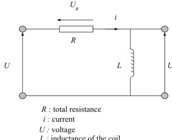
F (x, ˙x, u, p, t) = 0 (1) where x is the variable vector, u is the input vector, p is the parameter vector and t is time. As example, consider for instance the electrical circuit RL of Figure 1. This network contains a coil L and a resistance R in series. The voltage
U and current i at the terminal of the self are unknown.
Fig. 1: Electrical circuit.
For this circuit we can associate the following differential system : di dt = U L, 978-1-4244-4136-5/09/$25.00 2009 IEEE
?Supported by the project ANR-06-TLOG-26-01 PARADE ♦Current address: LAMSADE, Universit´e Paris Dauphine, Place du
Mar´echal De Lattre De Tassigny, 75775 Paris Cedex 16, France
E(t) = U + Ri,
where E(t) is a time function.
Establishing that a DAS definitely is not solvable can be helpful. A necessary (but not sufficient) criteria for solv-ability is that the number of variables and equations must agree. Object-oriented modeling langages like Modelica [5] enforce this as simulation is not possible if this is not the case. Thus before solving a DAS, it is utile to verify if there are as many equations as variables, and if there ex-ists a mapping between the equations and the variables in such a way that each equation is related to only one variable and each variable is related to only one equation. If this is satisfied, then we say that the system is well-constrained. Otherwise, the system is said to be constrained. A bad-constrained system is also refered as structurally singular
system. The structural analysis problem (SAP) of a DAS
consists in verifying if the system is well-constrained. The structural analysis problem has been considered in the literature for nonconditional DASs. In [10, 11], Murota develops a graph theoretical method for the structural anal-ysis of a system of equations. He introduces a formula-tion of the problem in terms of bipartite graphs, and shows that a system of equations is well-constrained if and only if there exists a perfect matching in the corresponding bipar-tite graph. He also introduces graph decomposition tech-niques that permit to identify the well and bad-constrained subsystems. This reduces to decomposing the associated graph into strong connected components. Such a decompo-sition can also be realized using the well known Dulmage and Mendelsohn decomposition [3]. Murota also studied extensions of his approach and further aspects within the framework of matroids and matrices. In [14], Reibig and Feldmann propose a structural method for solving DASs of the form
F (x, ˙x) = f (t). (2)
which are generated from the description of electrical net-works. The method is based on graph and matroid theory. It permits to reduce the problem to the determination of
which is called a fundamental circuit of a matroid, induced by a certain bipartite graph. Jian-Wan et al [7] and Nilsson [13] consider the SAP in relation with Modelica models. A Modelica source code is first translated into a so-called ”flat model” which is a system of equations of type 1. In [7], the authors propose a method for analysing and de-tecting minimal bad-constrained subsystems. The method uses Dulmage et Mendelsohn decomposition techniques in a first step to isolate the bad-constrained subsets of equa-tions. Then for each such subsystem, a set of fictitious equations is formulated. These are related to the underlay-ing physical system. The resultunderlay-ing system of equations is in turn decomposed and so on until a minimal bad-constrained subsystem is detected. The method is applied in a recursive way until all the minimal bad-constrained components are localized. In [13], the author studies the SAP for modular systems of equations, that is systems which are constructed by composition of individual equation system fragments. Leitold and Hangos [8] consider the DAS for dynamic pro-cess models. These are DAS which are sometimes diffi-cult to solve numerically due to index problems [1]. They propose a graph-theoretical method for analysing the dif-ferential index and the structural solvability of these mod-els. The method is an extension of Murota’s approach [10], where a representation graph is considered for each differ-ential index.
To the best of our knowledge, the SAP has not been con-sidered for DAS with conditional equations. This paper is concerned with this extension of the problem. The pur-pose of the paper is to propur-pose a model and a resolution approach for the problem in this case.
The paper is organized as follows. In Section 2, we dis-cuss the relation between DAS and matchings. In Section 3, we give a graph representation of SAP for conditional DAS. An integer programming formulation is proposed in Section 4. A polynomial time algorithm for solving the linear relaxation of this formulation is discussed in Section 5. And in Sections 6 and 7, we study an extension of our approach to DAS with embedded conditions.
2. Differential algebraic systems and matchings A matching of a graph is a subset of edges such that no two edges share a common node. Matchings have shown to be useful for modeling various discrete structures [9]. A well known and widely studied problem in combinatorial optimization is the matching problem. this consists, given a graph G = (V, E), in finding a matching with maximum cardinality [9],[4]. A graph is called bipartite if the ver-tices can be divided into two disjoint sets U and V such that every edge connects a node in U to one in V , that is,
U and V are independent sets. A matching M of a
bipar-tite graph G = (U ∪ V, E) such that |U | = |V | = n is called perfect if |M | = n. As mentioned above, the struc-tural analysis of a DAS is a first and necessary step before analysing the system by simulating. The aim of this step is to find out whether the system is well-constrained. Given a DAS, one can associate a bipartite graph G = (U ∪ V, E) where U corresponds to the equations, V to the variables, and there is an edge uivi ∈ E between a node ui ∈ U and a node vi ∈ V if the variable corresponding to vi appears in the equation corresponding to ui. Graph G is
called incidence graph. Therefore checking if the system is well-constrained can be realized by calculating a per-fect matching in the associated incidence graph. If such a matching does not exist, then the underlaying DAS is bad-constrained [10].
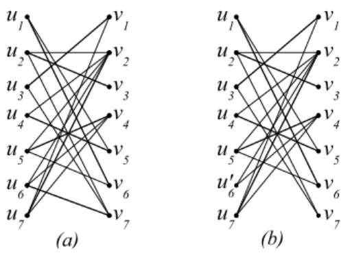
Consider, for instance, the following DAS :
eq1: 0 = x + 4y, eq2: 0 = 2u + z + ˙v, eq3: 0 = 3a + 3z + ˙z, eq4: 0 = x + 4u, (3) eq5: 0 = 2w + v + ˙y, eq6: 0 = 3w + 3u + ˙z, eq7: 0 = 3a + 3u + ˙w.
Let (3’) be the DAS obtained from (3) by replacing the equation eq6by the equation :
eq0
6: 0 = 3x + 3u
The incidence graphs corresponding to DAS (3) and (3’) are shown in Figure 2 (a) and (b), respectively. Here nodes u1, ..., u6, u06, u7 are associated with
equa-tions eq1, ..., eq6, eq06, eq7 and nodes v1, ..., v7 are
associ-ated with variables a, u, v, w, x, y, z, respectively. A per-fect matching is displayed in bold edges in Figure 2 (a), implying that system (3) is well-constrained. However, the maximum matching of the incidence graph corresponding to system (3’), displayed in Figure 2 (b), is not perfect, which implies that system (3’) is bad-constrained.
For more details on the relation between simple (noncon-ditional) DASs and matchings see [10, 11].
Fig. 2: Incidence graphs.
3. The SAP for conditional DAS
In many practical situations, physical systems have differ-ent states generated by some technical conditions. These may be, for instance, related to temperature changements in hydraulic systems. These physical systems generally yield DASs with conditional equations. Each conditional equation can generate several equations. In this section we discuss the SAP for these more general DASs. We will suppose, without loss of generality, that the conditional equations of the system all generate the same number of equations, for each combination of conditions. Otherwise,
the system would be bad-constrained. One can easily de-tect a conditional equation yielding less or more variables than equations, if there is any. Moreover we will suppose that each conditional equation may generate only one equa-tion. If this is not the case then one can expand the system to a one satisfying this. In fact, if a conditional equation
eqcond generates k equations with respect to a condition
cond, then it can be expanded to k conditional equations eq1, ..., eqk such that each equation eqi may generate the
ith equation of eq
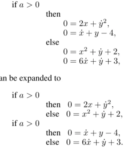
condaccording to condition cond whether it is true or false. For example the conditional equation
if a > 0 then 0 = 2x + ˙y2, 0 = ˙x + y − 4, else 0 = x2+ ˙y + 2, 0 = 6 ˙x + ˙y + 3, can be expanded to if a > 0 then 0 = 2x + ˙y2, else 0 = x2+ ˙y + 2, if a > 0 then 0 = ˙x + y − 4, else 0 = 6 ˙x + ˙y + 3.
A conditional DAS may then have different forms depend-ing on the set of conditions that hold each assignment. Here we consider conditional DAS such that any condi-tional equation may take two possible values, depending on whether the associated condition is true or false and may generate only one equation. The equations generated by a conditional equation will be refered as simple equation. Each assignment of the values true and false to the condi-tions yield a nonconditional system, called a state of the system.
Consider for example the following DAS:
eq1: if a > 0 then 0 = 4x2+ 2 ˙x + 4y + 2, else 0 = ˙y + 2z + 4, eq2: if b > 0 then 0 = 6 ˙y + 2 ˙z + 2, (4) else 0 = x + ˙y + 1, eq3: if c > 0 then 0 = 6 ˙x + y + 2, else 0 = 3 ˙y + z + 3.
For conditions a > 0, b > 0, c > 0, system (4) is nothing but the following.
eq1: 0 = 4x2+ 2 ˙x + 4y + 2,
eq2: 0 = 6 ˙y + 2 ˙z + 2, (5)
eq3: 0 = 6 ˙x + y + 2.
And conditions a > 0, b > 0, c ≤ 0 yield the system.
eq1: 0 = 4x2+ 2 ˙x + 4y + 2,
eq2: 0 = 6 ˙y + 2 ˙z + 2, (6)
eq3: 0 = 3 ˙y + z + 3.
Figure 3 shows the incidence bipartite graphs for systems
(5) and (6).
Fig. 3: Incidence graphs.
So given a conditional DAS, the associated SAP consists in verifying whether the system is well-constrained in any state, and if not, in finding a state in which the system is bad-constrained. The SAP for a conditional DAS thus duces to verifying whether or not the bipartite graph re-lated to any state of the system contains a perfect match-ing. A difficulty arises here is that the number of possible states may be exponential. So the approaches used so far for simple DASs cannot, unfortunately, be applied for that problem. A more efficient method is this needed for solv-ing it. In the rest of this section we shall discuss a graph based model for the problem. Given a conditional DAS with n equations, say eq1, ..., eqn, and n variables, say
x1, ..., xn, we consider a bipartite graph G = (U ∪ V, E) where U = {u1, ..., un} (resp. V = {v1, ..., vn}) is associ-ated with the equations (resp. variables). Between a vertex
ui ∈ U and a vertex vj ∈ V we consider an edge, called
true edge (resp. false edge), if the variable xj appears in equation eqi, when the condition of eqi is supposed true (resp. false). Let Et
i (resp. Eif) be the set of true (resp. false) edges incident to ui, for all i = 1, ..., n. Let
E = [
i=1,...,n (Et
i∪ Eif).
Figure 4 shows the graph G associated with system (4).
Fig. 4: Graph representing system (4).
Now, the SAP reduces to finding whether or not there exists a subgraph of G, say G0, containing, for each node u
i, ei-ther Et
i or Eif, and which does not have a perfect matching. We will refer to this problem as the free perfect matching
subgraph problem (FPMSP). In the following section we
will discuss an integer programming formulation for this problem.
4. Formulation
Integer programming [6] is one of the powerful tools of mathematical programming and combinatorial optimiza-tion. Several problems from various domains can be formu-lated as integer programs. Effective methods have been de-veloped for formulating, analysing and solving these prob-lems. In what follows we will propose an integer program-ming based model for the FPMSP, and thus for the under-laying SAP.
With a vertex ui ∈ U let us associate a binary variable
x(ui) which takes 1 if Eitis contained in G0 and 0 if Eif is contained in G0, that is, x(u
i) = 1 if the condition of equation eqiis true and 0 if not.
Let M be a perfect matching of G. Let x ∈ {0, 1}U
such that x(ui) = 1 if M ∩ Eit 6= ∅ and x(ui) = 0 if
M ∩ Eif 6= ∅, that is subgraph G0induced by x contains a perfect matching. Therefore x satisfies the following equa-tion X uivj∈M ∩Eit x(ui) + X uivj∈M ∩Eif (1 − x(ui)) = n. Thus, by considering the following constraint, one can dis-card this non feasible solution.
X uivj∈M ∩Eit x(ui) + X uivj∈M ∩Eif (1 − x(ui)) ≤ n − 1. In consequence, the FPMSP is equivalent to the following integer program. max 0x (3) X uivj∈M ∩Eti x(ui) + X uivj∈M ∩Eif (1 − x(ui)) ≤ n − 1 for all M ∈ M,(4)
0 ≤ x(ui) ≤ 1, for all ui∈ U , (5)
x(ui) ∈ {0, 1}, for all ui∈ U . (6)
Here M is the set of perfect matchings.
Indeed, FPMSP has a ”yes” answer, that is the underlay-ing DAS is well-constrained, if and only if, the program above has no a feasible solution. We will denote the pro-gram above by (P ). Hence, in order to solve FPMSP, one can use integer programming tools for solving (P ). One of the powerful techniques in integer programming and com-binatorial optimization is the so called polyedral approach. This consists in reducing the resolution of the program to a sequence of linear programs. This approach is based on a deep investigation of the convex hull of the solutions of the problem.
A drawback of the model given by (3)-(6) is that the polyhedron given by inequalities (4)-(6) may be empty (if the system is well-constrained). The polyhedral approach based on that model, would not then be appropriate. In order to avoid this situation and always work with a feasi-ble program, we are going to slightly modify program (P ).
Consider the following program (Q), where y is a new non-negative variable. min y (7) X uivj∈M ∩Eit x(ui) + X uivj∈M ∩Efi (1 − x(ui)) − y ≤ n − 1 for all M ∈ M, (8)
0 ≤ x(ui) ≤ 1, for all ui∈ U , (9)
0 ≤ y, (10)
x(ui) ∈ {0, 1}, for all ui∈ U . (11)
Clearly, x is a solution of (P ) if and only if (x, 0) is a so-lution of (Q). Thus in order to solve problem (P ), one can solve problem (Q). If (x, y) is an optimal solution of (Q) with y 6= 0, then the system in question is well-constrained for all states, and if y = 0 then the state induced by x is bad-constrained.
As in program (P ), the number of inequalities in (Q) may be exponential. in order to solve (Q) using a polyhedral approach, one needs an efficient algorithm for separating inequalities (8). In the following section we devise a poly-nomial time separation algorithm for these inequalities.
5. Separation
The separation problem for inequalities (8) consists, given a solution (x∗, y∗) ∈ RU
+ × R+, to determine whether
(x∗, y∗) satisfies inequalities (8), and if not to find an in-equality violated by (x∗, y∗). An algorithm which solves this problem is called a separation algorithm. In what fol-lows, we will give a polynomial time separation algorithm for inequalities (8). This will imply that the linear relax-ation of problem (Q) can be solved in polynomial time [6]. Let (x∗, y∗) ∈ RU
+× R+. With an edge uivj ∈ E as-sociate the weight x(ui) if uivj ∈ Eit\Eif, 1 − x(ui) if
uivj ∈ Eif\Eitand 1 if uivj ∈ Eit∩ Eif. If the maximum weight of a perfect matching M in G, with respect to these weights, is greater than y∗+ n − 1, then the inequality of type (8), corresponding to M , is violated. Otherwise, all the inequalities of type (8) are satisfied.
For instance, consider, system (4) and the solution x(u1) =
0, 7, x(u2) = 0, 4, x(u3) = 0, 3, y = 0, 2. Therefore
we associate with the edges of the corresponding bipartite graph in Figure 4 the following weights x∗(u
1v1) = 0.7, x∗(u 1v3) = 0.3, x∗(u2v1) = 0.6, x∗(u2v3) = 0.4, x∗(u 3v1) = 0.3, x∗(u3v3) = 0.7 x∗(u1v2) = x∗(u2v2) = x∗(u
3v3) = 1 and set y∗ = 0.2. The maximum perfect
matching with respect to x∗ is {u
1v1, u2v2, u3v3} with
weight 2.4. Here we have that the inequality
x(u1) + x(u2) + 1 − x(u2) + 1 − x(u3) − y ≤ 2
is violated. Thus, the separation problem for inequali-ties (8) reduces to computing a maximum weight perfect matching in a bipartite graph. Moreover, this can be solved in polynomial time [9].
6. Extension : DASs with embedded conditions The approach developed above can be extended for inte-grating embedded conditions. DASs with embedded
con-ditions are more complex to handle. In this section we dis-cuss this generalization.
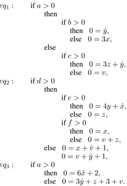
Consider for example the following DAS.
eq1: if a > 0 then if b > 0 then 0 = ˙y, else 0 = 3x, else if c > 0 then 0 = 3z + ˙y, else 0 = v, eq2: if d > 0 then if e > 0 (7) then 0 = 4y + ˙x, else 0 = z, if f > 0 then 0 = x, else 0 = v + z, else 0 = x + ˙v + 1, 0 = v + ˙y + 1, eq3: if a > 0 then 0 = 6 ˙x + 2, else 0 = 3 ˙y + z + 3 + v.
Observe that eq2 can be decomposed into two
sub-equations : eq0 2: if d > 0 then if e > 0 then 0 = 4y + ˙x, else 0 = z, else 0 = x + ˙v + 1, eq00 2 : if d > 0 then if f > 0 then 0 = x, else 0 = v + z, else 0 = v + ˙y + 1.
Therefore, system (7) can be expressed by
(eq1, eq20, eq200, eq3) Thus any conditional equation of
a DAS with embedded conditions may decompose into
smaller conditional sub-equations. In the sequel we
consider systems that are minimal, that is to say in which the conditionals equations cannot decompose anymore. As for the non-embedded DAS, we suppose that each conditional equation generates the same number of simple equations for each combination of conditions. We also suppose, without loss of generality, that every conditional equation, may generate exactly one simple equation. Given a DAS with embedded equations we will call combination
of conditions any assignment of the values true and false
to the conditions of an equation of the system. By our hypothesis any combination of condition yields only one simple equation.
For instance, in system (7), the equation 0 = ˙y in eq1is the
result of the combination {a > 0, b > 0} and 0 = v + z in eq00
2 is the result of the combination {d > 0, f ≥ 0}.
Let C1, ..., Cmbe the possible combinations of conditions. Remark that the number of combinations Ckis polynomial in the size of the system (number of simple equations and variables).
For system (7), we have the following combinations : C1=
{a > 0, b > 0}, C2 ={a > 0, b ≤ 0}, C3 ={a ≤ 0,
c > 0}, C4 ={a ≤ 0, c ≤ 0}, C5 ={d > 0, e > 0},
C6={d > 0, e ≤ 0}, C7={d > 0, f > 0}, C8={d > 0,
f ≤ 0}, C9 =d ≤ 0, C10 =a > 0 and C11 =a ≤ 0. For
i = 1, ..., m, let Ribe the set of combinations of conditions that are implied by Ci, that is the combinations that are satisfied if Ci so is. For instance, for the example above,
C10= {a > 0} is implied by C1 = {a > 0, b > 0}. For
i = 1, ..., m, let Ti be the set of combinaisons Cj which are incompatible with Ci, that is Ci and Cj cannot occur at the same time. For the example above C2 and C4 are
incompatible.
Consider the bipartite graph G = (U ∪ V, E) where U =
{u1, ..., un} corresponds to the conditional equations of the system, V = {v1, ..., vn} corresponds to the variables, and we consider an edge uivibetween two nodes ui ∈ U and
vi ∈ V if the variable viappears in a simple equation that may be generated by the conditional equation correspond-ing to ui, when a combination Ckof conditions holds. Let Ekbe the set of edges implied by combinations Ck, for
k = 1, ..., n. Thus
E = [
k=1,...,m
Ek.
For system (7), the edge sets Ek, generated by combination
C1, ..., C11, are E1 = { u1v2 }, E2 = { u1v1 }, E3 =
{ u1v3, u1v2 }, E4 = { u1v4 }, E5 = { u2v2, u2v1 },
E6 = { u2v3 }, E7 = { u3v1 }, E8 = { u3v4, u3v3 },
E9 = { u2v1, u2v4, u3v4, u3v2 }, E10 = { u4v1 } and
E11 = { u4v2, u4v3, u4v4}. And the incidence graph is
given in Figure 5. Note that nodes u2, u3correspond to the
conditional equations eq0
2, eq200. The number on each edge
corresponds to the set Ekto which belongs the edge.
Fig. 5: Graph G.
Thus the DAS is bad-constrained if and only if there exists a family F of sets Ek whose edges cover the nodes of U
and such that the subgraph induced by these edges does not contain a perfect matching. Moreover, F must satisfy the following :
a) if Ei, Ej ∈ F , then Ciand Cjare compatible, and b) if Ei∈ F and Cj ∈ Ri, then Ej∈ F .
One can easily verify, for graph G of Figure 5 that the sets
E1, E6, E7, E10constitute a feasible family that covers the
nodes u1, ..., u4 and verifies the conditions a), b) above.
However the subgraph induced by there sets does not tain a perfect matching. In consequence, the family of con-ditions C1, C6, C7, C10induces a bad-constrained system.
Given a DAS with embedded conditions we will call state of the system any set of combinations Ci covering all the equations of the system and whose edge sets Eiverify con-ditions a), b) above.
As for the DASs studied in the previous section, the prob-lem here is to find a state in which the system is bad-constrained or to show that the system is well-bad-constrained in any state. So in graph G this consists in finding a sub-graph induced by a state of the system which does not con-tain a perfect matching, or to show that for any state the corresponding graph contains such a matching.
7. Formulation
With every set of edges Eiwe associate a binary variable
xi such that xi = 1 if Ci is considered in the state of the system and xi= 0 if not. Clearly, if x represents a state of the system, then x satisfies the following inequalities
xi+ xk≤ 1, for all k ∈ Ri, for i = 1, ..., n,
xk ≤ xi, for all k ∈ Ti, for i = 1, ..., n. Moreover if M is a perfect matching of G, then x satisfies the equation
m X j=1
|Ej∩ M | xj= n.
Thus, by considering the following constraint, one can dis-card this solution.
m X j=1
|Ej∩ M | xj≤ n − 1.
Consider the following integer program ( bP ).
max y (12) m X j=1 |Ej∩ M | xj≤ n − 1, for all M ∈ M, (13) xi+ xk≤ 1, for all k ∈ Ri, (14) xk ≤ xi, for all k ∈ Ti, (15) X i=1,...,n Ek∩ δ(ui)6=∅ xk ≥ y, for all ui∈ U , (16) 0 ≤ xk≤ 1, for all Ek ∈ E, (17) 0 ≤ y, (18) xk ∈ {0, 1}, for all Ek ∈ E. (19) We claim that the SAP is equivalent to program ( bP ). In
fact, let (x, y) be a solution of ( bP ). If y ≥ 1, then by
constraints (16) each node of U has at least one incident edge in the bipartite graph induced by x. As this subgraph does not contain a perfect matching, this implies that the system is bad-constrained. If y < 1, as the program is to maximize y, there should not exist a state of the system such that the corresponding edge sets Eicover the nodes of
U and do not induce a perfect matching. This implies that
the system is well-constrained. Clearly, constraints (14)-(18) can be separated in polynomial time (by enumeration). For constraints (13), the separation problem can be solved to the maximum weight matching problem in a bipartite graph.
8. Conclusion
In this paper we have studied the SAP for conditional DASs. We have proposed integer programming formula-tions for the problem for both the embedded and nonem-bedded cases. We have shown that the linear relaxations of these models can be solved in polynomial time. Based on these formulations, we are now going to develop branch-and-cut algorithms for solving the problem in both versions with and without embedded conditions.
Acknowledgments
We would like to thank S´ebastien Furic, Djilali Talbi and Bruno Lacabanne from LMS-Imagine for stimulating dis-cussions. This work has been supported by the project ANR-06-TLOG-26-01 PARADE. The financial support is much appreciated.
REFERENCES
[1] K. E. Brenan, S. L. Campbel, L. R. Petzold, “Numer-ical solution of initial value problems in
differential-algebraic equations”, New York: North-Holland,
1989.
[2] I. Duff, “Analysis of sparse systems”, Thesis - Oxford
university, 1972.
[3] A. L. Dulmage, N. S. Mendelsohn, “Coverings of bi-partite graphs”, Canadian Journal of Mathematics, 1963, pp. 517-534.
[4] J. Edmonds, “Maximum matching and a polyhedron with 0,1-vertices”, J. Res. Nat. Bur. Standards 69B, 1965, pp. 125-130.
[5] P. Fritzson, “Principles of Obeject-Oriented Mod-eling and Simulation with Modelica 2.1”,
Wiley-Interscience, 2003.
[6] M. Grtschel, L. Lovasz, A. Schrijver, “The ellipsoid method and its consequences in combinatorial opti-mization”, Combinatorica 1, 1981, pp. 169-197. [7] D. Jian-Wan, C. Li-Ping, Z. Fan-Li, W. Yi-Zhong,
W. Guo-Biao, “An Analyzer for Declarative Equation Based Models”, Modelica 2006, 2006, pp. 349-357. [8] A. Leitold, K. M. Hangos, “Structural solvability
analysis of dynamic process models”, Computeurs
and Chemical Engineering 25, 2001, pp. 1633-1646.
[9] L. Lovasz, M. D. Plummer, “Matching Theory”,
North-Holland, 1986.
[10] K. Murota, “Systems Analysis by Graphs and Ma-troids”, Springer-Verlag, 1987.
[11] K. Murota, “Matrices and Matroids for Systems Anal-ysis”, Springer-Verlag, 2000.
[12] G. L. Nemhauser, L. A. Wolsey, “Integer and Com-binatorial Optimization”, A Wiley-Interscience
Publi-cation, 1988.
[13] H. Nilsson, “Type-Based Structural Analysis for Modular Systems of Equations”, Proceedings of
the 2nd International Workshop on Equation-Based Object-Oriented Languages and Tools, 2008, pp.
71-81.
[14] G. Reibig, U. Feldmann, “A simple and general method for detecting structural inconsistencies in large electrical networks”, Circuits and Systems I:
Fundamental Theory and Applications, 2002, pp.
237-240.
[15] J. Unger, A. Kroner, W. Marquardt, “Structural anal-ysis of differential-algebraic equation systems - the-ory and application”, Computeurs and Chemical