2017 — Development of a New Multi-Channel MRI Coil Optimized for Brain Studies in Human Neonates

(1)

UNIVERSITÉ DE MONTRÉAL

DEVELOPMENT OF A NEW MULTI-CHANNEL MRI COIL OPTIMIZED FOR BRAIN STUDIES IN HUMAN NEONATES

NIBARDO LOPEZ RIOS

DÉPARTEMENT DE GÉNIE ÉLECTRIQUE ÉCOLE POLYTECHNIQUE DE MONTRÉAL

THÈSE PRÉSENTÉE EN VUE DE L’OBTENTION DU DIPLÔME DE PHILOSOPHIAE DOCTOR

(GÉNIE ÉLECTRIQUE) NOVEMBRE 2017

(2)

UNIVERSITÉ DE MONTRÉAL

ÉCOLE POLYTECHNIQUE DE MONTRÉAL

Cette thèse intitulée :

DEVELOPMENT OF A NEW MULTI-CHANNEL MRI COIL OPTIMIZED FOR BRAIN STUDIES IN HUMAN NEONATES

présentée par : LOPEZ RIOS Nibardo

en vue de l’obtention du diplôme de : Philosophiae Doctor a été dûment acceptée par le jury d’examen constitué de :

M. LESAGE Frédéric, Ph. D., président

M. COHEN-ADAD Julien, Ph. D., membre et directeur de recherche M. DEHAES Mathieu, Ph. D., membre et codirecteur de recherche M. CALOZ Christophe, Ph. D., membre

(3)

DEDICATION

(4)

ACKNOWLEDGEMENTS

First, I would like to express my special appreciation to my supervisors Prof. Julien Cohen-Adad and Prof. Mathieu Dehaes, for their support and trust. I would like to thank them for giving me the opportunity to work on such exciting projects. I also want to express my immense gratitude for the constructive discussions, advise and direct help with experiments. I am very fortunate to be allowed work in the highly skilled research group and pleasant environment that Prof. Julien Cohen-Adad has created.

I would like to thank my thesis committee, Prof. Frédéric Lesage, Prof. Christophe Caloz and Prof. Jamie Near for accepting to participate in my defense. My sincere appreciation for using your time to read and evaluate my manuscript, and for your brilliant comments and suggestions.

I thank also Prof. Gregory Lodygensky for the valuable advice and collaboration since the very beginning of the project. I thank our collaborators Fraser Robb, Miguel Navarro, Pei H. Chan, Jorge Guzman, and Kellie Tribbey from GE Healthcare for their valuable support, technical assistance and encouragement. I appreciate also the aid received from Brian A. Hargreaves from Stanford University. I also thank Jonathan Polimeni from the MGH Martinos Center for sharing his code to compute the SNR.

I would like to acknowledge the funds received by the Canada Research Chair in Quantitative Magnetic Resonance Imaging, the Canadian Institute of Health Research (CIHR FDN-143263), the Canada Foundation for Innovation (32454), the Fonds de Recherche du Québec - Santé (28826, 32600), the Fonds de Recherche du Québec - Nature et Technologies (2015-PR-182754), the Natural Sciences and Engineering Research Council of Canada (435897-2013, 2015-04672), the Québec Bio-Imaging Network (5886) and a fellowship from the CREER (FRQNT).

I thank my lab mate Alexandru Foias for the great discussions and his valuable support in many aspects. In addition, I would like to thank Prof. Nikola Stikov and my fellow students and researchers Tanguy Duval, Benjamin De Leener, Ryan Topfer, Gabriel Mangeat, Grégoire Germain, Sara Dupont, Charley Gros, Simon Lévy, Tommy Boshkovski, Agah Karakuzu, Manh-Tung Vuong, Aldo Zaimi, Atef Badji, Christian Perone, Stephanie Alley, Ariane Saliani, Hadi Begdouri, Harris Nami, Pierre-Olivier Quirion, George Peristerakis, Jennifer Campbell, Darya Morozov, Pascale Beliveau and many others for their support and for being such a nice workgroup.

(5)

I thank also Prof. Frédéric Lesage and Philippe Pouliot for their important support with related research. Many thanks also to all my Professors for such interesting courses and workshops. I would like to thank my family and friends: especially to my wife Linnet for her love and for being always so supportive; to my parents Nibardo and Melvis, to my brothers Jose Enrique and Pedro, and my daughter Laura for their vital support, and finally to my son Mario for being a new motivation for everything. To my friends and colleagues in Cuba for their preoccupation and valuable help in difficult moments. Without all of them, this work would not have been so pleasant.

(6)

RÉSUMÉ

Plusieurs événements et conditions indésirables causent des lésions cérébrales chez les nouveau-nés qui peuvent conduire plus tard à des troubles neurodéveloppementaux. Des études d'imagerie rapides, non invasive et de haute qualité sont nécessaires pour initier un traitement neuroprotecteur précoce et minimiser les effets néfastes sur ces patients. L'imagerie par résonance magnétique (IRM) est une méthode de choix pour détecter ces lésions et évaluer le développement du cerveau in vivo. Les systèmes d'IRM comprennent des antennes spécifiques qui permettent d’interagir avec l'objet étudié au moyen de signaux radiofréquences (RF). Ces antennes jouent un rôle important sur la qualité d'image résultante et donc sur notre capacité à détecter des pathologies subtiles. Plus les antennes sont proches du tissu à imager, meilleure est la qualité d’image.

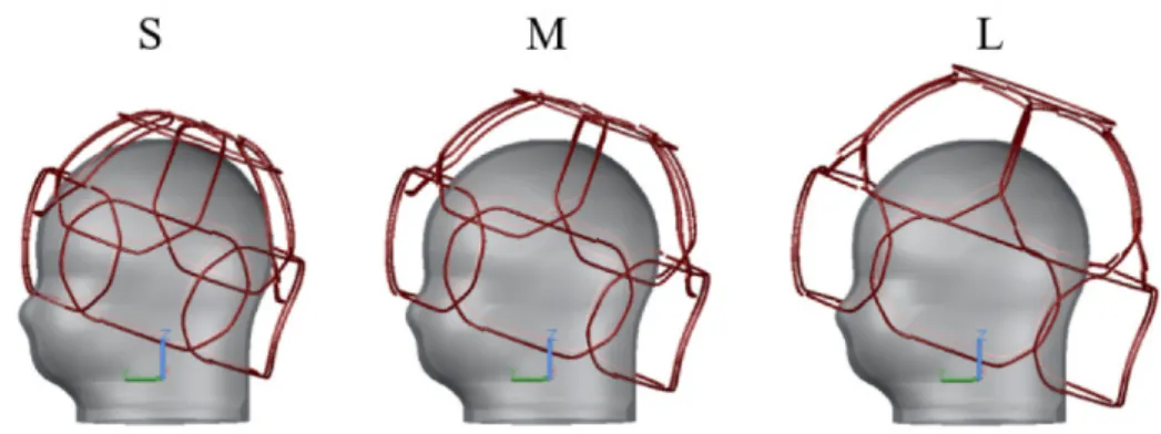
Le but de ce travail était de développer une nouvelle antenne de réception IRM qui peut s'adapter physiquement à la taille de la tête des nouveau-nés dans la gamme de prématurés de 24 semaines à des bébés de 1.5 mois.

L'antenne est constituée de treize éléments répartis de manière sphérique, fixés individuellement à un soufflet en plastique compressible, qui peuvent se déplacer de manière indépendante dans des directions radiales et axiales. Un système pneumatique les rétracte au moyen d'un vide, en maximisant l'espace à l'intérieur de l'antenne pour faciliter le placement du sujet. Le vide est ensuite libéré pour permettre l'expansion du soufflet et le mouvement des éléments vers le centre de l'antenne jusqu'à ce qu'ils s'adaptent physiquement à la forme de la tête. La simulation électromagnétique a aidé le processus de conception, révélant la faisabilité de l'idée proposée. Un découplage efficace à l’aide de préamplificateurs a garanti les niveaux requis de découplage global entre les canaux de l’antenne. La validation a été effectuée sur le banc d’essai et sur une IRM 3T en utilisant différents fantômes en forme de tête.

Les résultats démontrent une augmentation moyenne de rapport signal-à-bruit (SNR) de jusqu'à 68% dans la région de la tête et 122% dans la région du cortex, par rapport à une antenne commerciale de tête à 32 canaux. La distribution du SNR est stable pour toutes les tailles de fantômes utilisés.

En conclusion, une antenne de réception a été conçue, modélisée puis construite. Cette antenne est adaptable avec contrôle pneumatique, ce qui a permis un SNR plus élevée par rapport à une antenne de tête commerciale à 32 canaux utilisée normalement dans la pratique clinique. Les risques

(7)

associés à la pression mécanique sur la tête des nouveau-nés sont inexistants (utilisation de pression négative versus positive) et le mouvement de la tête est restreint. En plus, la méthode a des applications potentielles à d'autres groupes d'âge et parties du corps.

(8)

ABSTRACT

Several adverse events and conditions cause brain injury in neonates that can later lead to neurodevelopmental disabilities. Fast, non-invasive and high-quality image studies are required to initiate early neuroprotective treatment and minimize adverse effects on these patients. Magnetic Resonance Imaging (MRI) is a vital method to detect these injuries and assess brain development in vivo. The MRI systems include specific types of antennas, commonly known as radiofrequency (RF) coils, to interact with the object under study by means of RF signals. These coils play a strong role on the resulting image quality and hence on our ability to detect subtle pathologies. The closer the coils are to the scanned tissue, the better the image quality.

The purpose of this work was to develop a new MRI RF receiver array coil that can physically adapt to infant head sizes from 24-week premature to 1.5-month-old.

The coil is made of thirteen spherically distributed elements, individually attached to compressible plastic bellows, that can independently move in radial and axial directions. A pneumatic system retracts them by means of vacuum, maximizing the space inside the coil to facilitate the placement of the subject. The vacuum is afterward liberated to allow the expansion of the bellows and the movement of the elements toward the coil center until they physically adapt to the head shape. Electromagnetic simulation assisted the design process, revealing the feasibility of the proposed idea. A strong preamplifier decoupling guaranteed the required levels of overall decoupling among the coil elements. The validation was performed on the bench and on a 3T scanner using different head-shaped phantoms.

The results show up to up to 68% in the head region and 122% in the cortex region, compared to a 32-channel commercial head coil. A stable SNR distribution through the complete size range was also obtained for all the used phantoms.

In conclusion, an MRI receiver coil was designed, modeled, and built. The coil is adaptable with pneumatic control, which allowed a higher SNR compared to a commercial 32-channel head coil used normally in clinical practice. The risks associated with mechanical pressure on the head of newborns are non-existent (use of negative versus positive pressure) and the head motion is restricted. In addition, the method has potential applications to other age groups and body parts.

(9)

LIST OF TABLES

Table 4.1 Part values used to tune and match the loops to 150 Ohm... 78

Table 5.1 Loop impedance and tuning/matching capacitors. ... 88

Table 5.2 Impedance of the tuned/matched loops for all sample dimensions. ... 88

Table 5.3 Tuning and matching capacitances for geometrical decoupling. ... 90

Table 5.4 Tuning and matching capacitances of the final configuration. ... 90

Table 5.5 Actual loop impedances and tuning/matching capacitors. ... 102

Table 5.6 Impedance of the tuned/matched loops for all phantoms. ... 103

Table 5.7 Quality factors of the independent loops. ... 103

Table 5.8 Tuning frequency shift due to the loading. ... 103

Table 5.9 Impedance measurements after the assembly of the array. ... 105

Table 5.10 Frequency shift with respect to the tuning condition (M size). ... 105

Table 5.11 QL test in the array. ... 107

(16)

LIST OF FIGURES

Figure 2.1 Simplified block diagram of an MRI system. ... 5 Figure 2.2 Nuclei spinning around their own axis and oriented in random directions when no

external magnetic field (B0 = 0) is applied. Each nucleus behaves as a very small magnet as

shown on the top left corner. ... 6 Figure 2.3 The spin system of Figure 2.2 placed in a magnetic field. On the left, all magnetic

moments are precessing around opposite directions along the z-axis: parallel (blue z-axis) and antiparallel (red z-axis). On the top right, the spin system is represented as two precessing cones formed by the magnetic moment vectors. The precession motion is illustrated by the movement of a spinning top on the bottom right. ... 7 Figure 2.4 M movement caused by B1 in the rotating frame (left), and in the conventional or

laboratory frame (right). ... 10 Figure 2.5 Partial trajectory of M after the RF pulse is switched off. The projection on the transverse plane induces a current in a receiver coil (in red) placed perpendicularly to the x-axis. ... 10 Figure 2.6 Curves that describe the longitudinal relaxation (top) and the transversal relaxation (bottom) after a 90o_{pulse. In these conditions 𝑀𝑀𝑀𝑀′0+= 0 and 𝑀𝑀𝑀𝑀′𝑡𝑡 in Equation 1.16 has only}

the first term on the right. ... 11 Figure 2.7 FID of a spin system having only one spectral component in an inhomogeneous

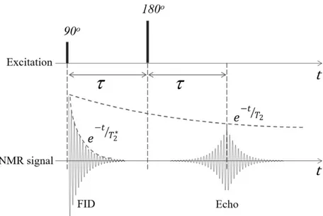
magnetic field. ... 12 Figure 2.8 Evolution of the transverse magnetization due to a 90-τ-180 RF pulse sequence. ... 13 Figure 2.9 NMR signals due to a 90-τ-180 RF pulse sequence. Notice the 𝑇𝑇2 ∗ dependence of the FID and the T2 dependence of the echo. ... 14

Figure 2.10 Spatial encoding. a) two possible selected slices on a human head having the Larmor frequency at the eyes and a higher frequency at the head. b) phase encoding reached by previously applying a time invariant frequency gradient Gy(t). All signals start with the same

phase but at the end of the pulse they have a different phase. c) 3 x 3 matrix representing one selected slice from a) (the one at 𝜔𝜔0) where the phase-encoded signals from b) are

(17)

subsequently frequency-encoded by means of another time invariant frequency gradient (Gx(t)). Notice that each member of the matrix has a unique combination of phase and

frequency. ... 16

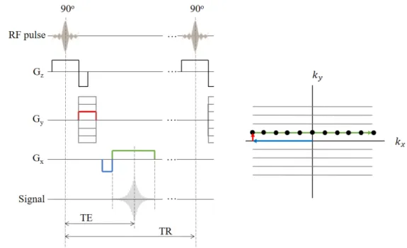
Figure 2.11 Diagram of the Gradient Recalled Echo (GRE) pulse sequence and the trajectory of the magnetization in k-space. ... 18

Figure 2.12 Equivalent circuit of a series tuned coil. ... 20

Figure 2.13 Series (a) and parallel (b) resonant circuits commonly used in RF coils. RL is the source impedance required for noise match, usually 50 Ohm. ... 21

Figure 2.14 Surface coils and typical sensitivity. a) Relative sensitivity of two surface coils with different diameters (φ). b) A few common topologies used to build surface coils. ... 23

Figure 2.15 Critical overlapping for geometric decoupling between two squared (a) and circular (b) loops. The currents induced in coil 2 due to a current circulating in coil 1 are added in b). Notice that equal numbers of magnetic flux lines cross coil 2 in opposite directions, inducing equal currents that mutually cancel. ... 25

Figure 2.16 Simplified circuit that illustrates the principle of preamplifier decoupling, adapted from Roemer’s work [8]. ... 26

Figure 4.1 Array configuration loaded with a medium size spherical sample. Element 1 has a circular shape and is located at the top of the array. Elements 2 to 7, having a trapezoidal shape, are placed in the top row and elements 8 to 13, with a rectangular shape, make up the bottom row. Notice that the corners of elements 2 to 13 are chamfered. A decoupled double probe is shown on top of element 1... 46

Figure 4.2 Initial coil model. a) Soccer-ball pattern drawn on a fixed-size helmet made for a 32-channer array where only one loop is placed. The other loops will be concentrically placed with the pentagons and hexagons. b) Isometric view of the initial array configuration made with circular loops. c) Array adjusted to the maximum and minimum sizes. ... 51

Figure 4.3 Electrical design selected for all coil elements. ... 52

Figure 4.4 Selected preamplifier with electrical schematic and parameters. ... 54

(18)

Figure 4.6 Loop test model, and tuning and matching curves. a) The ports and loads used for tuning/matching and a double probe on the M size load. b) The S11 parameter measured at the

loop output. c) S21 measured between the double probes. ... 55

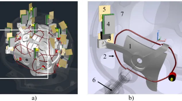
Figure 4.7 Some transformations performed on the loops to find the geometrical decoupling. .... 57 Figure 4.8 Simulated array before and after geometrical decoupling. ... 58 Figure 4.9 Model of the preamplifier. a) Schematic of the input transformer of a preamplifier. b) Ports and loads used in FEKO to model the preamp, shown here in loop-1. ... 59 Figure 4.10 Decoupling evaluation by magnetic field simulations. ... 61 Figure 4.11 AutoCAD model of the loop array adjusted to the extreme and medium loads. ... 62 Figure 4.12 Partial AutoCAD 3D model of the coil. a) Adjustable helmet in the S dimension. Some parts are turned off to simplify the view. The section in the white square was magnified in b) and other parts were removed to show only the element 12. The coordinate system was placed in the geometrical center of the array, with the z axis in parallel with B0 field. The support (1)

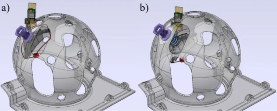
holds the wire loop (2) and the matching/detuning board (3) where the preamplifier (4) and the output/filter board (5) are plugged. Notice the alignment of the preamplifier with the z axis. The element will move along an axis starting from the coil center (6). A fixed-size spherical frame (7) surrounds the array of elements. ... 63 Figure 4.13 3D drawings of all coil elements. ... 63 Figure 4.14 X-Ray view of the spherical frame. The element 5 is shown in the retracted (a) and the extended (b) positions. ... 64 Figure 4.15 Different types of bellows. The parts shown on the right were used for this study as they are commercially available. ... 64 Figure 4.16 Pneumatic system used to move the array. The ensemble of the bellows (1) and the tubing (2) is connected to a vacuum source (3), which in this case was a hand pump. A check valve (4) retains the vacuum inside the system until a manually operated air valve (5) is open. ... 65

(19)

Figure 4.17 Illustration of the tilting movement described by the loops after they touch the surface of the sample. The loop will move parallel to the displacement axis (dashed lines) and will rotate (red arrow) to adapt the head shape. ... 66 Figure 4.18 External view of the 3D model of the coil. a) Housing with maximum dimensions. b) Detail of the bed holding a phantom (S). Some parts are transparent and other are removed for clarity. The height of the bed can be adjusted (white arrows) according to the size of the patient. ... 67 Figure 4.19 Steps followed to select the shape of the phantom. The final shape was similar to the normocephalic head (1), which is the medical term used for babies with normal head dimensions and proportions. ... 67 Figure 4.20 Printed plastic parts. a) Element 1 after printing with the required supports. b) Element 3 on top of one of the three molds printed to shape the wires (loops 2 to 7 in this case). c) Hollow screw and nut used to fix the bellows to the spherical frame. d) Spherical frame with three elements already mounted. e, f) Strain reliefs used to protect the cable and reinforce the attachment to the coil housing and the P connector. ... 68 Figure 4.21 Picture of the coil housing with the spherical frame, which is also a part of the external assembly. ... 68 Figure 4.22 Set of phantoms used to test the coil. ... 69 Figure 4.23 Part of element 3 containing the loop soldered to the matching/detuning board and both attached to the support. The three fixing joints are shown. ... 69 Figure 4.24 Coil cable with all cable traps and output boards connected. Some preamplifiers are plugged to the output boards. The P connector is open showing the coil ID card. ... 70 Figure 4.25 Assembly of the coil elements in the spherical frame. The preamplifier of the element 1 is connected on the right picture. The input tubes of the bellows were bent to use the space more efficiently. ... 71 Figure 4.26 Constructed test box. The schematic of channels 1 and 2 with the DC voltage

connectors and the PCB of channels 1,2, 31 and 32 are shown. A picture is shown on the right where the P connector is seen at the bottom. ... 72

(20)

Figure 4.27 Constructed test probes. 1, 2 and 5 are decoupled double probes made of critically overlapped single magnetic field probes, like 6. 1 and 2 have the same structure but the size of the part that contains the loops is different. 3 is a parallel double probe. 4 and 7 are

solenoidal probes also called sniffing probes. ... 73

Figure 4.28 Calibration and test devices. a) Calibration kit for improving impedance measurements. b) Dummy preamplifier. c) and d) Impedance L-type transformer networks made with variable components. ... 73

Figure 4.29 Preamplifier specifications and electric design of 4-channel array. ... 74

Figure 4.30 Picture of the 4-channel array. ... 75

Figure 4.31 WMM miniature 6-pin preamplifier and measured parameters. ... 76

Figure 4.32 Coil element architecture used for 150-Ohm preamplifier. ... 76

Figure 4.33 Setup to evaluate preamplifier decoupling effect according to distance between loops. ... 77

Figure 4.34 PCB for 6-pin miniature preamplifier. ... 78

Figure 4.35 Setup to evaluate the effect of the preamplifier decoupling between complete array elements. ... 79

Figure 4.36 Impedance measurement setup to find the loop inductance (a) and one result (b). .... 80

Figure 4.37 Loop output impedance measurement setup (a) and one result after the adjustment(b). ... 80

Figure 4.38 Setup used to perform decoupling tests (a) and a typical Q measurement results (b).81 Figure 4.39 Typical results of the active detuning (a) and preamplifier decoupling (b). ... 82

Figure 4.40 Setup used to measure the interaction (S21) between loops (a) and a typical result (b) showing very good matching of both elements (top) and a good decoupling (bottom). The span was 40 MHz. ... 84

Figure 4.41 Setup used to measure the frequency response of the array elements (a) and typical dog-ear shape obtained from an isolated channel. ... 85

(21)

Figure 5.2 Simulated active detuning. ... 88

Figure 5.3 S21 achieved between loops by geometrical decoupling. The adjusted loops are shown in each graph along with the S11 curve for each loop. ... 89

Figure 5.4 S-parameters matrices of the simulated geometrically decoupled array. ... 90

Figure 5.5 S-parameters matrices of the final simulated array. ... 91

Figure 5.6 Preamplifier decoupling evaluation by simulations. ... 91

Figure 5.7 S-parameter matrices after the inclusion of the preamplifiers. ... 92

Figure 5.8 Preamplifier decoupling test on two loops. ... 92

Figure 5.9 Sample of the preamplifier decoupling evaluation in the complete array. ... 93

Figure 5.10 Magnetic field intensity maps comparison. ... 94

Figure 5.11 Axial B1- maps at a quarter of the sphere diameter above the center plane. ... 94

Figure 5.12 Axial B1- maps at the center plane. ... 95

Figure 5.13 Axial B1- maps at one quarter of the sphere diameter below the center plane. ... 95

Figure 5.14 Photographs of the constructed coil in the extreme dimensions. Some important parts such as the manually operated air valve (1), the bellows (2), the hand pump (3) and the check valve (4) are shown in the working assembly. 3D drawings of the loops distributions are presented in the corresponding lower left corners of the coil pictures. c) Closed (S) coil detail on the element 10 showing the bellows (5), the preamplifier (6), the support (7), the wire loop (8) and the matching board (9). ... 96

Figure 5.15 Preamplifier decoupling evaluation of the 4-channel array prototype. ... 97

Figure 5.16 Bench test results of the Siemens 4-channel array with 50 Ohm noise match. ... 98

Figure 5.17 Parameters measured of the coil element made with the150-Ohm WanTcom preamplifier. The frequency span was 40 MHz. ... 98

Figure 5.18 Results of preamplifier decoupling effectiveness test. ... 99

Figure 5.19 Preamplifier decoupling related to the distance between loop centers. A WanTcom WMM series miniature 6-pin preamplifier was used. The frequency span was 40 MHz. ... 100

(22)

Figure 5.20 Preamplifier decoupling evaluation regarding the distance between loop centers with the MPB-127R73-90. The frequency span was 40 MHz. ... 101 Figure 5.21 Sample of Q measurement (loop 7). a) QU. b) Overlapped QL measurements with the

three phantoms. The frequency span was 10 MHz. ... 104 Figure 5.22 Preamplifier decoupling assessment of all channels. An average of -25 dB was

achieved. 1) Curves measured with the loop terminals open. 2) Loops terminals loaded with a 180Ohm resistor. 3) Preamplifiers connected to the loops. ... 104 Figure 5.23 Impedance measurements in the assembled array. The curves of the 13 elements are overlapped. The frequency span is 40 MHz. ... 106 Figure 5.24 S21 values between pairs of loops (1 to 7) presented as color matrices. ... 107

Figure 5.25 Overlapped sensitivity profiles of all coil elements for each load size. ... 108 Figure 5.26 Noise correlation matrix and SNR map of the 4-channel array. ... 108 Figure 5.27 Images acquired on a non-homogeneous sample. ... 109 Figure 5.28 Axial and sagittal SNR maps computed for the 10cm spherical phantom. Small

dot-shaped oscillation artifacts are pointed with white arrows. ... 109 Figure 5.29 Noise correlation matrices computed for all phantoms and both coils and noise

acquisition from each channel of the proposed coil with the M phantom. ... 110 Figure 5.30 Axial and sagittal slices acquired with the proposed coil loaded with the M phantom.

... 111 Figure 5.31 Previous axial and sagittal acquisitions repeated after some improvements. ... 111 Figure 5.32 Axial images of the three constructed phantoms. The intensity scaling is the same

everywhere. ... 112 Figure 5.33 Sagittal images of all phantoms. The intensity scaling is the same everywhere. ... 112 Figure 5.34 Noise correlation matrices computed for both coils and off-diagonal averages. ... 113 Figure 5.35 Axial SNR maps of all the three constructed phantoms. ... 114 Figure 5.36 Sagittal SNR maps of all phantoms. The edges of the masks used to select the region of interest are shown in each image. ... 114

(23)

List of symbols and abbreviations DTI Diffusion tensor imaging ESR Equivalent Series Resistance FEM Finite Element Method FID Free induction decay FOV Field-of-view

GE General Electric

GRE Gradient Recalled Echo iSNR Intrinsic signal-to-noise ratio MoM Method of Moments

MPRAGE Magnetization Prepared Rapid Gradient Echo MR Magnetic resonance

MRI Magnetic resonance imaging MRS Magnetic resonance spectroscopy

NF Noise figure

NMR Nuclear magnetic resonance PCB Printed circuit board

PI Parallel imaging

Q Quality factor

QU Unloaded quality factor

QL Loaded quality factor

RF Radio frequency

RL Return loss

(24)

rSoS Root-sum-of-squares

Rx Receiver

SENSE SENSitivity Encoding

SMASH SiMultaneous Acquisition of Spatial Harmonics SNR Signal-to-noise ratio T1 Longitudinal relaxation T2 Transverse relaxation TE Echo time TR Repetition time Tx Transmitter Tx/Rx Transmitter/Receiver uiSNR Ultimate intrinsic SNR VLBW Very low birth weight

(25)

LIST OF APPENDICES

Appendix A – Matlab codes ... 137 Appendix B – Patent application filing recipt ... 139

(26)

CHAPTER 1 INTRODUCTION

1.1 Problem

Neonatal brain injury and abnormality due to adverse events or conditions, such as intracranial hemorrhage, stroke or vascular anomalies, are frequent in very low birth weight (VLBW) preterm infants and newborns with birth asphyxia or congenital heart disease [1], [2], [3], [4]. The injuries resulting from these events, can later lead to significant neurodevelopmental disabilities. Fast and high-quality image studies are required to initiate early neuroprotective treatment and minimize the adverse effects on the newborns. Since the clinical manifestations of the neurological diseases are very subtle in the newborn infant, mainly in the premature [4], there is a great need for high-resolution imaging of the neonatal brain. Magnetic Resonance Imaging (MRI) is currently one of the methods of choice to detect neonatal brain injury and assess brain development in vivo [5]. Advanced MRI techniques, such as magnetic resonance spectroscopy (MRS) and diffusion tensor imaging (DTI), have contributed to enrich the field of the neonatal brain studies, triggering an important amount of research and applications [5]. MRS is used to measure local brain compounds that are valuable in assessing metabolic changes associated with brain development and injury. DTI is used to characterize the three-dimensional spatial distribution of water diffusion in each voxel of the MRI scan, which provides a sensitive measure of regional brain microstructural development.

On the other hand, MRI systems include specific types of antennas, commonly known as radio frequency (RF) coils, to interact with the object under study by means of RF signals. High-energy excitation pulses are sent with a transmitter coil to the object, which afterward emits a very weak response signal that is captured by a receiver coil. These coils play a strong role on the resulting image quality and hence on our ability to detect subtle pathologies. Their design parameters are closely related to the geometry and composition of the object.

Regardless of the importance of imaging studies in infants, only a limited number of fixed-size receiver coils for the neonatal brain is commercially available, among which a few arrays can be distinguished [6], [7]. It was demonstrated that higher image Signal-to-Noise Ratio (SNR) is obtained by means of receive array coils closely positioned on the subject [8]. On the other hand, it is known that the dimensions and shape of the head in the pediatric population are highly variable,

(27)

mainly during the first weeks of age when the brain is undergoing maturational processes. Accordingly, the performance of a fixed-size coil is optimal for the largest head that fits into it while it shows poorer image parameters as the head dimensions reduce. This is even worse in the clinical practice, where standard adult head or knee coils are used. In these cases, the difference in dimensions is even bigger, as the inner diameter of an adult coil is around 24 cm. Some commercial flexible coils and pediatric birdcages are also used, but they do not have the best potential for neonatal brain studies due to their cylindrical configuration, among other disadvantages. To improve SNR with these alternatives, the typical solutions involve longer scan times, which is more likely to produce images with increased motion artifacts and may affect the physiological conditions of these most vulnerable patients.

A few optimized but not commercially available pediatric head coils were proposed. One approach is based in a set of age-matched arrays that resulted in optimal images, but it also has practical inconveniences related to cost and workflow [9], [10]. These results were the main motivation for subsequent efforts, including the present work. A different approach is based on adjustable coils based in arrays divided in two or four sections that are moved by means of actuators [11], [12], [13], [14]. The ideas presented in these works might be used to build a neonatal coil, but no evidence of a constructed adjustable coil for infants was found during this project. In addition, these ideas present potential risks for the fragile head of the neonates. More details are provided in 3.5.

1.2 Goal

The purpose of this work is to develop and evaluate a novel size-adaptable receive RF array coil which can be used to scan a variety of infant head sizes, including preterm and term babies, to increase image SNR compared to fixed-size coils.

1.2.1 General approach

The project was focused on the design, construction and evaluation of a first-of-its-kind MRI neonatal receiver array coil. The coil was specifically built for a 3T scanner (Signa MR750, GE Healthcare, Wauwatosa, WI, USA) but the same design can be applied to other MRI models or field strengths. The number of channels, dimensions and shape were optimized to obtain a high SNR in the intended population. Improved SNR compared to commercial coils, high levels of

(28)

comfort for the newborn, adjustability to the head size, simplicity of utilization of life support systems, such as endotracheal tubes and incubators, were the optimizing criteria. Improvements were also anticipated in Parallel Imaging (PI) applications.

The structure of the loops and the general decoupling among them in different conditions were evaluated by electromagnetic field simulations during the design process. 3D design and printing tools were used to model and build the coil. Phantoms of different sizes were also constructed to simulate the presence of the patients in the coil through the test stages. The array was initially adjusted and assessed in the workbench. Then, it was evaluated in the scanner by following standard methods. The results were compared to a fixed-size commercial coil.

(29)

CHAPTER 2 MRI OVERVIEW

Magnetic Resonance Imaging (MRI) is a diagnosis method that combines the use of magnetic fields of different nature with the magnetic properties of certain atomic nuclei, such as hydrogen (1_{H), to}

create very detailed images of the biological tissue. It is based on Nuclear Magnetic Resonance (NMR), a phenomenon that was discovered simultaneously and independently by Felix Bloch and Edward Mills Purcell, who received the Nobel Prize in Physics in 1952. The first 2D images were produced by Paul Lauterbur and Sir Peter Mansfield in the 1970s, who were also awarded the Nobel Prize in Physiology or Medicine in 2003 for their development of MRI. Raymond Damadian developed the first MR scanner and obtained the first human body images in 1977. MRI uses radio frequency (RF) signals that are in the commercial spectrum and does not need ionizing radiation, which makes it a safer imaging method compared to other modalities, such as X-ray, computed tomography (CT) and molecular imaging (use of radiotracers). Other important advantages of this method are the amount of information contained in the images and the possibility of adjusting the MRI protocol to boost or reduce the effects of the intrinsic parameters of the object under study, which generates images with different contrast. Cellular structure, flow and diffusion can be studied with this versatile method.

The NMR experiment can be explained in a simple way. The selected nuclei align with a strong magnetic field created by a magnet. They are rotated by using a RF pulse, and afterward they return to the equilibrium alignment oscillating in the magnetic field and emitting a RF signal at the same time.

2.1 System architecture

An MRI machine is made of several blocks among which three main components can be distinguished: the magnet, the magnetic field gradient system and the RF system. A simplified block diagram is presented in Figure 2.1. The magnet is placed in a completely shielded room (Faraday cage) to isolate the RF signals from the electromagnetic environment. The magnet generates a strong and uniform static magnetic field, known as B0, which polarizes the nuclear spins. Clinical scanners typically have B0 from 1.5 to 3 Tesla (T). The homogeneity of B0 is corrected with a lower magnetic field created by a set of active shim coils, in addition to a set of static metallic plates carefully positioned during scanner installation. The magnetic field gradient system produces controlled spatial and time dependent magnetic fields that are superposed to B0

(30)

with the purpose of signal localization. The typical range for imaging goes from 0 to 10 mT/m with switching times of 1 ms between these values. The RF system consists of a transmitter coil and a receiver coil, or other combinations. The transmitter coil is used to excite the target spin system and must generate a rotating and uniform RF magnetic field B1. The receiver coil is designed and built to have sufficient sensitivity to capture the very low signal emitted by the spins due to the excitation. Excitation pulses can have a peak power of more than 30 kW while the NMR signal is in the range of the microvolts. The MRI systems are normally equipped with a set of different receiver coils with specific designs according with the body parts. Array coils made of simple wire loops are currently the most common coil configurations for reception and, with the progressive increase of B0 fields, they are also used for transmission.

Figure 2.1 Simplified block diagram of an MRI system.

Most electronic blocks, such as power amplifiers, synthesizers, receivers and computers are installed in the technical room. The scanner is controlled by the operator from the control room.

2.2 MRI principles

2.2.1 Magnetization

Nuclei with odd number of protons or neutrons have an angular momentum 𝑱𝑱, also called spin. The atom of hydrogen, for instance, has only one proton. It is the most used element to create MRI images mainly because of its abundance in the biological tissue. Spin is usually represented by a physical rotation about its axis, as shown in Figure 2.2. The ensemble of all spins of the same type

(31)

in an object, as hydrogen, is called a spin system. It is known that a magnetic field is created around the nucleus that has finite dimensions, electrical charge and rotates around its own axis. This magnetism resembles the field created by a very small magnet. It is called magnetic moment and is represented by a vector quantity 𝝁𝝁. The magnetic moment is related to the angular moment by [15]:

𝝁𝝁 = 𝛾𝛾𝑱𝑱 = 2𝜋𝜋𝛾𝛾𝑱𝑱 (2.1)

where 𝛾𝛾 is the gyromagnetic ratio, which is a physical constant that is different for each nucleus. For 1_{H, 𝛾𝛾 = 2.65 x 108 rad/s/T and 𝛾𝛾 = 42.58 MHz/T. The direction of 𝝁𝝁 is random due to the}

thermal motion if no external magnetic field exists. In consequence, the net magnetization of a macroscopic object is zero.

Figure 2.2 Nuclei spinning around their own axis and oriented in random directions when no external magnetic field (B0 = 0) is applied. Each nucleus behaves as a very small magnet as

shown on the top left corner.

When a spin system in placed in a magnetic field, a nuclear macroscopic magnetism, which is the physical basis of the MRI, appears. The external magnetic field is conventionally called B0 and it is parallel to the z-axis of the MRI frames, so that:

𝑩𝑩0 = 𝐵𝐵0𝒌𝒌 (2.2)

A single magnetic moment vector of the spin system partially aligns with the external magnetic field 𝑩𝑩0 taking one of two possible orientations, parallel (↑) and antiparallel (↓), as shown in Figure

(32)

magnetization M pointing in the direction of B0. The transverse component of M is zero because the nuclei precess with random phase. Each magnetic moment also shows a motion around the z-axis called nuclear precession. This movement is analogous to the movement of a spinning top and it is described by the following equation [15]:

�𝜇𝜇𝑥𝑥𝑥𝑥(𝑡𝑡) = 𝜇𝜇𝑥𝑥𝑥𝑥(0)𝑒𝑒−𝑖𝑖𝑖𝑖𝐵𝐵0𝑡𝑡

𝜇𝜇𝑧𝑧(𝑡𝑡) = 𝜇𝜇𝑧𝑧(0) (2.3)

Figure 2.3 The spin system of Figure 2.2 placed in a magnetic field. On the left, all magnetic moments are precessing around opposite directions along the z-axis: parallel (blue z-axis) and antiparallel (red z-axis). On the top right, the spin system is represented as two precessing cones

formed by the magnetic moment vectors. The precession motion is illustrated by the movement of a spinning top on the bottom right.

The angular frequency of the nuclear precession, derived from this expression, is known as the Larmor frequency:

𝜔𝜔0 = 𝛾𝛾𝐵𝐵0 (2.4)

According to this expression the resonance frequency of a spin system is determined by the magnetic field magnitude and its gyromagnetic ratio.

The macroscopic magnetization vector M is used to characterize the spin system as a sum of all magnetic moments:

𝑴𝑴 = � 𝝁𝝁𝑛𝑛 𝑁𝑁𝑠𝑠

𝑛𝑛=1

(33)

where 𝑁𝑁𝑠𝑠 is the number of spins in the system. As stated before, 𝑴𝑴 = 0 when the system is not in

a 𝑩𝑩0 field. If the system is placed in an external magnetic field, 𝑴𝑴 will change as all spins will be

oriented in two directions. These two spin groups interact with different energy levels with the 𝑩𝑩0

field. The group with parallel alignment is in a low-energy state and the antiparallel is in a high-energy state, being the high-energy difference [15]:

∆𝐸𝐸 = 𝐸𝐸↓− 𝐸𝐸↑ = 𝛾𝛾ℎ𝐵𝐵0 = 𝛾𝛾ℎ𝐵𝐵0/2𝜋𝜋 (2.6)

where h is the Plank’s constant (6.6 x10-34_{J-s) and ℎ is equal to h/2π.}

The population difference between both groups of spins is related to this energy difference: 𝑁𝑁↑− 𝑁𝑁↓ ≈ 𝑁𝑁𝑠𝑠𝛾𝛾ℎ𝐵𝐵_{2𝑘𝑘𝑇𝑇}0

𝑠𝑠 (2.7)

where k = 1.38 x 10-23_{is the Boltzmann’s constant and T}_s_{is the absolute temperature of the spin}

system. From this expression, one can notice that only a few spins in excess are in the low-energy state, which is more stable. For example, only about nine in one million of protons will contribute to the NMR signal at 3T. This small group defines the magnitude of the net magnetization:

𝑀𝑀𝑧𝑧0 = |𝑴𝑴| =𝛾𝛾 2_ℎ2_𝐵𝐵

0𝑁𝑁𝑠𝑠

4𝑘𝑘𝑇𝑇𝑠𝑠 (2.8)

it normally points along the z-axis and is proportional to the external magnetic field and the number of spins. This is the reason why images obtained with high field scanners are preferred, as a higher number of spins in excess provides more SNR.

2.2.2 Excitation

When an external oscillating magnetic field B1(t) is applied on the spin system and it rotates in the same way as the precessing spins, the resonance condition is established. It is expressed by:

𝜔𝜔𝑟𝑟𝑟𝑟= 𝜔𝜔0 (2.9)

In this condition, the energy transmitted by a radio wave of frequency 𝜔𝜔𝑟𝑟𝑟𝑟 induces transitions of

spins between energy levels. This energy is transmitted in the MRI experiment by means of radio frequency pulses that last for microseconds to milliseconds. The magnitude, in the range of the tens of mT, is very low compared to the static magnetic field.

(34)

𝑩𝑩1(𝑡𝑡) = 2𝐵𝐵1𝑒𝑒(𝑡𝑡) cos�𝜔𝜔𝑟𝑟𝑟𝑟𝑡𝑡 + 𝜑𝜑�𝒊𝒊 (2.10)

where 𝐵𝐵1𝑒𝑒(𝑡𝑡) is the envelope of the pulse, that can have different shapes such as rectangular or sinc

(cardinal sine function), 𝜔𝜔𝑟𝑟𝑟𝑟 is the carrier frequency and 𝜑𝜑 is the initial phase. This is an x-oriented

linearly polarized field that can be decomposed into two circularly polarized fields rotating in opposite directions:

𝑩𝑩1(𝑡𝑡) = 𝐵𝐵1𝑒𝑒(𝑡𝑡)�cos�𝜔𝜔𝑟𝑟𝑟𝑟𝑡𝑡 + 𝜑𝜑�𝒊𝒊 − sin�𝜔𝜔𝑟𝑟𝑟𝑟𝑡𝑡 + 𝜑𝜑�𝒋𝒋�

+ 𝐵𝐵1𝑒𝑒(𝑡𝑡)�cos�𝜔𝜔𝑟𝑟𝑟𝑟𝑡𝑡 + 𝜑𝜑�𝒊𝒊 + sin�𝜔𝜔𝑟𝑟𝑟𝑟𝑡𝑡 + 𝜑𝜑�𝒋𝒋� (2.11)

The first term rotates clockwise and the second counterclockwise on the xy-plane, which is perpendicular to B0. For the purpose of excitation, the first term, also known as 𝐵𝐵₁+, is the useful one as it rotates in the same direction as the spins. Then, the excitation field can be expressed as:

𝐵𝐵1(𝑡𝑡) = 𝐵𝐵1,𝑥𝑥(𝑡𝑡) + 𝑖𝑖𝐵𝐵1,𝑥𝑥(𝑡𝑡) = 𝐵𝐵1𝑒𝑒(𝑡𝑡)𝑒𝑒−𝑖𝑖�𝜔𝜔𝑟𝑟𝑟𝑟𝑡𝑡+𝜑𝜑� (2.12)

The second term is called 𝐵𝐵1− and it is a field that rotates in the opposite direction of the nuclear

precession. According to the principle of reciprocity [16] the magnitude of the current induced in the receiver coil by M is proportional to the magnitude of this field. In other words, the effectiveness of the receiver coil is proportional to its efficiency as a transmitter coil.

A rotating frame of reference with its z-axis aligned with B0 and its transverse plane rotating at 𝜔𝜔₀ (and 𝜔𝜔𝑟𝑟𝑟𝑟 at resonance), is introduced to facilitate the description of the B1, or RF pulse. It is

distinguished from the conventionally used stationary frame by using x’, y’ and z’ to denote the axis. After the introduction of the necessary transformations between both frames, the use of the Bloch equation [15] shows that M performs a precession around the direction of the axis in the rotating frame where the exciting field 𝑩𝑩1(𝑡𝑡) was applied (if 𝜑𝜑 = 0, this axis will be the x’-axis).

For a rectangular RF pulse the situation in the rotating frame is similar to having B0 for a short time in the conventional frame. In this case M in the rotating frame is described by:

�

𝑀𝑀𝑥𝑥′(𝑡𝑡) = 0

𝑀𝑀𝑥𝑥′(𝑡𝑡) = 𝑀𝑀𝑧𝑧0sin(𝜔𝜔1𝑡𝑡)

𝑀𝑀𝑧𝑧′(𝑡𝑡) = 𝑀𝑀𝑧𝑧0cos(𝜔𝜔1𝑡𝑡)

0 ≤ 𝑡𝑡 ≤ 𝜏𝜏𝑝𝑝 (2.13)

where 𝜔𝜔1 = 𝛾𝛾𝐵𝐵1 . This means that M precesses around the x’-axis with angular velocity:

𝝎𝝎1 = −𝛾𝛾𝑩𝑩1 (2.14)

which is very similar to the Larmor relationship as the precession frequency depends on the applied RF field. This motion is called forced precession and it is represented in Figure 2.4.

(35)

Figure 2.4 M movement caused by B1 in the rotating frame (left), and in the conventional or laboratory frame (right).

The separation from the z’-axis, which is called tipping, creates a component in the transverse plane Mx’y’ that can be externally detected. The magnetization will tip as long as the B1 field is applied. When B1 is switched off M will stop tipping. The angle at this point, known as flip angle, depends on the magnitude of B1 and the pulse length 𝜏𝜏_𝑝𝑝. For a rectangular pulse, it is:

𝛼𝛼 = 𝜔𝜔1𝜏𝜏𝑝𝑝 = 𝛾𝛾𝐵𝐵1𝜏𝜏𝑝𝑝 (2.15)

To choose the excitation bandwidth the length of the pulse is selected first. Then, the RF power is adjusted to select the flip angle. According to (2.14), the tipping is faster if the RF power is higher. When M is tipped to the transverse plane by means of a (𝛼𝛼 =) 90o_{RF pulse, it will return to its}

alignment with the z-axis, rotating around this axis after the pulse is switched off. Its projection in the xy-plane, represented by Mxy, will obviously rotate as well, as represented in Figure 2.5. If a receiver coil is conveniently placed in that plane, the varying magnetic flux created by Mxy will induce a RF current on it, in agreement with Faraday’s law. This current is the NMR signal.

Figure 2.5 Partial trajectory of M after the RF pulse is switched off. The projection on the transverse plane induces a current in a receiver coil (in red) placed perpendicularly to the x-axis.

(36)

The return of the spin system to the previous equilibrium state, after the RF pulse is turned off, occurs in a certain amount of time where M exhibits a motion called free precession. The longitudinal magnetization Mz is totally recovered and the transversal magnetization Mxy is completely attenuated during this time. These processes are called longitudinal relaxation and transverse relaxation respectively. They are described by the following expressions, that can be obtained by solving the Bloch equations for the rotating frame [15]:

�𝑀𝑀𝑧𝑧′(𝑡𝑡) = 𝑀𝑀𝑧𝑧0�1 − 𝑒𝑒−𝑡𝑡 𝑇𝑇⁄ 1� + 𝑀𝑀𝑧𝑧′(0+)𝑒𝑒−𝑡𝑡 𝑇𝑇⁄ 1

𝑀𝑀𝑥𝑥′𝑥𝑥′(𝑡𝑡) = 𝑀𝑀𝑥𝑥′𝑥𝑥′(0+)𝑒𝑒−𝑡𝑡 𝑇𝑇⁄ 2 (2.16)

where 𝑀𝑀𝑧𝑧′(0+) and 𝑀𝑀𝑥𝑥′𝑥𝑥′(0+) are the respective magnetizations immediately after the RF pulse,

and 𝑀𝑀𝑧𝑧0 is the longitudinal magnetization at equilibrium. T1 and T2 are time constants that respectively characterize these relaxation processes. T1 is the time when 𝑀𝑀_𝑧𝑧′ has gained 63% of the magnetization at equilibrium ( 𝑀𝑀𝑧𝑧0 ). On the other hand, T2 is the time after which 𝑀𝑀_{𝑥𝑥′𝑥𝑥′} has lost 63% of its initial magnetization ( 𝑀𝑀𝑥𝑥′𝑥𝑥′(0+) ). Illustrative values for biological tissues are: T1 =

300 – 2000 ms and T2 = 30 – 150 ms. The curves in Figure 2.6 represent both processes.

Figure 2.6 Curves that describe the longitudinal relaxation (top) and the transversal relaxation (bottom) after a 90o_{pulse. In these conditions 𝑀𝑀}

𝑧𝑧′(0+) = 0 and 𝑀𝑀𝑧𝑧′(𝑡𝑡) in Equation 1.16 has only

(37)

T1 is also called spin-lattice relaxation time as it is related to the energy exchange between the spin system and the environment. T2 on the other hand is related to field interactions among spins of the same system and is also called spin-spin relaxation time. The difference between the relaxation times of specific tissues is one of the sources of the contrast in MRI, being the high soft tissue contrast one significative advantage of this image modality.

2.2.3 FID and Echo

The free precession of M around B0 after an α pulse generates a signal called Free Induction Decay (FID). For a spin system with only one spectral component resonating at 𝜔𝜔0 this signal is expressed

by [15]:

𝑆𝑆(𝑡𝑡) = 𝑀𝑀𝑧𝑧0sin 𝛼𝛼 𝑒𝑒−𝑡𝑡 𝑇𝑇⁄ 2𝑒𝑒−𝑖𝑖𝜔𝜔0𝑡𝑡 𝑡𝑡 ≥ 0 (2.17)

As can be seen in this expression, the decay for this type of spin system is characterized by T2. Also, as the maximum of the FID is reached at t = 0, its value is expressed by [15]:

𝐴𝐴𝑟𝑟 = 𝑀𝑀𝑧𝑧0sin 𝛼𝛼 (2.18)

Equation (2.17) is more general if the field inhomogeneities are considered, which leads to [15]: 𝑆𝑆(𝑡𝑡) = 𝜋𝜋𝑀𝑀𝑧𝑧0𝛾𝛾∆𝐵𝐵0sin 𝛼𝛼 𝑒𝑒−𝑡𝑡 𝑇𝑇⁄ 2∗𝑒𝑒−𝑖𝑖𝜔𝜔0𝑡𝑡 𝑡𝑡 ≥ 0 (2.19)

where 𝑇𝑇2∗ is a very used time constant that is expressed by [15]:

1 𝑇𝑇2∗=

1

𝑇𝑇2+ 𝛾𝛾∆𝐵𝐵0 (2.20)

The shape of an FID of this type is shown in Figure 2.7.

Figure 2.7 FID of a spin system having only one spectral component in an inhomogeneous magnetic field.

(38)

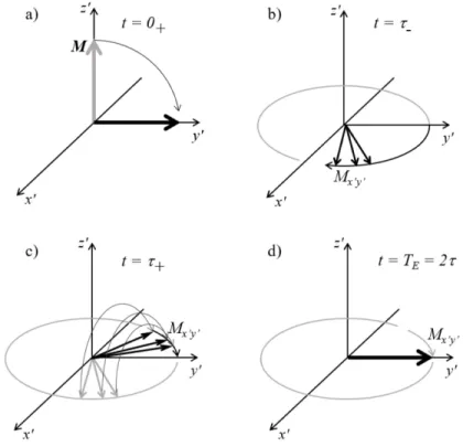
If a 90o_{RF pulse is followed by a 180}o_{RF separated by a time interval τ, a signal called spin echo}

can be generated. This scheme is called 90-τ-180 and it can be illustrated by the representations in Figure 2.8.

Figure 2.8 Evolution of the transverse magnetization due to a 90-τ-180 RF pulse sequence. The rotating frame is used and, for simplicity, only the evolution of Mx’y’ after the 90o pulse (t = 0+) is shown. A biological sample is initially placed in a B0 field which makes the net

magnetization M ideally aligned with the z’-axis. If a 90o_{RF pulse (𝛼𝛼}

1) is applied along the

x’-axis, M will be rotated to the y’-axis (a). After the pulse, M starts precessing around the z-axis and

Mxy describes a circle in the xy-plane. But in a real sample the inhomogeneities and the interactions among the spins make them precess in a range of frequencies instead of only at 𝜔𝜔0. This creates a

phase difference among the spins that progresses during the precession. In

Figure 2.8 (b) the Mx’y’ of some spins are shown. After a time τ, there will be a phase angle range ∆ωτ. If now a 180o_{pulse (𝛼𝛼}

2) is applied along the y’-axis, all the Mx’y’ will be flipped to the other

side of the x’y’-plane as shown in (c). As a result, the Mx’y’ that had the slower precession will be now ahead and the fastest ones behind. Since all the spins will continue precessing at the same frequencies and directions, after another time interval τ they will be all at the same phase as shown

(39)

in (d). In other words, after a t = TE = 2τ the phase coherence among the spins will be recovered. This rephasing process will generate a signal called echo. The maximum amplitude of this signal is given by [15]:

𝐴𝐴𝐸𝐸 = 𝑀𝑀𝑧𝑧0sin 𝛼𝛼1[sin(𝛼𝛼2⁄ )]2 2𝑒𝑒−𝑇𝑇𝐸𝐸⁄𝑇𝑇2 (2.21)

This expression shows the dependence on T2 of the echo signal and that the maximum is reached with the previous pulse combination, but it is lower than the FID. Figure 2.9 shows the evolution of the NMR signal with the explained RF pulse combination.

Figure 2.9 NMR signals due to a 90-τ-180 RF pulse sequence. Notice the 𝑇𝑇2∗ dependence of the

FID and the T2 dependence of the echo.

2.2.4 Signal detection

The NMR signal should be converted to an electrical signal to make it useful. Since the net magnetization is precessing at a radio frequency it can be captured by any conducting loop tuned at the same frequency by means of the Faraday law for electromagnetic induction. Taking advantage also of the principle of reciprocity [17] and after some mathematical treatment [15] the following expression for the voltage induced in a receiver loop, or coil, in the laboratory frame is found: 𝑉𝑉(𝑡𝑡) = � 𝜔𝜔(𝒓𝒓)�𝐵𝐵𝑟𝑟,𝑥𝑥𝑥𝑥(𝒓𝒓)��𝑀𝑀𝑥𝑥𝑥𝑥(𝒓𝒓, 0)� 𝑜𝑜𝑜𝑜𝑜𝑜𝑒𝑒𝑜𝑜𝑡𝑡 𝑒𝑒 −𝑡𝑡 𝑇𝑇⁄ 2(𝒓𝒓)cos�−𝜔𝜔(𝒓𝒓)𝑡𝑡 + ∅_𝑒𝑒(𝒓𝒓) − ∅𝑟𝑟(𝒓𝒓) + 𝜋𝜋 2� �𝑑𝑑𝒓𝒓 (2.22)

(40)

where r is a position in the laboratory frame, 𝜔𝜔(𝒓𝒓) is the free precession Larmor frequency, 𝑀𝑀𝑥𝑥𝑥𝑥(𝒓𝒓, 0) is the transverse magnetization and 𝐵𝐵𝑟𝑟,𝑥𝑥𝑥𝑥(𝒓𝒓) is the sensitivity of the coil determined by

the principle of reciprocity, all at the point r. ∅𝑟𝑟(𝒓𝒓) and ∅𝑒𝑒(𝒓𝒓) are respectively the reception phase

angle and the initial phase shift introduced by the excitation.

This RF signal is afterward demodulated by using a quadrature method based in phase-sensitive detection and power combination. The output of this demodulator is a complex signal expressed by [15]:

where:

𝛾𝛾∆𝐵𝐵(𝒓𝒓) = ∆𝜔𝜔(𝒓𝒓) (accounts for the inhomogeneity of B0 during the free precession) 𝐵𝐵𝑟𝑟,𝑥𝑥𝑥𝑥∗ (𝒓𝒓) = �𝐵𝐵𝑟𝑟,𝑥𝑥𝑥𝑥(𝒓𝒓)�𝑒𝑒−𝑖𝑖∅𝑟𝑟(𝒓𝒓)

𝑀𝑀𝑥𝑥𝑥𝑥(𝒓𝒓, 0) = �𝑀𝑀𝑥𝑥𝑥𝑥(𝒓𝒓, 0)�𝑒𝑒𝑖𝑖∅𝑒𝑒(𝒓𝒓)

2.2.5 Spatial encoding

An image can be reconstructed from NMR signals if spatial-dependent information is added. This is achieved by spatial encoding using magnetic field gradients. Three orthogonal gradient coil systems (x, y and z directions) are provided in the scanners with this purpose, as shown in Figure 2.1. Typically, the spatial encoding includes slice selection and both frequency and phase encoding. First, the spins in a sample need to be distinguished to enable slice selection. If a linear field gradient is added to the B0 field in one direction, for example z, the precession frequency of the spins will change in that direction. A selective RF pulse can now be configured, in shape and frequency, to excite a specific slice of the sample. In Figure 2.10 a) two possible slices, where protons precess at different Larmor frequencies, are shown. Since the NMR signal from the selected slice is a complex exponential, it can be spatially encoded while it is active by manipulating its frequency and its phase. With that purpose, two more gradients are added in the other two directions (x and y). Applying a linear gradient in the y direction will make the spins in that direction experience a different magnetic field and they will precess with different Larmor frequencies. After a certain time, a phase difference will be accumulated among them and the gradient is turned off as shown in Figure 2.10 (b). They will continue their precession around the z-axis at the frequency

𝑆𝑆(𝑡𝑡) = � 𝐵𝐵𝑟𝑟,𝑥𝑥𝑥𝑥∗

𝑜𝑜𝑜𝑜𝑜𝑜𝑒𝑒𝑜𝑜𝑡𝑡 (𝒓𝒓)𝑀𝑀𝑥𝑥𝑥𝑥(𝒓𝒓, 0)𝑒𝑒

(41)

they had before the gradient was applied (𝜔𝜔0), but the phase of the signal will contain spatial

information. This is called phase encoding. In this state, the spins aligned with the x-axis still have the same frequency. Thus, a new gradient must be added along the x-axis to make the Larmor frequency change in this direction. In consequence, this is called frequency encoding. The resultant NMR signal, which now is spatially encoded, can be processed to construct an MRI image by means of a 2D Fourier transform.

Figure 2.10 Spatial encoding. a) two possible selected slices on a human head having the Larmor frequency at the eyes and a higher frequency at the head. b) phase encoding reached by previously applying a time invariant frequency gradient Gy(t). All signals start with the same phase but at the end of the pulse they have a different phase. c) 3 x 3 matrix representing one selected slice from a) (the one at 𝜔𝜔0) where the phase-encoded signals from b) are subsequently

frequency-encoded by means of another time invariant frequency gradient (Gx(t)). Notice that each member of the matrix has a unique combination of phase and frequency.

The spatially encoded signal after detection can be expressed by [18]: 𝑆𝑆(𝑡𝑡) = � 𝜌𝜌(𝑥𝑥, 𝑦𝑦)

𝑜𝑜𝑜𝑜𝑜𝑜𝑒𝑒𝑜𝑜𝑡𝑡 𝑒𝑒

𝑖𝑖𝑖𝑖�𝐺𝐺𝑥𝑥𝑥𝑥+𝐺𝐺𝑦𝑦𝑥𝑥�𝑡𝑡_{𝑑𝑑𝑥𝑥𝑑𝑑𝑦𝑦} _(2.24)

where 𝜌𝜌(𝑥𝑥, 𝑦𝑦) is a spin distribution and 𝐺𝐺𝑥𝑥𝑥𝑥 and 𝐺𝐺𝑥𝑥𝑦𝑦 are the linear gradient fields at x and y. This

(42)

and 𝑘𝑘𝑥𝑥 = (−𝛾𝛾𝐺𝐺𝑥𝑥𝑡𝑡/2𝜋𝜋) can be made (for the FID). This transformation will map the time signal to

the known k-space signal [18]. Thus:

𝑆𝑆�𝑘𝑘𝑥𝑥, 𝑘𝑘𝑥𝑥� = � 𝜌𝜌(𝑥𝑥, 𝑦𝑦) 𝑜𝑜𝑜𝑜𝑜𝑜𝑒𝑒𝑜𝑜𝑡𝑡 𝑒𝑒

−𝑖𝑖2𝜋𝜋(𝑘𝑘𝑥𝑥𝑥𝑥+𝑘𝑘𝑦𝑦𝑥𝑥)𝑑𝑑𝑥𝑥𝑑𝑑𝑦𝑦 _(2.25)

x, 𝑘𝑘𝑥𝑥 and y, 𝑘𝑘𝑥𝑥 are then considered as the Fourier conjugate variables, as ω and t, which has the

same structure as a 2D Fourier integral. Then, taking the inverse Fourier transform of the detected signal will give the solution for the spin distribution 𝜌𝜌(𝑥𝑥, 𝑦𝑦) [18]:

In conclusion, when the inverse Fourier transform is applied to the raw data in k-space, an MRI image is obtained.

In general, not only constant gradients are used. They can also be a function of time, like a sinusoid for example. In those cases, the relationship between t and k should be written as: 𝑘𝑘(𝑡𝑡) =

𝑖𝑖

2𝜋𝜋∫ 𝐺𝐺(𝜏𝜏)𝑑𝑑𝜏𝜏 𝑡𝑡

0 [15].

2.2.6 Typical image acquisition sequence and k-space

Image sequences are composed by RF pulses and gradients conveniently combined to acquire images. The MR signals acquired with them are stored in k-space. One of the most important sequences, called Gradient Recalled Echo (GRE), is shown in Figure 2.11. In this sequence, the 180o_{RF pulse is replaced by gradient rephasing pulses. A 90}o_{RF pulse and a slice selection}

gradient Gz are simultaneously applied to tip M at a z position to the transverse plane. The negative part of Gz is used to re-phase the nuclei in the z direction which were de-phased by the positive part of Gz. After the negative Gz, a phase encoding gradient Gy is applied (red in Figure 2.11). This

creates a phase shift in the MR signal that is a function of the position in the y-direction. In k-space the magnetization is moved in the positive k-direction. A frequency or readout gradient, having a negative and a positive pulse, is applied after some delay (blue and green in Figure 2.11). The negative part (blue) is a previous compensation for the de-phasing that will create the positive part (green). The magnetization in k-space respectively moves to the negative x and to the positive x. As a result, the frequency of the MR signal is a function of the position in the x-direction. This gradient produces the echo signal as the transverse magnetization components re-phase gradually.

𝜌𝜌(𝑥𝑥, 𝑦𝑦) = 𝐹𝐹𝑇𝑇−1_{�𝑆𝑆(𝑘𝑘}

𝑥𝑥, 𝑘𝑘𝑥𝑥)� = � 𝑆𝑆(𝑘𝑘𝑥𝑥, 𝑘𝑘𝑥𝑥)

𝑘𝑘−𝑠𝑠𝑝𝑝𝑠𝑠𝑜𝑜𝑒𝑒 𝑒𝑒

(43)

The sequence is repeated, changing the amplitude of the phase gradient on each step, to move the magnetization to a new line in k-space until it is completely swept. Each line of k-space is filled with a digitized echo. The echo signal is recorded in quadrature, so each k-space point (black dots) is a complex number that contains spatial frequency and phase information about every pixel in the final image. For that reason, the inverse Fourier transform can convert k-space data in an MRI image.

Figure 2.11 Diagram of the Gradient Recalled Echo (GRE) pulse sequence and the trajectory of the magnetization in k-space.

The parameters of this sequence, namely the echo time (TE) and the repetition time (TR), along with the flip angle, are adjusted to modify the contrast of the images. This sequence is frequently used with small flip angles to reduce the scan times.

2.2.7 Signal to noise ratio (SNR)

The SNR is a very important parameter of the MRI images. It is typically measured as the ratio of the pixel intensity, or the mean inside a region of interest, and the standard deviation of the background noise. However, different methods and corrections are used according to the receiver coil and the experiment setup. The noise in NMR signal comes from spontaneous fluctuations such as the thermal motion of free electrons inside the electrical components and the sample that is being

(44)

scanned. This noise can be modified in the subsequent processing, which will have an impact on the image noise [15].

The SNR of the NMR signal depends on several variables that can be related by the following expression [17], [19]:

𝑆𝑆𝑁𝑁𝑆𝑆 ∝ 𝜔𝜔0𝐵𝐵02𝐾𝐾𝑉𝑉𝑠𝑠𝑠𝑠𝑠𝑠𝑝𝑝𝑠𝑠𝑒𝑒(𝐵𝐵1)𝑥𝑥𝑥𝑥

�4𝑘𝑘∆𝑓𝑓�𝑇𝑇𝑜𝑜𝑜𝑜𝑖𝑖𝑠𝑠𝑆𝑆𝑜𝑜𝑜𝑜𝑖𝑖𝑠𝑠+ 𝑇𝑇𝑠𝑠𝑠𝑠𝑠𝑠𝑝𝑝𝑠𝑠𝑒𝑒𝑆𝑆𝑠𝑠𝑠𝑠𝑠𝑠𝑝𝑝𝑠𝑠𝑒𝑒�

(2.27) where the numerator contains the signal-dependent variables and the denominator the noise-dependent variables. The signal depends on the static magnetic field B0, the geometry of the coil (𝐾𝐾 factor), the volume of the sample (𝑉𝑉𝑠𝑠𝑠𝑠𝑠𝑠𝑝𝑝𝑠𝑠𝑒𝑒) and the B1 components in the transverse plane (𝐵𝐵1+

related to the excitation field and 𝐵𝐵1− related to the sensitivity of the coil). The noise depends on

the reception bandwidth (∆𝑓𝑓), the temperature and the resistance of the coil and the sample; k is the Boltzmann constant. The main contribution to the noise at low B0 comes from 𝑆𝑆_{𝑜𝑜𝑜𝑜𝑖𝑖𝑠𝑠} while at higher fields it comes from 𝑆𝑆𝑠𝑠𝑠𝑠𝑠𝑠𝑝𝑝𝑠𝑠𝑒𝑒. This is because 𝑆𝑆𝑜𝑜𝑜𝑜𝑖𝑖𝑠𝑠 is proportional to √𝜔𝜔 due to the skin

effect while 𝑆𝑆𝑠𝑠𝑠𝑠𝑠𝑠𝑝𝑝𝑠𝑠𝑒𝑒 is proportional to 𝜔𝜔2.

2.2.8 Parallel imaging

The increase in SNR achieved with a phased array coil can be used to reduce the scan time by means of parallel imaging techniques. These techniques take advantage of the differences in the sensitivities of the array elements to reconstruct the images with reduced data. These differences can be used to create a sensitivity map of the coil that allows to determine the origin of a signal. The number of phase-encoding steps (k-space lines) is reduced by simultaneously acquiring data from multiple receive elements. This leads to reduced scan time and aliased images. Several methods were proposed for reducing the Fourier encoding, being Sensitivity Encoding (SENSE) one of the most established [20]. In this method, the SNR is reduced by at least √𝑆𝑆 due to the reduction of phase-encoding steps. R is defined as the factor by which the number of samples is reduced with respect to full Fourier encoding. Additional SNR losses are characterized by the g-factor (geometry g-factor) of the coil, which is always at least equal to one. The geometry g-factor describes the ability of the coil to separate pixels superimposed by aliasing. It allows a priori SNR estimates and provides an important criterion for the design of dedicated coil arrays since:

(45)

𝑆𝑆𝑁𝑁𝑆𝑆𝜌𝜌𝑟𝑟𝑒𝑒𝑟𝑟 = 𝑆𝑆𝑁𝑁𝑆𝑆𝜌𝜌 𝑟𝑟𝑓𝑓𝑠𝑠𝑠𝑠

𝑔𝑔𝜌𝜌√𝑆𝑆

(2.28)

where ρ is the index of the voxel under consideration, 𝑓𝑓𝑓𝑓𝑓𝑓𝑓𝑓 denotes full Fourier encoding and 𝑟𝑟𝑒𝑒𝑑𝑑 denotes reduced encoding.

2.3 Radiofrequency (RF) coils

As mentioned above RF coils can be divided in transmitter (Tx) coils, used to tip M from the z-axis, and receiver (Rx) coils, which are used to detect the signal induced by the precession of the spins. There is also a combination between them called transmitter/receiver (Tx/Rx) coils that is switched between both functions during the MRI experiment. Tx coils are desired to have a homogeneous B1 field while the Rx coils should have a high sensitivity and produce images with high SNR. The next sections will be focused mainly in surface Rx coils as they are the main topic of this work.

2.3.1 Coil model

An RF coil can be represented by a very simple series-resonant equivalent circuit, as shown in Figure 2.12. The resonance frequency of this circuit is the known expression: 𝜔𝜔 = 1 √𝐿𝐿𝐿𝐿⁄ . The signal from the sample and the noise are represented by VS and VN. R includes the coil losses (𝑆𝑆_{𝑜𝑜𝑜𝑜𝑖𝑖𝑠𝑠}) and the sample losses (𝑆𝑆𝑠𝑠𝑠𝑠𝑠𝑠𝑝𝑝𝑠𝑠𝑒𝑒). 𝑆𝑆𝑜𝑜𝑜𝑜𝑖𝑖𝑠𝑠 can be reduced by a proper selection of the coil materials

and dimensions. 𝑆𝑆𝑠𝑠𝑠𝑠𝑠𝑠𝑝𝑝𝑠𝑠𝑒𝑒 is the equivalent series resistance due to the induced eddy current losses

in the sample, which is a lossy conductor. It is related to the thermal motion of free electrons and it will always be present. Therefore, it is necessary to keep 𝑆𝑆𝑜𝑜𝑜𝑜𝑖𝑖𝑠𝑠 small compared to 𝑆𝑆𝑠𝑠𝑠𝑠𝑠𝑠𝑝𝑝𝑠𝑠𝑒𝑒 which

leads to the condition called sample noise dominance.