Numerical simulation of boiling during the quenching process

(1)

HAL Id: hal-00592676

https://hal.archives-ouvertes.fr/hal-00592676

Submitted on 3 May 2011

HAL is a multi-disciplinary open access archive for the deposit and dissemination of sci-entific research documents, whether they are pub-lished or not. The documents may come from teaching and research institutions in France or abroad, or from public or private research centers.

L’archive ouverte pluridisciplinaire HAL, est destinée au dépôt et à la diffusion de documents scientifiques de niveau recherche, publiés ou non, émanant des établissements d’enseignement et de recherche français ou étrangers, des laboratoires publics ou privés.

Numerical simulation of boiling during the quenching

process

Nadine Kosseifi, Elie Hachem, Luisa Silva, Séverine A.E. Boyer, Elisabeth

Massoni, Thierry Coupez

To cite this version:

Nadine Kosseifi, Elie Hachem, Luisa Silva, Séverine A.E. Boyer, Elisabeth Massoni, et al.. Numerical simulation of boiling during the quenching process. 10e colloque national en calcul des structures, May 2011, Giens, France. 8 p. ; Clé USB. �hal-00592676�

(2)

Numerical simulation of boiling during the quenching process

N. Kosseifi1, E.Hachem1, L. Silva1, S.A.E. Boyer2, E.Massoni1, T.Coupez1

1

Centre de Mise en Forme des Matériaux/ MINES ParisTech, 1 Rue Claude Daunesse, 06904 Sophia Antipolis Cedex, France

2 _{Département Physique et Mécanique des Matériaux / ENSMA-INSTITUT P’, 1 Avenue Clément Ader, 86961 Futuroscope Chasseneuil,}

France

Résumé — During the thermal modelling of the quenching process, different stages of boiling need to

be treated, from nucleate boiling to generation and growth of a vapour film. The interface between each phase flow is determined using a level set method. Surface tension is evaluated using the continuum surface force. The proposed approach demonstrates the capability of the model to simulate detachment of a single bubble and the generation of film vapour from a heated source. A comparison between numerical and experimental results shows a good agreement.

Mots clefs — Finite elements methods, quenching process, two-phase flow, bubble growth,

detachment, film vapour.

1 Introduction

The quenching process is an efficient way to control mechanical and metallurgical characteristics of final metallic parts. Nevertheless the heat transfer between the part and the quench fluid must be very well controlled to avoid defects like cracks, heterogeneous distribution of mechanical and metallurgical properties. The framework of this study is the improvement of the heat transfer knowledge between the solid part and the fluid thank to an innovative numerical description of the fluid behaviour at the interface and especially phase change (liquid, vapour) phenomenon of the cooling fluid.

During quenching, the metal temperature (Figure 1(a)) is higher than the fluid boiling temperature; consequently the fluid in the liquid state will be transformed in vapour as illustrated in Figure 1(b). The formation of bubble will remove temperature from the heated surface through vortex formation. Therefore, the nucleate boiling process is a very efficient mode of heat transfer and has a major role in the cooling process. Recently Srinivasan and al. [1] interpreted the boiling phase change within a quenching process by computing the heat flux that arises from the different modes of boiling. They coupled the phase change to heat dissipation of the metal thanks to an interface coupling code. The heat transfer coefficient depends on the positionand initial temperature of the solid, and bath agitation. To avoid such an empirical parameter and to simulate a general quenching process, in this work a single mesh for the solid and fluid domains is considered on which a set of global equations needs to be solved.

Different boiling modes prevail on the solid surface during the quenching process: film boiling, transition boiling and nucleate boiling. These modes are detailed in the paper of Bourouga and Gilles [2]. In order to better understand the boiling phenomena, the study of nucleate boiling behaviour is the first step. Nucleate boiling is considered as one of the most difficult challenges for direct simulation. The complexity remains in dealing numerically with the precision of the liquid-vapour interface. For computations of nucleate boiling, Son and Dhir [3] used a level set method to include the effect of phase change at liquid-vapour interface and to treat the no-slip condition. Welch and Wilson [4]

(3)

2 velocity deduced from the Gibbs Thomson relation, secondly the energy equation capable to take into account the latent heat as a source term, and finally the discretization of the Navier Stokes equations including the surface tension. Experimental and numerical study of the growth and detachment of a bubble from the heated plane surface are presented. The generation of vapour is also treated in section 4.

(a) (b)

Fig. 1 – (a) Quenching in water of a ferrule (SfarSteel-Areva, Creusot Forge). (b) Bubble generation during a micro quenching process (CEMEF-MINES ParisTEch, Sophia Antipolis).

2 Level set approach

Liquid vapour interface is defined by zero value of the level set function

φ

, which is the signed distance from the interface. The level set function

φ

is computed using a convected LevelSet method (Eq. 1), introduced and detailed in the works of Ville and al. [5]. The advantages of this method are: firstly, to restrict the convection resolution to the neighbourhood of the interface and secondly to

replace the reinitialisation steps by an advective reinitialisation. The distance function

φ

is truncated at a thickness

E

by a sinusoidal function denoted

α

which has the same zero value as the level set

φ

.

(

)

2 0 1 0 in 2 0, ( ) in u s t E t x x α _{α λ} _α π _α α α _∂  _ _   _{+ ⋅∇ +} _{∇ −} ₋ ₌ _Ω  _   _ ∂    _ _  = = Ω  Eq. 1

Here s is

α

sign,

λ

is chosen to be equal to

t

h

∆

and E=2h where h is the averaged mesh size in the vicinity of the interface.

The discontinuity of physical and thermodynamic properties at the interface may lead to oscillations and instabilities. Therefore the smoothed Heavisidefunction

H

(

φ

)

and a linear mixing law (Eq. 2) were used to define physical continuous properties.

( )

l

(

v l

) ( )

H ρ φ = +ρ ρ ρ− φ

Eq. 2

(4)

( )

0 if 1 1 1 sin if 2 1 if E H E E E E φ φ πφ φ φ π φ < −        =  + +   ≤       _>  Eq. 3

This part is devoted to the equations governing the bubble growth; conservation of mass, momentum, energy equations and Gibbs Thomson relation.

3 Governing equation

Let T_h(Ω)be the spatial discretization of the computational domain

Ω

. The unstructured Eulerian mesh is made of d-simplex elements K namely triangles in two dimensions (2D) and tetrahedral in three dimensions (3D), where d is the spatial dimension. The discretized domain, denoted Ωh, is defined as follows: ( ) h h K K ∈Τ Ω Ω =

U

Eq. 4

In the context of finite element method, a simple P1continuous approximation space V_h is chosen and defined by:

{

0 1

}

( ); ( ), ( ) h h h hK h V = v ∈C Ω v ∈P K ∀ ∈Τ ΩK Eq. 5 3.1 Interface velocity

Several experimental studies investigated by Zuber [6], Lee [7] and Qiu & Dhir [8] have been performed to compute the growth rate of bubbles in an infinite pool of liquid and at a heated surface. In both cases, the characteristic length R(t) varies as a function of the timet, the Jacob number Ja and the liquid thermal diffusivity al.

(

)

0 ( ) l n with l l w e v c T T R t C Ja a t Ja L ρ ρ ∗ − = = _{Eq. 6}

The authors in [9] determined

C

₀∗ and n as a function of the thermal parameters. In this numerical approach, to compute the interface growth velocity, the Gibbs Thomson relation is adopted as the works of Tan & Zabaras [10]. .

(

)

(

)

0 e 0 e

vr_Γ =C T−T nr_Γ=C T−T ∇α

Eq. 7

(5)

4 its contribution as an external force term as given in. (Eq. 8):

( )

(

( )

)

(

)

(

)

( )

0 in ( , 0) in ( , ) 0 in v l p v e v p l p dT d c k T L T T c c dt dt T T T t n φ ρ φ φ ρ ρ ρ δ φ_Γ  _ _ − ∇⋅ ∇ = − + − − Ω     = Ω  _∇ _{⋅ =} _∂Ω   x x r Eq. 8

L

is the latent heat of vaporisation per unit mass, T_e is the boiling temperature. The smoothed delta function

δ

_Γ is given by Croce [11] as the derivative of smoothed heaviside function:

( )

0 1 1 cos 2 if E H if E E E φ φ δ φ φ _πφ φ Γ  _>  = ∂ =    +   <         Eq. 9

3.3 Incompressible navier-stokes equations

The behaviour of fluids is governed by the Navier Stokes equations defined on the domain

Ω

. In several applications that belong to the phase flow problems, surface tension plays a dominant role in defining the bubble’s shape. The surface tension is presented at the interface of two fluids when at least one of them is liquid.

Van der Pijl [12] presents the surface tension as a volume forceF_V = _Γnr_Γ

r

σκδ

ρ

1

. It wasincluded by Croce [11] as a source term in the Navier Stokes equations with variable densities as follows in (Eq. 10):

( )

(

( )

(

)

( )

₍

_{( )}

₎

in 0 in 0 in T du u u p g kn dt d u dt u σ ρ φ µ φ ρ φ δ φ ρ ρ φ _{ρ φ} Γ Γ    − ∇ ⋅ ∇ + ∇ + ∇ = + Ω        + ∇⋅ = Ω   = ∂Ω    r Eq. 10

Here, u is the velocity,

p

is the pressure and

g

is the constant gravity field. The parameter

σ

is the surface tension coefficient and

ρ

is the average density given by

(

)

2

1

1 0

ρ

=

+

. The

advantage of this method is that intrinsic geometric properties of the front may be easily determined from the level setfunction. For example, at any point the normal vector nr_Γand the mean curvature k, are given in

and

nr_Γ = ∇φ k= −∇ ⋅nr_Γ

Eq. 11

The computation of the surface tension force by using the continuum surface force (CSF) depends on the location and the derivatives of the interface. The main challenge in this approach is to compute

(6)

the curvature of the fluid interface as a second derivative of the Level set function since a linear finite element method is used. In this paper, we use a new method to compute the gradient directly at the nodes of the mesh presented in Coupez [13]. It is well known that the classical finite element approximation for the flow problem may fail because of two reasons: the compatibility condition known as the inf-sup condition and when the convection dominates. Therefore, a recently developed stabilised finite element method is used to discretize Navier Stokes equations depicted in [14].

4 Model validation

.

4.1 Bubble growth and detachment

4.1.1 Experimental study

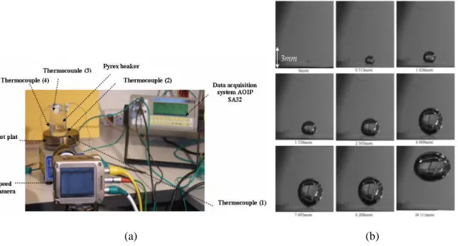
In the present study, we report a detailed study of a single bubble growth, shape and departure on a heated surface. Nucleate boiling experiment is performed using distilled water. The aim of this experiment is to compute the bubble growth rate. A schematic diagram of the experimental apparatus used in this study is shown in Figure 2(a). The beaker is made of a Pyrex glass; it has an inner diameter of 35.55 mm, a thickness of 6.2 mm and a height of 6 cm. The beaker is filled with 20ml of distilled water. Images of bubble growth were captured using a high speed camera (Phantom Miro eX-series) Photonetics (125 to 2500 images/s) and coupled with a 110 macro photos objective. Figure 2(b) shows that the bubble has a hemispherical or oblate shape at the early growth stage then it changes to an elongated shape as it proceeds towards the detachment. After the bubble breaks away, a second nucleus is possibly developed.

(a) (b)

Fig. 2 – (a) Experimental apparatus. (b) Experimental studies for comparison.

(7)

6 and the vapour to be superheated at a temperature of

103 °

C

. The fluid temperature increases linearly from the heated wall.

The computational domain is a cube of

7 mm

side, discretized using an 100×100×100 unstructured

grid mesh. The bubble having initial radius

R

=

0 .

5 mm

has been placed at the centre bottom next to the wall as illustrated in the top of Figure 3. We consider a two-phase fluid with surface tension

1 . 1 . 0 − = Nm

σ

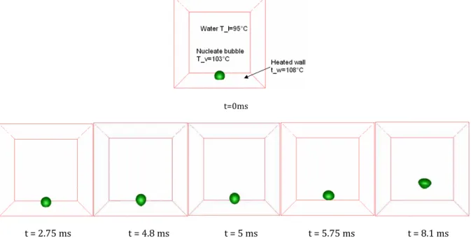
, a latent heat L=88000 j.kg−1and a constant gravityg =9.81m.s−1. The transport velocity is the result of the sum of the fluid velocity solution of Navier-Stokes equation and the given growth velocityvr_Γ =0.024(T−T_e)nr_Γ.

The fluid properties, including density and viscosity are assumed to be constant in each phase it corrempond to liquid and vapour phase. During the ascension, the form of the bubble changes to an elongated spheroid while its growth is not significant. Figure 3 shows the bubble detachment from an heated surface. After the detachment, the bubble shape changes depending on the surface tension from spherical to an oval shape (bottom row).

t=0ms

t = 2.75 ms t = 4.8 ms t = 5 ms t = 5.75 ms t = 8.1 ms

Fig. 3 – Isovalue zero of the level set function (positioning the liquid-vapour interface) for a three-dimensional nucleate boiling simulation.

4.2 Vapour generation- film boiling

The aim of this test is to bring out the generation of a vapour film around a solid object, close to the quenching problem. Therefore, we use a heat source to warm the surrounding liquid. As the growth velocity is proportional to the temperature difference, the vapour will appear when the liquid temperature is higher than the boiling temperature. Since the physical properties such as density and viscosity differ from one phase to another, the level set function has been used to separate the vapour film of the surrounding liquid allowing a mix of their properties and to track the interface. The film boiling mode occurs when the solid temperature is higher than the Leindenfrost point. The duration and the stability of the film boiling mode increase linearly with the growth of the bath temperature [15]. This boiling mode is the most noted for a bath having a temperature above

60 °

C

. Therefore we consider the water initially at a temperature of

90 °

C

.

(8)

This computation is performed in a three-dimensional hexahedral domainΩ=

[

0.15,0.06,0.2

]

m3. The heat source having the following dimensions

[

0.02,0.02,0.08

]

m3 is located at

)

06 .

0 ,

02 .

0 ,

065 .

0 (

as illustrated in Figure 4(a). The heat source is made of Inconel-718 at a temperature of

700 °

C

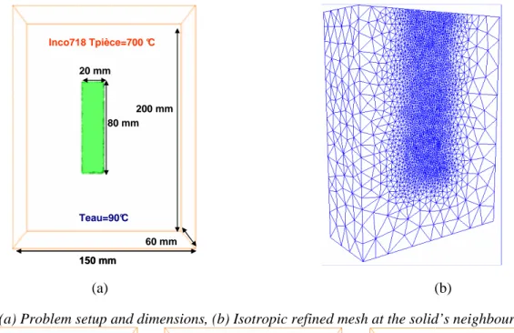
. The vapour interface is initially coincident with the solid’s boundary. In this test, the constant growth velocity isC₀ =0.00025. At the solid neighbourhood an isotropic refined mesh is used (h=0.0012), whereas the rest of domain kept the same background sizeh=0.025

h=0.025 as illustrated in Figure 4(b).

As shown in Figure 5, a continuous vapour layer forms between the heated solid and the surrounding liquid. The vapour is removed on the upper portion of the solid, which is determined by Taylor instability. From this test we can deduce that in the quenching process the dipped metal provide a natural generator of vapour.

(a) (b)

Fig. 4 – (a) Problem setup and dimensions, (b) Isotropic refined mesh at the solid’s neighbourhood

t = 0.2 s t = 0.25 s t = 0.375 s 150 mm 200 mm 80 mm 20 mm Teau=90°C Inco718 Tpièce=700 °C 60 mm 150 mm 200 mm 80 mm 20 mm Teau=90°C Inco718 Tpièce=700 °C 60 mm

(9)

8

5 Conclusion

A novel numerical approach is presented for the simulation of phase change by using the level set method to track the interface liquid-vapour and by solving one set of equations in both domains with different phase properties. To simulate multi phase flows where the fluids are considered to be incompressible, the surface tension was computed bycontinuum surface force CSF method.

The numerical three dimensional (3D) tests show that the proposed method is able to simulate the phase change during the quenching process. This method takes advantage of the level set method to capture the interface and avoid the complexity to take into account the heat transfer for the different boiling modes. The application of this approach in a 3D test shows the evolution of the bubble shape during the detachment from a heated wall. This method was also applied to simulate the generation of a film of vapour followed by its detachment. Further experimental work is in progress to obtain details about velocity and temperature in the surrounding flow field by applying Particle Image Velocimetry and Planar Laser Induced Fluorescence (PIV-PLIF). The growth constant will then be specified, by comparing numerical and experimental results.

Acknowledgement

The authors present their acknowledgements to the CIM Team (Calcul Intensif en Mise en Forme) and the companies involved in the THOST (Thermal Optimisation System) project managed by Science Computer and Consultants (SCC).

References

[1] V. Srinivasan, K. Moon, D. Greif , D. M. Wang, M. Kim. Numerical simulation of immersion quenching process of an engine cylinder head. Applied Mathematical Modelling, 34: 2111-2128, 2010.

[2] B. Bourouga, J. Gilles. Roles of heat transfer modes on transient cooling by quenching process,

International Journal Mater Form, Original Research, 10.1007/s12289-009-0645-z, 2009.

[3] G. Son, V.K. Dhir. Numerical simulation of nucleate boiling on a horizontal surface at high heat fluxes.

International Journal of heat and Mass transfer, 51: 2566-2582, 2008.

[4] S. Welch, J. Wilson. A volume of fluid based method for fluid flow with phase change. Journal of

computational physics, 160: 662,682, 2000.

[5] L. Ville, L. Silva, T. Coupez. Convected level set method for the numerical simulation of fluid bulking.

International Journal for numerical methods in fluids, article in press, 2010, doi: 10.1002/fld.2259.

[6] N. Zuber. The dynamics of vapour bubbles in nonuniform temperature field. International Journal of Heat

and Mass Transfer, 2: 83-98, 1961.

[7] H. Lee, B. Oh , S. Bae, M. Kim. Single bubble growth in saturated pool boiling on a constant wall temperature surface; International Journal of Multiphase Flow, 29:1857-1874, 2003.

[8] D. Qiu, V.K. Dhir. Experimental study of flow pattern and heat transfer associated with a bubble sliding on

downward facing inclined surfaces. Experimental Thermal and Fluid Science, 26: 605-616, 2002.

[9] M. Barthès. Ebullition sur site isolé étude expérimentale de la dynamique de croissance d’une bulle et des

transferts associés. Ph.D. Thesis, Université De Provence, 2005.

[10] L. Tan, N. Zabaras. A level set simulation of dendritic solidification with combined features of front- tracking and fixed-domain methods. Journal of computed physics, 211: 36-63, 2006.

[11] R. Croce, M. Griebel, Al. Schweitzer. Numerical simulation of bubble and droplet deformation by a level

set approach with surface tension in three dimensions. International Journal for numerical methods in

fluids, 62: 963-993, 2010.

[12] S. P. van der Pijl, A. Segal, C. Vuik, P. Wesseling. A mass-conserving Level-Set method for modelling of

multi-phase flows; International journal for numerical methods in fluids, 47:339–361, 2005.

[13] T. Coupez. Metric construction by length distribution tensor and edge based error for anisotropic adaptive meshing, article in press, Journal of computational physics, 2010

[14] E. Hachem, B. Rivaux, T. Kloczko, H. Digonnet, T. Coupez, Stabilized finite element method for

incompressible flows with high Reynolds number, Journal of Computational Physics, Volume 229, Issue 23, 2010, Pages 8643-8665, DOI: 10.1016/j.jcp.2010.07.030.

[15]G. Jérome. Etude Expérimentale des Aspects Thermiques lies à une Opération de Trempe. Ph.D. Thesis,