HAL Id: hal-00456549
https://hal.archives-ouvertes.fr/hal-00456549
Submitted on 15 Feb 2010
HAL is a multi-disciplinary open access
archive for the deposit and dissemination of
sci-entific research documents, whether they are
pub-lished or not. The documents may come from
teaching and research institutions in France or
abroad, or from public or private research centers.
L’archive ouverte pluridisciplinaire HAL, est
destinée au dépôt et à la diffusion de documents
scientifiques de niveau recherche, publiés ou non,
émanant des établissements d’enseignement et de
recherche français ou étrangers, des laboratoires
publics ou privés.
Model-Driven Constraint Programming
Raphael Chenouard, Laurent Granvilliers, Ricardo Soto
To cite this version:
Raphael Chenouard, Laurent Granvilliers, Ricardo Soto. Model-Driven Constraint Programming.
International Conference on Principles and Practice of Declarative Programming, Jul 2008, Valence,
Spain. pp.236-246, �10.1145/1389449.1389479�. �hal-00456549�
Model-Driven Constraint Programming
Rapha¨el Chenouard
CNRS, LINA, Universit´e de Nantes, France.
Laurent Granvilliers
CNRS, LINA, Universit´e de Nantes, France.
Ricardo Soto
CNRS, LINA, Universit´e de Nantes, France.
Pontificia Universidad Cat´olica de Valpara´ıso, Chile.
Abstract
Constraint programming can definitely be seen as a model-driven paradigm. The users write programs for modeling problems. These programs are mapped to executable models to calculate the solu-tions. This paper focuses on efficient model management (defini-tion and transforma(defini-tion). From this point of view, we propose to revisit the design of constraint-programming systems. A model-driven architecture is introduced to map solving-independent con-straint models to solving-dependent decision models. Several im-portant questions are examined, such as the need for a visual high-level modeling language, and the quality of metamodeling tech-niques to implement the transformations. A main result is the s-COMMAplatform that efficiently implements the chain from mod-eling to solving constraint problems.
Categories and Subject Descriptors D.3.2 [Programming
Lan-guages]: Language Classifications—Constraint and logic
lan-guages; D.2.2 [Software Engineering]: Design Tools and Tech-niques—User interfaces; D.3.3 [Programming Languages]: Lan-guage Constructs and Features—Classes and objects, Constraints
General Terms Languages
Keywords Constraint Modeling Languages, Constraint Program-ming, Metamodeling, Model Transformation
1.
Introduction
In constraint programming (CP), programmers define a model of a problem using constraints over variables. The variables may take values from domains, typically boolean, integer, or rational values. The solutions to be found are tuples of values of the variables satis-fying the constraints. The search process is performed by powerful solving techniques, for instance backtracking-like procedures and consistency algorithms to explore and reduce the space of potential solutions. In the past, CP has been shown to be efficient for solving hard combinatorial problems.
CP systems evolved from the early days of constraint logic pro-gramming (CLP). In a CLP system, the constraint language is em-bedded in a logic language, and the solving procedure combines the SLD-resolution with calls to constraint solvers [15]. The logic lan-guage can be replaced with any computer programming lanlan-guage
Permission to make digital or hard copies of all or part of this work for personal or classroom use is granted without fee provided that copies are not made or distributed for profit or commercial advantage and that copies bear this notice and the full citation on the first page. To copy otherwise, to republish, to post on servers or to redistribute to lists, requires prior specific permission and/or a fee.
PPDP’08, July 16–18, 2008, Valencia, Spain.
Copyright c 2008 ACM 978-1-60558-117-0/08/07. . . $5.00
(e.g. C++ in ILOG Solver [26] or Java in Gecode/J [12]) and even term rewriting [11]. It turns out that the programming task may be hard, especially for non experts of CP or computer programming. In this approach, modeling concerns are not enough to write pro-grams, and it is often mandatory to deal with the encoding aspects of the host language or to tune the solving strategy. In response to this problem, almost pure modeling languages have been built, such as OPL [30] and Zinc [27].
The design of the last generation of CP systems has been gov-erned by the idea of separating modeling and solving capabilities (e.g. Essence [9] and MiniZinc [21]). The system architecture has three layers, including the modeling language, the solvers, and a middle tool composed by a set of solver-translators implementing the mappings. In particular, this approach gives important bene-fits: The full expressiveness of CP is supported by a unique high-level modeling language, which is expected to be simple enough for non experts. The user is able to process one model with different solvers, a crucial feature for easy and fast problem experimentation. The platform is open to plug new solvers.
Our work follows this solver-independent idea, but under a Model-Driven Development (MDD) approach [24], which is well-known in the software engineering sphere. General requirements have been defined for MDD architectures in order to define concise models, to enable interoperability between tools, and to easily pro-gram mappings between models. The classical MDD infrastructure uses as base element the notion of a metamodel, which allows one to clearly define the concepts appearing in a model.
In this paper, the MDD approach is applied to a CP system. The goal is to implement the chain from modeling to solving con-straints. Our approach is to transform user solving-independent models defined through a visual modeling language to solver (ex-ecutable) models using a metamodeling strategy. CP concepts like domains, variables, constraints, and relations between them are de-fined in a metamodel, and thus the transformation rules are able to map these concepts from a source language to a target one. It results in a flexible and extensible architecture, robust enough to support changes at the mapping tool level. Moreover, we believe that the study of metamodels for CP is of interest.
These ideas have been implemented in the s-COMMA
plat-form [28]. The front tool allows users to graphically define straint models. It is made on top of a general object-oriented con-straint language [29]. Many solvers have been plugged in the plat-form such as ECLiPSe[31], Gecode/J [12], GNU Prolog [6] and Realpaver [14]. Upgrades are supported at the mapping tool, new solver-translators can be added by means of the AMMA plat-form [20].
The language for stating constraints ins-COMMAis clearly not the novel part of the platform, in fact it includes typical and state-of-the-art modeling constructs and features. Novelty arises from
the introduction of a solver-independent visual language – which we believe is intuitive and simple enough for non experts –, and the use of a MDD approach involving metamodeling techniques to implement the mappings.
The outline of this paper is as follows. The MDD architecture proposed is introduced in Section 2. Thes-COMMAmodeling
lan-guage and the associated graphical interface are presented in Sec-tion 3. The mapping tool and the metamodeling techniques used to develop solver-translators are explained in Section 4. Some exper-imental results are then discussed in Section 5. The related work and conclusion follows.
2.
A MDD approach for CP
Model-Driven Engineering (MDE) aims to consider models as first class entities. A model is defined according to the semantics of a model of models, also called a metamodel. A metamodel describes the concepts appearing in a model, but also the links between these concepts, such as: inheritance, composition or simple association.
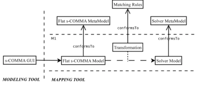
Figure 1 depicts a general Model-Driven Architecture (MDA) for model transformation. Level M1 holds the model. Level M2 describes the semantic of the level M1 and thus identifies concepts handled by this model through a metamodel. Level M3 is the specification of level M2 and is self-defined. Transformation rules are defined to translate models from a source model to a target one, the semantic of these rules is also defined by a metamodel.
A major strength of using this metamodeling approach is that models are concisely represented by metamodels. This allows one to define transformation rules that only operate on the concepts of metamodels (at the M2 level of the MDA approach), not on the concrete syntax of a language. Syntax concerns are defined independently (we illustrate this in Section 4). This separation is a great advantage for a clearly definition of transformation rules and grammar descriptions, which are the base of our mapping tool.
Figure 1. A general MDA for model transformation.
Let us now illustrate how this approach is implemented in our platform. Figure 2 shows the MDDs-COMMAarchitecture, which is composed by two main parts, a modeling tool and a mapping tool.
Thes-COMMA GUIis our modeling tool, and it allow users to
state constraint models using visual artifacts. An exactly textual representation of this language is also provided (for who does not want to use visual artifacts). Both languages are solver-independent and are designed conform to the same metamodel (see Section 3). The output of thes-COMMA GUIisFlat s-COMMAan
interme-diate language which is still solver-independent but, in terms of abstraction is closer to the solver level. The goal is to simplify the development of solver-translators.Flat s-COMMAis also designed conform to a metamodel (see Section 3.3).
The mapping tool is composed by a set of solver-translators. Solver-translators are designed to match the metamodel concepts ofFlat s-COMMAto the concepts of the solver metamodel (see
Section 4). This process is defined conform to the general MDA for model transformation.
Figure 2. The MDD architecture of s-COMMA.
Thes-COMMA GUIis written in Java (about 30000 lines) and
translators are developed using the AMMA platform. The whole system allows to perform the complete process from visual models to solver models. The system involves several metamodels: an s-COMMA metamodel, a Flat s-COMMAand solver metamodels.
The s-COMMA metamodel has been built just for defining the
concepts of thes-COMMA textual and visual language, it is not used to maps-COMMAtoFlat s-COMMA. For this task we already have an efficient translator. Our key aim of using metamodeling techniques is to provide an easier way to develop new solver-translators, compared to the task of writing translators by hand.
In the following two sections we present the main parts of this architecture: The modeling and the mapping tool, respectively.
3.
Modeling Tool
We have built ours-COMMA GUImodeling tool on top of the s-COMMAlanguage. Thes-COMMAlanguage is defined through its metamodel and it has been designed to represent the concepts of constraint problems, also called constraint satisfaction problems (CSPs). In this metamodel, the CSP concepts such as variables and domains have been merged with object-oriented concepts in order to state CSPs using an oriented style. The result is an object-oriented visual language for modeling CSPs. These decisions are supported by the following benefits:
• A problem is generally composed of several parts which may represent objects. They are naturally specified through classes. Thus, we obtain a more modular model, instead of forcing modelers to state the entire problem in a single block of code.
• We gain similar benefits – constraint and variable encapsula-tion, composiencapsula-tion, inheritance, reuse – to those gained by writ-ing software in a object-oriented programmwrit-ing language.
• Visual artifacts are more intuitive to use and give a clearer view of the complete structure of the problem.
Figure 3 illustrates the main concepts of thes-COMMA meta-model using UML class diagram notation. The role of each one of these concepts is explained in the following paragraphs.
3.1 s-COMMA models
Thes-COMMA metamodel defines the concepts appearing in s-COMMAmodels. Thus, conform to this metamodel ans-COMMA
model must be composed by two main parts, the model and data. The model describes the structure of the problem and the data con-tain the constant values used by the model. In ours-COMMA GUI
and the data concept is represented by the data artifact1(see Fig-ure 4).
Figure 3. s-COMMA Metamodel.
3.1.1 Class artifacts
Class artifacts have by default three compartments, the upper com-partment for the class name, the middle comcom-partment for attributes and the bottom one for constraint zones. By clicking on the class artifact its specification can be opened to define its class name, their attributes and constraint zones. Relationships can be used to define inheritance (a subclass inherits all attributes and constraint zones of its superclass) or composition between classes.
3.1.2 Data artifacts
Data artifacts have two compartments, one for the file name and another for both the constants and variable-assignments. Constants, also called data variables can be defined with a real, integer or enu-meration type. Arrays of one dimension and arrays of two dimen-sions of constants are allowed. Variable-assignment corresponds to the assignment of a value to a variable of an object. Variable-assignments can also be performed if objects are inside an array (see an example in Section 3.2).
Figure 4. Class artifact used in s-COMMA GUI
1Artifacts used on the s-COMMA GUI have been adapted from the class artifact provided by the UML Infrastructure Library Basic Package. This adaptation is completely allowed by the UML Infrastructure Specifica-tion [23].
3.1.3 Attributes
Attributes may represent decision variables, sets, objects or arrays. Decision variables can be defined by an integer, real or boolean type. Sets can be composed of integers or enumeration values. Objects are instances of classes which must be typed with their class name. Arrays of one and two dimensions are allowed, they can contain decision variables, sets or objects. Decision variables, sets and arrays can be constrained to a determined domain.
3.1.4 Constraint Zones
Constraint zones are used to group constraints encapsulating them inside a class. A constraint zone is stated with a name and it can contain the following elements:
• Constraints: Typical operations and relations are provided
to post constraints. For example, comparison relations (<,>, <=,>=,=,<>), arithmetic operations (+,*, -,/), logical re-lations (and,or,xor, ->,<-,<->), and set operations (in, subset, superset, union, diff, symdiff, intersection, cardinality).
• Statements: Forall and conditional statements are supported.
The forall (e.g.forall(i in 1..5)) is stated by declaring a loop-variable (i) and the set of values to be traversed (1..5). A loop-variable is a local variable and it is valid just inside the loop where it was declared. Conditionals are stated by means of if-else expressions. For instance,if(a) b else c;whereais the condition, which can includes decision variables; andband
care the alternatives, which may be statements or constraints.
• Objective: objective functions are allowed and they can be
stated by tagging the expression involved with the selected option (e.g.[minimize] x+y+z;).
• Global Constraints: a basic set of global constraints (e.g.
alldif-ferent, cumulatives) is supported. Additional constraints can be integrated to this basic set by means of extension mechanisms (for details refer to [29]).
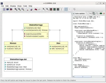
3.2 The stable marriage problem
Let us now illustrate some of these concepts in thes-COMMA GUI
by means of the stable marriage problem.
Figure 5. The stable marriage problem on the s-COMMA GUI
Consider a group of n women and a group of n men who must marry. Each women has a preference ranking for her possible hus-band, and each men has a preference ranking for his possible wife.
The problem is to find a matching between the groups such that the marriages are stable i.e., there are no pair of people of opposite sex that like each other better than their respective spouses.
Figure 5 shows a snapshot of thes-COMMA GUI where the
stable marriage problem is represented by a class diagram. This diagram is composed by three classes, one class to represent men, one to represent women, and a main class to describe the stable marriages. Once the user states a visual artifact, the corresponding
s-COMMAtextual version is automatically generated on the
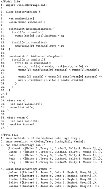
right-panel of the tool. For readability we illustrate the textual version of the problem in Fig. 6
//Model file 1. import StableMarriage.dat; 2. 3. class StableMarriage { 4. 5. Man man[menList]; 6. Woman woman[womenList]; 7. 8. constraint matchHusbandWife { 9. forall(m in menList) 10. woman[man[m].wife].husband = m; 11. 12. forall(w in womenList) 13. man[woman[w].husband].wife = w; 14. } 15. 16. constraint forbidUnstableCouples { 17. forall(m in menList){ 18. forall(w in womenList){ 19. man[m].rank[w] < man[m].rank[man[m].wife] -> 20. woman[w].rank[woman[w].husband] < woman[w].rank[m]; 21. 22. woman[w].rank[m] < woman[w].rank[woman[w].husband] -> 23. man[m].rank[man[m].wife] < man[m].rank[w]; 24. } 25. } 26. } 27.} 28. 29. class Man { 30. int rank[womenList]; 31. womenList wife; 32. } 33. 34. class Woman { 35. int rank[menList]; 36. menList husband; 37. } //Data file
1. enum menList := {Richard,James,John,Hugh,Greg}; 2. enum womenList := {Helen,Tracy,Linda,Sally,Wanda}; 3. Man StableMarriage.man :=
[Richard: {[Helen:5 ,Tracy:1, Linda:2, Sally:4, Wanda:3],_}, James : {[Helen:4 ,Tracy:1, Linda:3, Sally:2, Wanda:5],_}, John : {[Helen:5 ,Tracy:3, Linda:2, Sally:4, Wanda:1],_}, Hugh : {[Helen:1 ,Tracy:5, Linda:4, Sally:3, Wanda:2],_}, Greg : {[Helen:4 ,Tracy:3, Linda:2, Sally:1, Wanda:5],_}];
4. Woman StableMarriage.woman :=
[Helen: {[Richard:1, James:2, John:4, Hugh:3, Greg:5],_}, Tracy: {[Richard:3, James:5, John:1, Hugh:2, Greg:4],_}, Linda: {[Richard:5, James:4, John:2, Hugh:1, Greg:3],_}, Sally: {[Richard:1, James:3, John:5, Hugh:4, Greg:2],_}, Wanda: {[Richard:4, James:2, John:3, Hugh:5, Greg:1],_}];
Figure 6. An s-COMMA model for the stable marriage problem.
The class representing men (at line 29 in the model file) is composed by one array containing integer values which represents the preferences of a man, the array is indexed by the enumeration typewomenList(at line 2 in the data file), thereby the 1st index of the array is Helen, the 2nd is Tracy, the third is Lindaand so on. Then, an attribute calledwife is defined (line 31), which
represents the spouse of an object man. This variable haswomenList
as a type which means that its domain is given by the enumeration
womenList. The definition of the classWomenis analogous. The classStableMarriagehas a more complex declaration. We first define two arrays, one calledmanwhich contains objects of the classManand other which contains objects of the classWoman. Each one represents the group of men and the group of women, respectively. The composition relationship between classes can be seen on the class diagram.
At line 8 a constraint zone calledmatchHusbandWifeis stated. In this constraint zone, twoforall loops including a constraint are posted to ensure that the pairs man-wife match with the pairs woman-husband. The forbidUnstableCouples constraint zone contains two loops including two logical formulas to ensure that marriages are stable.
The data file is called by means of an import statement (at line 1). This file contains two enumeration types, menList and
womenList, which have been used in the model as a type, for in-dexing arrays, and as the set of values that loop-variables must tra-verse.StableMarriage.man is a variable-assignment for the array calledmandefined at line 5 in the model file.
This variable-assignment is composed by five objects (enclosed by‘{}’), one for each men of the group. Each of these objects has two elements, the first element2 is an array (enclosed by‘[ ]’).
This array sets the preferences of a men, assigning the values to the arrayrankof aManobject (e.g. Richard prefers Tracy 1st, Linda 2nd, Wanda 3rd, etc).
The second element is an underscore symbol (’ ’). This symbol is used to omit assignments, so the variable wife remains as a decision variable of the problem i.e., a variable for which the solver must search a solution.
3.3 Flat s-COMMA models
Before explaining how s-COMMA models are mapped to their
equivalent solver models, let us introduce the intermediateFlat s-COMMAlanguage.
Figure 7. Flat s-COMMA Metamodel.
Flat s-COMMAhas been designed to simplify the transforma-tion process froms-COMMAmodels to solver models. InFlat s-COMMAmuch of the constructs supported bys-COMMAare trans-formed to simpler ones, in order to be closer to the form required by classical solver languages.Flat s-COMMAis also defined by a metamodel.
Figure 7 illustrates the main elements of the Flat s-COMMA
metamodel, where manys-COMMAconcepts have been removed.
Now, the metamodel is mainly a definition of a problem composed by variables (decision variables) and constraints.
In order to transforms-COMMAtoFlat s-COMMA, several steps
are involved, which are explained in the following.
2Let us note that we use standard modeling variable-assignments, that is, assignments are performed respecting the order of the class’ attributes: the first element of the variable-assignment is matched with the first attribute of the class, the second element of the variable-assignment with the second attribute of the class and so on.
•Enumeration substitution: In general solvers do not support non-numeric types. So, enumerations are replaced by integer values. However, enumeration values are stored to show the results in the correct format.
•Data substitution: Data variables stated in the model file are replaced by their corresponding values i.e., the value defined in the data file.
•Loop unrolling: Loops are not widely supported by solvers, hence we generate an unrolled version of the forall loop.
•Flattening composition: The hierarchy generated by composi-tion is flattened. This process is done by expanding each object declared in the main class adding its attributes and constraints in theFlat s-COMMAfile. The name of each attribute has a pre-fix corresponding to the concatenation of the names of objects of origin in order to avoid name redundancy.
•Conditional removal: Conditional statements are transformed to logical formulas. For instance,if a then b else cis replaced by(a ⇒ b) ∧ (a ∨ c).
•Logic formulas transformation: Some logic operators are not supported by solvers. For example, logical equivalence (a ⇔
b) and reverse implication (a ⇐ b). We transform logical
equivalence expressing it in terms of logical implication ((a ⇒ b) ∧ (b ⇒ a)). Reverse implication is simply inverted (b ⇒ a).
1. variables: 2. 3. womenList man_wife[5] in [1,5]; 4. menList woman_husband[5] in [1,5]; 5. 6. constraints: 7. 8. woman_husband[man_wife[1]]=1; 9. woman_husband[man_wife[2]]=2; 10. woman_husband[man_wife[3]]=3; 11. ... 12. 13. man_wife[woman_husband[1]]=1; 14. man_wife[woman_husband[2]]=2; 15. man_wife[woman_husband[3]]=3; 16. ... 17. 18. 5<man_1_rank[man_wife[1]] -> 19. woman_1_rank[woman_husband[1]]<1; 20. 1<woman_1_rank[woman_husband[1]] -> 21. man_1_rank[man_wife[1]]<5; 22. 23. 1<man_1_rank[man_wife[1]] -> 24. woman_2_rank[woman_husband[2]]<3; 25. 3<woman_2_rank[woman_husband[2]] -> 26. man_1_rank[man_wife[1]]<1; 27. ... 28. 29. enum-types: 30. 31. menList := {Richard,James,John,Hugh,Greg}; 32. womenList := {Helen,Tracy,Linda,Sally,Wanda};
Figure 8. The Flat s-COMMA model of the stable marriage
prob-lem.
Figure 8 depicts theFlat s-COMMAmodel of the stable
mar-riage problem. The file is composed of two main parts, variables and constraints. Variables at lines 3-4 are generated by the flatten-ing composition process. The array mancomposed by objects of typeManis decomposed and transformed to a single array of deci-sion variables. The arrayman wifecontains the decision variables
wifeof the original arrayman; and the arraywoman husband con-tains the decision variableshusbandof the original arraywoman. The arrays rank of both objectsManandWomanare not considered as de-cision variables since they have been filled with constants (at lines
3-4 of the data file in Figure 6). The size of the arrayman wifeis 5, this value is given by the enumeration substitution step which sets the size of the array with the size of the enumerationmenList(5). The domain[1,5]is also given by this step which states as domain an integer range corresponding to the number of elements of the enumeration used as a type (womenList) by the attributewife. The type of both arrays is maintained to give the solutions in the enu-meration format. These values are stored in the blockenum-types. Lines 8-15 come from the loop unrolling phase of the forall state-ments of thematchHusbandWife constraint zone. Likewise, lines 18-26 are generated by the loops offorbidUnstableCouples. In these constraints, the data substitution step has replaced several constants with their corresponding integer values.
4.
Mapping Tool
In this section we explain the mechanisms provided by the MDD approach to develop our solver-translators. These translators are designed to perform the mapping fromFlat s-COMMAto solver models. We use the AMMA platform as our base tool to build them. The AMMA platform allows one to develop this task by means of two languages: KM3 [18] and ATL [17]. KM3 is used to define metamodels, and ATL is used to describe the transformation rules and also to generate the target file.
4.1 KM3
The Kernel Meta Meta Model (KM3) is a language to define meta-models. KM3 has been designed to support most metamodeling standards and it is based on the simple notion of classes to de-fine each one of the concepts of a metamodel. These concepts will then be used by the transformation rules and to generate the target file. Figure 9 illustrates an extract of theFlat s-COMMAmetamodel
written in KM3.
1. class Problem {
2. attribute name : String;
3. reference variables[1-*] container : Variable; 4. reference constraints[0-*] container : Constraint; 5. reference enumTypes[0-*] container : EnumType; 6. }
7.
8. class Variable {
9. attribute name : String; 10. attribute type : String;
11. reference array [0-1] container : Array; 12. reference domain container : Domain; 13. }
14.
15. class Array {
16. attribute row : Integer; 17. attribute col[0-1] : Integer; 18. }
Figure 9. An extract of the Flat s-COMMA KM3 metamodel.
The Flat s-COMMAKM3 metamodel states that the concept Problemis composed of one attribute and three references. The attributename at line 2 represents the name of the model and it is declared with the basic typeString. Line 3 simply states that the class Problem is composed by a set of objects of the class
Variable. The reserved wordreferenceis used to declare links with instances of other classes and the statement [1-*]defines the multiplicity of the relationship. If the multiplicity statement is omitted the relationship is defined as[1-1]. Lines 4-5 are similar and define that the classProblemis also composed byconstraints
andenumTypes(values stored by the enumeration substitution step). Remaining classes are defined in the same way.
4.2 ATL
The Atlas Transformation Language (ATL) allow us to define trans-formation rules according to one or several metamodels. The rules clearly state how concepts from source metamodels are matched to concepts of the target ones. Figure 10 shows some of the ATL rules used to transform the concepts of theFlat s-COMMA
meta-model to the concepts of the Gecode/J metameta-model. The metameta-model of Gecode/J is not presented here since it is very close to theFlat s-COMMAmetamodel. Indeed, most CP solver languages are used to express quite the same concepts andFlat s-COMMAis designed to be as close as possible from the solving level. This is a great asset because transformation rules become simple: we mainly need one to one transformations.
1. module FlatsComma2GecodeJ;
2. create OUT : GecodeJ from IN : FlatsComma; 3. 4. rule Problem2Problem { 5. from 6. s : FlatsComma!Problem ( 7. ) 8. to 9. t : GecodeJ!Problem( 10. name <- s.name, 11. variables <- s.variables, 12. constraints <- s.constraints, 13. enumTypes <- s.enumTypes 14. ) 15. } 16. 17. rule Variable2Variable { 18. from 19. s : FlatsComma!Variable ( 20. not s.isArrayVariable 21. ) 22. to 23. t : GecodeJ!Variable ( 24. name <- s.name, 25. type <- s.type, 26. domain <- s.domain 27 ) 28. } 29.
30. helper context FlatsComma!Variable def: 31. isArrayVariable : Boolean=
32. not self.array.oclIsUndefined();
Figure 10. ATL rules for transformation from Flat s-COMMA to
Gecode/J.
The first line of this file specifies the name of the transformation. Amoduleis used to define and regroup a set of rules and helpers. Rules define the mappings, and helpers allow to define factorized ATL code that can be called from different points of the ATL file (they can be viewed as the ATL equivalent to Java methods).
Line 2 states the target (create) and source metamodels (from). The first rule presented is called Problem2Problem and defines the matching between the conceptsProblemexpressed in Flat s-COMMAand Gecode/J. The source elements are stated with the reserved wordfromand the target ones with the reserved wordto. These elements are declared like variables with a name (s,t) and a type corresponding to a class in a metamodel (FlatsComma!Problem, GecodeJ!Problem). In the target part of the rule the name at-tribute of theFlat s-COMMAproblem is assigned to the Gecode/J
name (name <- s.name), this is just an string assignment. How-ever, the following two statement are assignments between con-cepts that are defined as reference in the metamodel. So, they need a specific rule to carry out the transformation. For instance, the Flat s-COMMAKM3 metamodel defines that the reference
variablesis composed by a set ofVariableelements. Thus, the statement (variables <- s.variables) calls implicitly the rule
Variable2Variable, which defines the match between each ele-ment of objectsVariable. It can be highlighted that the ATL engine requires a unique name for each rule and a unique matching case:
fromand toblocks. When several rules can be applied a guard (the boolean test in line 20) over the from statement must remove choice ambiguities.
TheVariable2Variablerule matches three elements. The first two statements are simple string assignments and the last one is a reference assignment. Let us remark that a second rule to process array variables has been defined (but not presented here) which includes an additional statement for the array element. These two rules are distinguished according to complementary guards over the source block using the helperisArrayVariable. Guards act as filter on the source variable instances to process. The presented helper isArrayVariableapplies on variable instances in Flat s-COMMAmodels and returns true when the instance contains an array element. ATL inherits from OCL [22] syntax and semantics; and most OCL functions and types are available within ATL.
Although the rules used here are not complex, ATL is able to perform more difficult rules. For instance, the most difficult rule we defined, was the transformation rule fromFlat s-COMMAmatrix
containing sets, which must be unrolled in the ECLiPSe models (since set matrix are not supported). This unroll process is carried out by defining a single set in ECLiPSefor each cell in the matrix. The name of each single variable is composed by the name of the matrix, and the corresponding row and column index.
1. rule Problem2Problem { 2. from 3. s : FlatsComma!Problem ( 4. s.hasSetMatrix 5. ) 6. to 7. t : ECLiPSe!Problem ( 8. name <- s.name, 9. constraints <- s.constraints, 10. enumTypes <- s.enumTypes 11. ) 12. do { 13. t.variables <- s.variables->collect(e| 14. if e.isSetMatrix() then 15. thisModule.getMatrixCells(e)->collect(f| 16. thisModule.SetMatrixVariable2Variable(f.var,f.i,f.j) 17. ) 18. else 19. e 20. endif 21. )->flatten(); 22. } 23. } 24.
25. rule SetMatrixVariable2Variable(var : FlatsComma!Variable,
26. i : Integer, j : Integer) {
27. to
28. t : ECLiPSe!Variable(
29. name <- var.name + i.toString() + ’_’ + j.toString(), 30. type <- var.type, 31. domain <- var.domain, 32. ) 33. do { 34. t; 35. } 36. }
Figure 11. ATL rules for decomposing matrix containing sets.
Figure 11 shows the ruleProblem2Problemdefined for ECLiPSe, this rule has a condition (line 4) to check whether set matrix are defined in the model. If the condition is true,name,constraints
andenumTypesare matched normally, butvariableshas a special procedure to decompose the set matrix.
This procedure begins at line 12 with adoblock. In this block, thecollectloop iterates over the variables. Then, each of these
variables (e) is checked to determine whether it has been defined as a set matrix (line 14). If this occurs, the helpergetMatrixCells(e)
calculates the set of tuples corresponding to all the cells of the matrix (thisModule is used to call explicitly helpers or rules). Each tuple is composed of the Flat s-COMMAvariable (f.var),
a row index (f.i) and a column index (f.j). Then, the rule
SetMatrixVariable2Variable is applied to each tuple in order to generate the ECLiPSe variables. This rule does not contain a source block since the source elements are the input parameters. The rule sets to the attributename, the concatenation of the name of the matrix with the respective row (i.toString()) and column (j.toString()). Attributestypeanddomainare also matched. Fi-nally, flatten()is an OCL inherited method used to match the generated set of variables witht.variables.
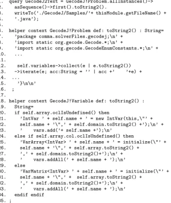
ATL is also used to generate the solver target file. This is possible by defining a new ATL file (called generically ATL2Text) where we can embed the concepts of the metamodel in the syntax of the target file. This is done by means of a querying facility that enables to specify requests onto models.
1. query GecodeJ2Text = GecodeJ!Problem.allInstances()-> 2. asSequence()->first().toString2().
3. writeTo(’./GecodeJ/Samples/’+ thisModule.getFileName() + 4. ’.java’);
5.
6. helper context GecodeJ!Problem def: toString2() : String= 7. ’package comma.solverFiles.gecodej;\n’ +
8. ’import static org.gecode.Gecode.*;\n’ +
9. ’import static org.gecode.GecodeEnumConstants.*;\n’ + 10. ...
11.
12. self.variables->collect(e | e.toString2()) 13. ->iterate(e; acc:String = ’’ | acc +’ ’+e) + 14. ...
15. ’}\n\n’ 16. ; 17.
18. helper context GecodeJ!Variable def: toString2() : 19. String=
20. if self.array.oclIsUndefined() then
21. ’IntVar ’ + self.name + ’ = new IntVar(this,\"’ + 22. self.name + ’\",’ + self.domain.toString2() +’);\n’ + 23. ’ vars.add(’+ self.name +’);\n’
24. else if self.array.col.oclIsUndefined() then
25. ’VarArray<IntVar> ’ + self.name + ’ = initialize(\"’ + 26. self.name + ’\",’ + self.array.toString2() +
27. ’,’ + self.domain.toString2()+’);\n’ + 28. ’ vars.addAll(’ + self.name + ’);\n’ 29. else
30. ’VarMatrix<IntVar> ’ + self.name + ’ = initialize(\"’ + 31. self.name + ’\",’ + self.array.toString2() +
32. ’,’ + self.domain.toString2()+’);\n’ + 33. ’ vars.addAll(’ + self.name + ’);\n’ 34. endif endif
35. ;
Figure 12. GecodeJ2Text file
Figure 12 shows a fragment of the GecodeJ2Text definition to generate the Gecode/J file. Lines 1-4 states the query on the
Problemconcept and defines the target file. Queries are able to call helpers, which allow us to build the string to be written in the target solver file. This query calls the helpertoString2()defined for the conceptProblem. This helper is stated at line 6 and it creates first the string corresponding to the headers (package and import state-ments) of a Gecode/J model. Then, at lines 12-13 the string corre-sponding to the variables declarations is created. This is done by iterating the collection of variables and calling the corresponding
toString2()helper for theVariableinstances. This helper is de-clared at line 18, it defines three possible variable declarations, sin-gle variable (IntVar), a one dimension array (VarArray<IntVar>), and a two dimension array (VarMatrix<IntVar>). The alterna-tives are chosen by means of an if-else statement. The condition
self.array.oclIsUndefined()checks whether the concept array is undefined. If this occurs, the variable corresponds to a single vari-able. The string representing this declaration usesself.namewhich refers to the name of the variable,self.domain.toString2()calls a helper to get the string representing the domain of the variable. The next alternative tests if the attributecolof thearrayis unde-fined, in this case the variable is a one dimension array, otherwise it is a two dimension array. The callself.array.toString2()is used in the two last alternatives, it returns the string corresponding to the size of arrays.
Figure 13 depicts an extract of the Gecode/J file generated for the stable marriage problem. Lines 1-3 states the headers. Line 6 declares the array calledman wife. which is initialized with size
5 and domain [1,5]. At line 8 the array is added to a global array calledvarsfor performing the labeling process. Lines 14-19 illustrate some constraints, which are stated by means of thepost
method.
1. package comma.solverFiles.gecodej; 2. import static org.gecode.Gecode.*;
3. import static org.gecode.GecodeEnumConstants.*; 4. ... 5. 6. VarArray<IntVar> man_wife = 7. initialize("man_wife",5,1,5); 8. vars.addAll(man_wife); 9. 10. VarArray<IntVar> woman_husband = 11. initialize("woman_husband",5,1,5); 12. vars.addAll(woman_husband); 13.
14. post(this, new Expr().p(get(this,woman_husband, 15. get(man_wife,1))),IRT_EQ, new Expr().p(1)); 16. post(this, new Expr().p(get(this,woman_husband, 17. get(man_wife,2))),IRT_EQ, new Expr().p(2)); 18. post(this, new Expr().p(get(this,woman_husband, 19. get(man_wife,3))),IRT_EQ, new Expr().p(3)); 20. ...
Figure 13. Gecode/J model for the stable marriage problem.
4.3 TCS
TCS [19] (Textual Concrete Syntax) is another language provided by the AMMA platform. TCS is not mandatory to add a new translator but it is involved in the process since it is the language used to parse theFlat s-COMMAfile. TCS is able to perform this
task by bridging theFlat s-COMMA metamodel with theFlat s-COMMAgrammar. 1. template Problem 2. : "variables" ":" variables 3. "constraints" ":" constraints 4. "enum-types" ":" enumTypes 5. ; 6. 7. template Variable
8. : type name (isDefined(array) ? array) "in" domain ";" 9. ;
10.
11. template Array
12. : "[" row (isDefined(col) ? "," col ) "]" 13. ;
Figure 14. TCS for Flat s-COMMA.
Figure 14 shows an extract of the TCS file forFlat s-COMMA.
Each class of theFlat s-COMMAmetamodel has a dedicated
tem-plate declared with the same name. Within temtem-plates, words be-tween double quotes are tokens in the grammar (e.g."variables",
":"). Words without double quotes are used to introduce the cor-responding list of concepts. For instancevariablesis defined as a
reference to objects Variable in the classProblem of the meta-model. Thus, variablesis used to call their associate template i.e., the Variable template. This template defines the syntactic structure of a variable declaration. It has a conditional structure ((isDefined(array) ? array)), which means that the template
Arrayis only called if the variable is defined as an array.
4.4 Transformation process
TCS and KM3 work together and their compilation generates a Java package (which includes lexers, parsers and code generators) for
Flat s-COMMA(FsC), which is then used by the ATL files to
gen-erate the target model. Figure 15 depicts the complete transforma-tion process. TheFlat s-COMMAfile is the output of thes-COMMA GUI, this file is taken by the Java package which generates a XMI3 (XML Metadata Interchange) forFlat s-COMMA, this file includes an organized representation of models in terms of their concepts in order to facilitate the task of transformation rules. Over this file ATL rules act and generate a XMI file for Gecode/J. Finally this file is taken by the Gecode/J2Text which builds the solver file.
Figure 15. The AMMA model-driven process on the example of
Flat s-COMMA (FsC) to Gecode/J.
The complete process involves TCS, KM3 and ATL. But, the integration of a new translator just requires KM3 and ATL (the mapping tool only needs one TCS file). As we mention in Sec-tion 4.2, solver metamodels are almost equivalents, and ATL rules are mainly one to one mappings. As a consequence, the develop-ment of KM3 and ATL rules for new solver-translators should not be a hard task. So, we could say that the concrete work for plugging a new solver is reduced to the definition of the ATL2Text file.
Currently, There are two versions of our mapping tool, one with AMMA translators and one with translators written by hand (in Java), which we got from a preliminary development phase of the system. Comparing both approaches, let us make the following concluding remarks.
•The development of hand-written translators is in general a hard task. Their creation, modification and reuse require to have a deep insight in the code and in the architecture of the platform, even more if they have a specific and/or complex design. For instance, the developer may be forced to directly use lexers and parsers, or a given library which provides specific methods to generates the target files.
•The development of AMMA translators does not require ad-vanced language implementation skills. We show that the use of KM3 and ATL is not really a hard task. Moreover, AMMA is supported by a set of tools [7] which provide a great framework to create and manipulate KM3, ATL and TCS models, and also for project handling. An independent definition of syntax con-cerns (ATL2Text) from metamodel concepts (KM3) is another advantage which gives us a more organized view that facilitates the creation and reuse of translators.
3XMI is the standard used for exchanging metadata in MDD architectures.
• The development of hand-written translators requires more code lines. In our implementation, the source files of Java trans-lators are approximately 60% bigger than the AMMA transla-tors source files (ATL+KM3).
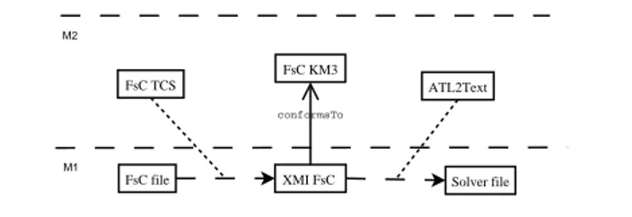
4.5 Direct code generation
There is another approach to develop translators using the AMMA platform. For instance, if we want to use just theFlat s-COMMA
features that are supported by the solver, we can omit the transfor-mation rules and we can apply the ATL2Text directly on the source metamodel. Figure 16 shows this direct code generation process.
FsC KM3
XMI FsC conformsTo
FsC file Solver file
FsC TCS ATL2Text
M1 M2
Figure 16. Direct code generation.
Although this approach is simpler, it is less flexible since we lose the possibility of using interesting rules transformations such as the set matrix decomposition explained in Section 4.2.
5.
Experiments
We have carried out a set of tests in order to first compare the performance of AMMA translators (using transformation rules) with translators written by hand, and second, to show that the automatic generation of solver files does not lead to a loss of performance in terms of solving time. Tests have been performed on a 3GHz Pentium 4 with 1GB RAM running Ubuntu 6.06, and benchmarks used are the following [28]:
• Send: The cryptoarithmetic puzzle Send + More = Money.
• Stable: The stable marriage problem presented.
• Queens: The N-Queens problem (n=10 and n=18).
• Packing: Packing 8 squares into a square of area 25.
• Production: A production-optimization problem.
• Ineq20: 20 Linear Inequalities.
• Engine: The assembly of a car engine subject to design con-straints.
• Sudoku: The Sudoku logic-based number placement puzzle.
• Golfers: To schedule a golf tournament.
Table 1. Translation times (seconds)
sC to FsC to Gecode/J FsC to ECLi
PSe
Benchmark FsC Java AMMA Java AMMA Send 0.237 0.052 0.688 0.048 0.644 Stable 0.514 0.137 1.371 0.143 1.386 10-Queens 0.409 0.106 1.301 0.115 1.202 18-Queens 0.659 1.122 3.194 0.272 2.889 Packing 0.333 0.172 1.224 0.133 1.246 Production 0.288 0.071 0.887 0.066 0.783 20 Ineq. 0.343 0.072 0.895 0.072 0.891 Engine 0.285 0.071 0.815 0.071 0.844 Sudoku 3.503 1.290 4.924 0.386 4.196 Golfers 0.380 0.098 1.166 0.111 1.136
Table 1 shows preliminary results comparing AMMA transla-tors with translatransla-tors written by hand (in Java). Column 3 and 4 give the translation times using Java and AMMA translators, from
Flat s-COMMA(FsC) to Gecode/J and from Flat s-COMMA to ECLi
PSe
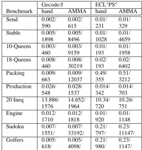
Table 2. Solving times(seconds) and model sizes (number of
to-kens)
Gecode/J ECLi
PSe
Benchmark hand AMMA hand AMMA Send 0.002/ 0.002/ 0.01/ 0.01/ 590 615 231 329 Stable 0.005/ 0.005/ 0.01/ 0.01/ 1898 8496 1028 4659 10-Queens 0.003/ 0.003/ 0.01/ 0.01/ 460 9159 193 1958 18-Queens 0.008/ 0.008/ 0.02/ 0.02/ 460 30219 193 6402 Packing 0.009/ 0.009/ 0.49/ 0.51/ 663 12037 355 3212 Production 0.026/ 0.028/ 0.014/ 0.014/ 548 1537 342 703 20 Ineq 13.886/ 14.652/ 10.34/ 10.26/ 1576 1964 720 751 Engine 0.012/ 0.012/ 0.01/ 0.01/ 1710 1818 920 1148 Sudoku 0.007/ 0.007/ 0.21/ 0.23/ 1551/ 33192/ 797/ 11147/ Golfers 0.005/ 0.005/ 0.21/ 0.23/ 618/ 4098/ 980/ 1147/
Flat s-COMMAare given for reference in column 2 (This process involves syntactic and semantic checking, and the transformations explained in Section 3.3). The results show that AMMA transla-tors are slower than Java translatransla-tors, this is unsurprising since Java translators have been designed specifically for s-COMMA. They take as input aFlat s-COMMAdefinition and generate the solver file directly. The transformation process used by AMMA translators is not direct, it performs intermediate phases (XMI to XMI). More-over, the AMMA tools are under continued development and many optimizations can be done especially on the parsing process of the source file (more than 60% of the time is consumed by this pro-cess). Although our primary scope is not focused on performance, we expect to improve this using the next AMMA version.
However, despite of this speed difference, we believe translation times using AMMA are acceptable and this loss of performance is a reasonable price to pay for using a generic approach.
In Table 2 we compare the solver files generated by AMMA translators4 with native solver files version written by hand. The data is given in terms of solving time(seconds)/model size(tokens). Results show that generated solver files are in general bigger than solver versions written by hand. This is explained by the loop unrolling and flattening composition processes presented in Sec-tion 3.3. However, this increase in terms of code size does not cause a negative impact on the solving time. In general, generated solver versions are very competitive with hand-written versions.
Table 2 also shows that Gecode/J files are bigger than ECLiPSe files, this is because the Java syntax is more verbose than the ECLi
PSe
syntax.
6.
Related Work
s-COMMAis as related to solver-independent languages as
object-oriented languages. In the next paragraphs we compare our ap-proach to languages belonging to these groups.
4In the comparison, we do not consider solver files generated by Java translators. They do not have relevant differences compared to solver files generated by AMMA translators.
6.1 Solver-Independent Constraint Modeling
Solver-independence in constraint modeling languages is a recent trend. Just a few languages have been developed under this prin-ciple. One example is MiniZinc, which is mainly a subset of con-structs provided by Zinc, its syntax is closely related to OPL and its solver-independent platform allows to translate models into Gecode and ECLiPSesolver code. This model transformation is performed by a rule-based system called Cadmium [5] which can be regarded as an extension of Term-Rewriting (TR) [2] and Constraint Han-dling Rules (CHR) [11]. This process also involves an interme-diate model called FlatZinc, which plays a similar role thanFlat s-COMMA, to facilitate the translation.
The implementation of our approach is quite different to Cad-mium. While Cadmium is supported by CHR and TR, our approach is based on standard model transformation techniques, which we believe give us some advantages. For instance, ATL and KM3 are strongly supported by the model engineering community. A consid-erable amount of documentation and several examples are available at the Eclipse IDE site [7]. Tools such as Eclipse plug-ins are also available for developing and debugging applications. It is not less important to mention that ATL is considered as a standard solution for model transformation in Eclipse.
On the technical side, the Cadmium system is strongly tied to MiniZinc. This is a great advantage since the rules operate directly on Zinc expression, so transformation rules are often compact. However, this integration forces to merge the metamodel concepts of MiniZinc with the MiniZinc syntax. This property makes Cad-mium programs more compact but less modular than our approach, where the syntax is defined independently from the metamodel (as we have presented in Section 4).
Essence is another solver-independent language. Its syntax is addressed to users with a background in discrete mathematics, this style makes Essence a specification language rather than a model-ing language. The Essence execution platform allows to map spec-ifications into ECLiPSeand Minion solver [13]. A model transfor-mation system called Conjure has been developed, but the integra-tion of solver translators is not its scope. Conjure takes as input an Essence specification and transform it to an intermediate OPL-like language called Essence’. Translators from Essence’ to solver code are written by hand.
From a language standpoint, s-COMMA is as expressive as MiniZinc and Essence, in fact these approaches provide similar constructs and modeling features. However, a main feature of
s-COMMAthat strongly differences it from aforementioned lan-guages is the object-oriented framework provided and the possibil-ity of modeling problems using a visual language.
6.2 Object-Oriented Constraint Modeling and Visual Environments
The capability of defining constraints in an object-oriented mod-eling language is the base of the object-oriented constraint model-ing paradigm. The first attempt in performmodel-ing this combination was on the development of ThingLab [3]. This approach was designed for interactive graphical simulation. Objects were used to represent graphical elements and constraints defined the composition rules of these objects.
COB [16] is another object-oriented language, but its frame-work is not purely based on this paradigm. In fact, the language is a combination of objects, first order formulas and CLP (Constraint Logic Programming) predicates. A GUI tool is also provided for modeling problems using CUML, a UML-like language. The fo-cus of this language was the engineering design. Modelica [10] is another object-oriented approach for modeling problems from the engineering field, but it is mostly oriented towards simulation.
Gianna [25] is a precursor visual environment for modeling CSP. But its modeling style is not object-oriented and the level of abstraction provided is lower than in UML-like languages. In this tool, CSPs are stated as constraint graphs where nodes represent the variables and the edges represent the constraints.
Although these approaches do not have a system to plug-in new solvers and were developed for a specific application domain, we believe it is important to mention them.
It is important to clarify too, that object-oriented capabilities are also provided by languages such as CoJava [4]; and in libraries such as Gecode or ILOG SOLVER. The main difference here is that the host language provided is a programming language but not a high-level modeling language. As we have explained in Section 1, advanced programming skills may be required to deal with these tools.
7.
Conclusions and Future Work
In this work we have presenteds-COMMA, an extensible MDD
platform for modeling CSPs. The whole system is composed by two main parts: A modeling tool and a mapping tool, which provide to the users the following three important facilities:
•A visual modeling language that combines the declarative as-pects of constraint programming with the useful features of object-oriented languages. The user can state modular models in an intuitive way, where the compositional structure of the problem can be easily maintained through the use of objects under constraints.
•Models are stated independently from solver languages. Users are able to design just one model and to target different solvers. This clearly facilitates experimentation and benchmarking.
•A model transformation system supported by the AMMA plat-form which follows the standards of the software engineering field. The system allows users to plug-in new solvers without writing translators by hand.
Currently, we do not uses-COMMAas our source model, be-cause its metamodel is quite large and defining generic mappings to different solver metamodels will be a serious challenge. However we believe that this task will lead to an interesting future work, for instance to perform reverse engineering (e.g. Gecode/J to s-COMMAor ECLiPSetos-COMMA). The use of AMMA for model
optimization will be useful too, for instance to eliminate redundant or useless constraints. The definition of selective mappings is also an interesting task, for instance to decide, depending on the solver used, whether loops must be unrolled or the composition must be flattened.
Acknowledgments
We are grateful to the support of this research from the “Pontifi-cia Universidad Cat´olica de Valpara´ıso” under the grant “Beca de Estudios B´asica”, and to Fr´ed´eric Jouault for his support on the implementation of the AMMA translators.
References
[1] ANTLR Reference Manual, 2007. http://www.antlr.org.
[2] F. Baader and T. Nipkow. Term rewriting and all that, Cambridge Univ. Press, 1998.
[3] A. Borning. The Programming Languages Aspects of ThingLab, a Constraint-Oriented Simulation Laboratory. ACM Transactions on
Programming Languages and Systems (ACM TOPLAS), 3(4), pages
353–387, 1981.
[4] A. Brodsky and H. Nash. CoJava: Optimization Modeling by Nondeterministic Simulation. In Proceedings of the 12th International
Conference on Principles and Practice of Constraint Programming (CP 2006) 3(4). LNCS, vol. 4204, pages 91–106, 2006.
[5] S. Brand, G. J. Duck, J. Puchinger and P. J. Stuckey. Flexible, Rule-Based Constraint Model Linearisation. In Proceedings of the 10th
Symposium on Practical Aspects of Declarative Languages (PADL 2008). LNCS, vol. 4902, pages 68–83, 2008.
[6] D. Diaz and P. Codognet. The GNU Prolog System and its Imple-mentation. In Proceedings of the 2000 ACM Symposium on Applied
Computing (SAC 2000), pages 728–732, 2000.
[7] Eclipse Model-to-model transformation, 2008. http://www.eclipse.org/m2m/.
[8] A. M. Frisch, C. Jefferson, B. Mart´ınez Hern´andez and I. Miguel. The Rules of Constraint Modelling. In Proceedings of the 19th International
Joint Conference on Artificial Intelligence (IJCAI 2005), pages 109–116,
2005.
[9] A. M. Frisch, M. Grum, C. Jefferson, B. Mart´ınez Hern´andez and I. Miguel. The Design of ESSENCE: A Constraint Language for Specifying Combinatorial Problems. In Proceedings of the 20th
International Joint Conference on Artificial Intelligence (IJCAI 2007),
pages 80–87, 2007.
[10] P. Fritzson and V. Engelson. Modelica – A Unified Object-Oriented Language for System Modeling and Simulation. In Proceedings of the
12th European Conference on Object-Oriented Programming (ECOOP 1998). LNCS, vol. 1445, pages 67–90, 1998.
[11] T. W. Fr¨uhwirth. Theory and Practice of Constraint Handling Rules.
Journal of Logic Programming 37(1-3), pages 95–138, 1998.
[12] Gecode System, 2006. http://www.gecode.org.
[13] I. P. Gent, C. Jefferson and I. Miguel. Minion: A Fast Scalable Constraint Solver. In Proceedings of the 17th European Conference on
Artificial Intelligence (ECAI 2006), pages 98–102, 2006.
[14] L. Granvilliers and F. Benhamou. Algorithm 852: RealPaver: an interval solver using constraint satisfaction techniques. ACM Transactions on Mathematical Software (ACM TOMS), 32(1), pages
138–156, 2006.
[15] J. Jaffar and J.-L. Lassez. Constraint Logic Programming. In
Proceedings of the 14th Annual ACM Symposium on Principles of Programming Languages (POPL 1987), pages 111–119, 1987.
[16] B. Jayaraman and P. Tambay. Modeling Engineering Structures with Constrained Objects. In Proceedings of the 4th Symposium on Practical
Aspects of Declarative Languages (PADL 2002). LNCS, vol. 2257,
pages 28–46, 2002.
[17] F. Jouault and I. Kurtev. Transforming Models with ATL. In
Proceedings of Satellite Events at the 8th International Conference on Model Driven Engineering Languages and Systems (MoDELS Satellite Events 2005). LNCS, vol. 3844, pages 128–138, 2005.
[18] F. Jouault and J. B´ezivin. KM3: A DSL for Metamodel Specification. In Proceedings of the 8th IFIP WG 6.1 International Conferenceon
Formal Methods for Open Object-Based Distributed Systems (FMOODS 2006). LNCS, vol. 4037, pages 171–185, 2006.
[19] F. Jouault, J. B´ezivin and I. Kurtev KM3: A DSL for Metamodel Specification. In Proceedings of the 5th International Conference on
Generative Programming and Component Engineering (GPCE 2006),
pages 249–254, 2006.
[20] I. Kurtev, J. B´ezivin, F. Jouault and P. Valduriez. Model-based DSL frameworks. In Proceedings of Companion to the 21th Annual
ACM SIGPLAN Conference on Object-Oriented Programming, Systems, Languages, and Applications (OOPSLA Companion 2006), pages 602–
616, 2006.
[21] N. Nethercote, P. J. Stuckey, R. Becket, S. Brand, G. J. Duck and G. Tack. MiniZinc: Towards a Standard CP Modelling Language. In
Proceedings of the 13th International Conference on Principles and Practice of Constraint Programming (CP 2007) 3(4). LNCS, vol. 4741,
pages 529–543, 2007.
http://www.omg.org/cgi-bin/doc?formal/2006-05-01
[23] OMG - The Unified Modeling Language (UML) 2.1.1 Infrastructure Specification, 2007. http://www.omg.org/spec/UML/2.1.2/.
[24] OMG - Model Driven Architecture (MDA) Guide V1.0.1, 2003 http://www.omg.org/cgi-bin/doc?omg/03-06-01.
[25] M. Paltrinieri. A Visual Constraint-Programming Environment. In
Proceedings of the 1st International Conference on Principles and Practice of Constraint Programming (CP 1995) 3(4). LNCS, vol. 976,
pages 499–514, 1995.
[26] J.-F. Puget. A C++ implementation of CLP. In Proceedings of the
Second Singapore International Conference on Intelligent Systems (SCIS 1994), 1994.
[27] R. Rafeh, M. J. Garc´ıa de la Banda, K. Marriott and M. Wallace. From Zinc to Design Model. In Proceedings of the 9th Symposium on
Practical Aspects of Declarative Languages (PADL 2007). LNCS, vol.
4354, pages 215–229, 2007.
[28] s-COMMA System, 2008. http://www.inf.ucv.cl/˜rsoto/s-comma. [29] R. Soto and L. Granvilliers. The Design of COMMA: An Extensible
Framework for Mapping Constrained Objects to Native Solver Models. In Proceedings of the 19th IEEE International Conference on Tools with
Artificial Intelligence (ICTAI 2007), pages 243–250, 2007.
[30] P. Van Hentenryck. The OPL Language. MIT Press, 1999. [31] M. Wallace, S. Novello and J. Schimpf. Technical report, IC-Parc,