Are any public-reported earthquake precursors valid?

HAL Id: hal-00299148

https://hal.archives-ouvertes.fr/hal-00299148

Submitted on 27 Jul 2004

HAL is a multi-disciplinary open access

archive for the deposit and dissemination of

sci-entific research documents, whether they are

pub-lished or not. The documents may come from

teaching and research institutions in France or

abroad, or from public or private research centers.

L’archive ouverte pluridisciplinaire HAL, est

destinée au dépôt et à la diffusion de documents

scientifiques de niveau recherche, publiés ou non,

émanant des établissements d’enseignement et de

recherche français ou étrangers, des laboratoires

publics ou privés.

Are any public-reported earthquake precursors valid?

N. E. Whitehead, U. Ulusoy, H. Asahara, M. Ikeya

To cite this version:

N. E. Whitehead, U. Ulusoy, H. Asahara, M. Ikeya. Are any public-reported earthquake precursors

valid?. Natural Hazards and Earth System Science, Copernicus Publications on behalf of the European

Geosciences Union, 2004, 4 (3), pp.463-468. �hal-00299148�

© European Geosciences Union 2004

and Earth

System Sciences

Are any public-reported earthquake precursors valid?

1_{Quantum Geophysics Laboratory, Osaka University, Toyonaka, Osaka 5600043, Japan} 2_{Department of Physics Engineering, Hacettepe University, 06532 Beytepe, Ankara, Turkey}

Received: 6 April 2004 – Revised: 21 June 2004 – Accepted: 22 June 2004 – Published: 27 July 2004

Abstract. This article examines retrospective public-supplied precursor reports statistically, and confirms pub-lished hypotheses that some alleged precursors within 100 km and within a day prior to the large 1995 Kobe and 1999 Izmit earthquakes, may be valid. The confirmations are mostly at the p<0.001 level of significance. Most significant were alleged meteorological and geophysical precursors, and less often, animal reports. The chi-squared test used, for the first time eliminates the distorting effects of psychological factors on the reports. However it also shows that correct reports are diluted with about the same number which are merely wishful thinking, and obtaining more reliable data would be logistically difficult. Some support is found for another published hypothesis in which other precursors oc-curred within the ten days prior to the earthquake.

1 Introduction

Most discussions of alleged earthquake precursors have been anecdotal, but some of the larger and more recent sur-veys present summary statistical information and objective testable hypotheses. Tributsch (1984) summarising alleged precursor times from more than 70 historical earthquakes found a mean of 21 h. Rikitake (2001) besides confirm-ing that prior-day pattern, presented data on the distances of precursor reports for several large Japanese earthquakes prior to 1995. For the Ansei-Tokai, Nobi and Great Kanto Earthquakes 82% of reports were of events within 100 km as shown in Fig. 1.

These numerical hypotheses can be tested against other data sets from earthquakes, but they do not deal with the possibility that most reports originate because of mere psy-chological reasons. This paper proposes a way of allowing for the psychological contribution and applies it to the Kobe (M7.3, 17/1/1995) and Izmit (M7.4, 17/8/1999) earthquakes.

Correspondence to: N. E. Whitehead

(whiteh@paradise.net.nz)

2 Methods

Following the Kobe earthquake, a media appeal for eye-witness accounts of alleged precursors yielded 1189 usable statements for time/distance hypothesis testing, which com-pilers divided for convenience into classes: meteorological, geophysical, human, animal, birds, fish, reptiles, insects, plants and sundry, the latter including reports of abnormal radio and TV interference (Wadatsumi, 1995). Wadatsumi’s publication included data from the compilation work of the Kansai Science Forum. The “geophysical” class included subterranean sounds, well water changes and sea anomalies. The exact number of reports usable depended on whether times and distances were submitted in sufficient detail.

Other workers independently collected reports for the Izmit earthquake and compiled another 664 eyewitness ac-counts, similarly divided into several classes (Ulusoy and Ikeya, 2001). For neither earthquake were reports edited and rejected even though many were arguably describing com-mon events, assumed by respondents to be significant and precursory. Testing using unedited raw data is one com-monly accepted procedure within the discipline of survey techniques. Imposed selection criteria might have sharpened still further the results which follow but they would be sub-ject to debate.

Chi-squared tests were used, which do not depend on any particular shape or symmetry being present in the data. The first test compared the relative numbers in the various classes for reports within and beyond 100 km, (regardless of when they occurred) and the second compared the relative numbers in classes for reports from the day before, with all other times (regardless of the distance of occurrence).

The 100 km test limit was also supported by three con-siderations independent of Tributsch (1984) and Rikitake (2001). Firstly in our experience for an earthquake of M7.4, (e.g. Izmit), a 100 km radius includes almost all visual effects in the geosphere such as landslides and earth fissures, and ar-guably any mechanisms contributing to precursors. Secondly about 70% of the reports from the Kobe earthquake and Izmit

464 N. E. Whitehead et al.: Are any public-reported earthquake precursors valid?

Table 1. Chi-squared distance analysis for Izmit earthquake reports (all precursor times combined).

Observed <101 km Expected for >100 km Observed >100 km Chisquared

Meteorological 120 54.35 62 1.075 Geophysical 65 29.44 17 0.856 Animals 242 109.61 112 0.051 Electronic 30 13.58 16 0.427 Totals: 457 207 207 2.411 p = 0.146

Table 2. Chi-squared analysis of Izmit earthquake data for test distance of 90 km.

Observed <91 km Expected for >90 km Observed >90 km Chisquared

Animals 145 174.4 209 4.94 Meteorological 82 83.4 100 0.024 Geophysical 59 19.2 23 82.60 Electronic 16 25.02 30 3.26 Totals: 302 302 362 90.83 p= 1.45×10−19

Fig. 1. Distribution of precursor reports. Distances from epicentre

(from data in Rikitake, 2001).

earthquake were from 100 km or less and it was undesirable to decrease the statistical power of the chi-squared test by making the test distance larger and further unbalancing the ratio of reports from inside and outside 100 km. Thirdly data from an independent survey on disturbed sleep patterns in the Kobe-Osaka region before the earthquake (Ikeya, in prepara-tion, 20031) suggested a cut-off for any effect at 100 km.

There were two similar null hypotheses for the test. The first was that the proportion of the number of reports in dif-ferent classes was merely due to psychological invention, and would not differ regardless of distance of reported precur-sor before the earthquake. The second was similarly that the proportion of the number of reports in different classes was 1_{Ikeya, M.: Sleep patterns before Kobe earthquake, in}

Earth-quake Precursors, Kerala, India, 2005.

merely due to psychological invention, and would not differ regardless of the time of reported precursors before the earth-quake. Significant deviations would indicate the presence of possible precursors (though possibly diluted by mistaken re-ports).

There are no surveys which have specifically checked the null hypotheses. However if meteorological etc. conditions for a range of days before an earthquake are similar, it seems reasonable that the proportions of reports in different classes should be similar. Similarly if the conditions are similar over a range of distances, it seems reasonable that proportions of reports in different classes should be similar.

Following the main statistical tests, it was possible to ex-plore the data and it will be shown that this provided further evidence that the null hypotheses were reasonable.

The basic assumption of uniformity with distance was vi-olated for the Kobe region for one class of reports about fish, because most reports from more than 50 km away were in-land, and could not furnish fish observations. The effects of this factor were checked.

There was a large anticyclone over the survey areas in both countries during the earthquake period giving relatively sta-ble and uniform weather for hundreds of kilometres, support-ing the idea of constant conditions inside and outside the test distance.

Report classes for the chi-squared test were combined if necessary to achieve minimum frequencies per cell of 4. Calculations used Excel spreadsheets including the function CHITEST for calculating chi-squared significance probabil-ities. Reports were rare events from large media audiences, hence they are a classic case of Poisson statistics, i.e. the errors on numbers of reports in Tables 1–5 which follow, are the square root of the numbers, hence relatively small,

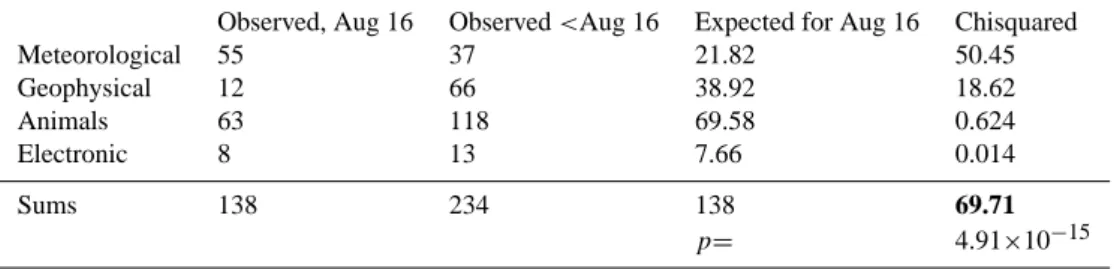
Table 3. Izmit earthquake chi-squared time test.

Observed, Aug 16 Observed <Aug 16 Expected for Aug 16 Chisquared

Meteorological 55 37 21.82 50.45 Geophysical 12 66 38.92 18.62 Animals 63 118 69.58 0.624 Electronic 8 13 7.66 0.014 Sums 138 234 138 69.71 p= 4.91×10−15

meaning relative proportions in the absence of precursors should be moderately stable. Chi-squared tests presented later similarly indicate that proportions in the classes would not fluctuate wildly under identical resampling. The special strength of the chi-squared technique is that since it looks at relative proportions in different classes it does not matter if absolute report numbers differ with distance.

3 Results and discussion

3.1 Izmit earthquake

3.1.1 Izmit earthquake: distance analysis

The first chi-squared tests used the Izmit earthquake data with the results shown in Table 1. Expected values for re-ports at >100 km were calculated by proportion from data at <100 km. Similar calculations for expected values were per-formed for Tables 2–6. Where the figure “<101 km” occurs it means distances of 100 km and below. Where “>100 km” occurs it means distances of 101 km and above.

Please note that classifications cannot be the same for all tables, because it was necessary to combine some classifica-tions to achieve the minimum report numbers necessary for a valid chi-squared test

The Chi-squared result of 0.146 for the four classes was not significant at the p=0.05 level. We therefore cannot reject the null hypothesis that the two distance classes are the same, i.e. no effect of the earthquake has been reported.

Subsequent investigation of how chi-squared changed with distance showed that the choice of 100 km as a test distance was not quite optimum for this set of data. It would have been dramatically more significant to choose 90 km instead, which is a rather small change from 100 km. For a test distance of 90 km the chi-squared value increased to a very high 91 (p=1×10−19). Choosing a variety of test distances showed that at 90 km and below, highly significant chi-squared val-ues were obtained and at 100 km and above, non-significant values of chi-squared were obtained. The results are shown in graphical form in Fig. 2.

For 100 km and above, low chi-squared values result and this shows the null hypothesis is reasonable. Above 100 km proportions in report classes do not differ from each other with change in distance. Distances below 90 km are dramat-ically different. However to follow good statistical practice,

Fig. 2. Change of chi-squared with distance (Izmit earthquake data).

The ordinate here and in later Figs. 3–4 is the reciprocal of the sig-nificance level for each chi-squared value.

in which test hypotheses should be selected beforehand and not altered part way through, we are forced to use the 100 km test distance on the Kobe earthquake data also.

The detailed figures and chisquared test for the revised dis-tance of 90 km are in Table 2.

The high chi-squared result in Table 2 was overwhelm-ingly caused by a relatively much greater number of reports of unusual sea phenomena (“geophysical”) from within 90 km, specifically “death waves”, mini-tsunamis well known in the area as alleged precursors of large earthquakes, which in this case caused well documented damage above usual tide limits.

3.1.2 Izmit earthquake: time analysis

A test for precursor reports on the last day before the Izmit earthquake (Table 3), combining appropriate data, gave a chi-squared of 69.7 (p=14.9×10−15)which is highly significant and supported the hypothesis that reports from the day be-fore the earthquake contain precursors. Meteorological and geophysical reports gave the largest contribution to the chi-squared result.

3.1.3 Earlier precursors

A subsidiary testable hypothesis in Rikitake (2001) was that other precursors might exist in significant numbers, back to a

466 N. E. Whitehead et al.: Are any public-reported earthquake precursors valid?

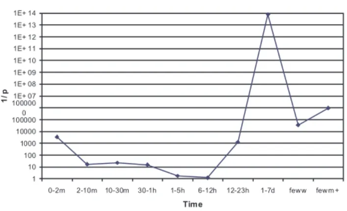
Fig. 3. Change of chi-squared with precursor time (Izmit

earth-quake).

limit of ten days before the earthquake. To test this, the data for the previous day were divided into smaller time classes and each was compared with all other times. The results are in Fig. 3 and show that the point of most significance is outstandingly 1–7 day so Rikitake’s hypothesis was con-firmed for the Izmit earthquake. The reason is again the death waves, but meteorological phenomena were also even more important (see Table 3), and these consisted mainly of vari-ous unusual colours and lights seen in the sky.

3.2 Kobe earthquake

3.2.1 Kobe earthquake: distance analysis

Following the Izmit earthquake calculations, the hypotheses were tested against the Kobe earthquake data which existed in slightly more detailed classes than the Izmit earthquake data. The data used for testing the distance hypothesis are in Table 4.

This very high chi-squared of 117, is consistent with real precursors for a distance of 100 km. It is mainly accounted for by a very large number of meteorological reports, but Ta-ble 4 shows they are from outside 100 km rather than inside 100 km. This seemed at first to disprove a hypothesis which says the phenomena are inside 100 km, but when the original reports were re-read, this is not so. The reports from outside 100 km were of unusual cloud patterns (mainly out-of-season towering cumulus) occurring within 100 km, which could not be seen inside 100 km because the observers were right un-derneath. Probably these reports should have been reclassi-fied as reports from inside 100 km. This means there were indeed statistically significant occurrences within 100 km.

Two other distance tests were possible given the classifica-tion of the data, and the three were all highly significant be-cause of excess meteorological reports: <50 km Chi-squared 103 (p=2×10−19), <100 km chi-squared 117 (p=1x10−23) and <200 km, chi-squared 90 (p=1×10−16). This test shows within its limited range, that 100 km was optimum, but more detailed classes were not possible due to lack of information in the database. There appeared to be significant

contribu-Fig. 4. Change of chi-squared with precursor time (Kobe

earth-quake). There are no data for 11 January.

tions to chi-squared from excess animal, bird and similar re-ports at <100 km.

3.2.2 Kobe earthquake: time analysis

The Kobe earthquake data were available mostly in daily time divisions and were not always strictly identical with the Izmit earthquake data. The data from the day before the earthquake were compared with all other prior data as shown in Table 5 below.

The chi-squared value of 29.7 (p=5×10−4)is high, con-firming the hypothesis that the day before the earthquake contains significant precursors. Alleged electronic precur-sors within the “sundry” class predominate.

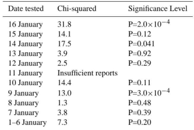
3.2.3 Kobe earthquake: earlier possible precursors The results of testing the 10-day hypothesis of Rikitake (2001) are below in Table 6, and Fig. 4, including an extra point i.e. 1–6 January 1995, to complete coverage of January. The figure shows a peak on 9 January 1995 with chi-squared of 13.0 (p=3.0×10−4_{). Re-reading the original} re-ports shows this peak is due to an excess of meteorological reports on the 9 January which are absent on the 16 Jan-uary. Agreeing with Rikitake’s hypothesis, there is indeed a second alleged precursor peak within the previous 10 days (the small peak on 14 January is only marginally significant). The above results were confirmed by data from December (not shown) in which no significant chi-squared results were found. So 9 January and 16 January were anomalous but no other day right back to the beginning of December.

Only two days out of the six weeks before the Kobe Earth-quake are anomalous. For all the other days the proportions of reports in the various classes remain similar. This sup-ports the null hypothesis that the proportions will not usually change with time before an earthquake.

The high number of precursors on 9 January 1995 coin-cides with abnormal electrical activity in the atmosphere (TV interference etc.) as reported by others (Wadatsumi, 1995; Nagao et al., 2002).

Table 4. Chi-squared analysis for possible distance effects connected with the Kobe earthquake.

Observed <101 km Observed >100 km Expected for >100 km Chi-squared

Meteorological 249 85 31.9 88 Geophysical 89 9 11.4 0.5 Human 69 6 8.8 0.9 Animal 261 16 33.4 9.0 Bird 213 12 27.2 8.5 Sundry* 173 7 22.2 10.0 Totals: 1054 135 135 117 p= 8.88×10−24

Table 5. Chi-squared analysis for 16 January 1995. Alleged precursors for the Kobe Earthquake.

Observed, Jan 16t h Observed Earlier data Expected Earlier data Chi-squared

Meteorological 138 116 124.1 0.54 Geophysical 38 33 34.2 0.042 Human 35 15 31.5 8.64 Animal 104 86 93.6 0.61 Birds 102 103 91.8 1.37 Fish 34 28 30.6 0.22 Reptiles 5 7 4.5 1.39 Fish+Plants 14 21 12.6 5.6 Sundry 19 31 17.1 11.3 Sum: 489 440 440 29.7 p= 0.000489

* This comprised reports involving fish, reptiles, insects, plants and electronic anomalies.

3.3 Psychological contribution

The proportion of reports between classes mostly does not differ for various large distances or times away from the earthquake occurrence and we assume that this distribution is due to psychological invention, that is, a preference for thinking some particular types of event are more likely to be precursors than others. This seems to depend on different na-tional psychological characteristics. For the Kobe earthquake (e.g. Table 5) the order of report popularity was Meteorolog-ical > Birds > Animals, however for the Izmit earthquake (Table 3) it was Animals (including birds) > Geophysical > Meteorological. Detailed reasons for this ordering would be interesting to discuss but are beyond the scope of this paper. Generally the reports consist of the ones due to psycholog-ical invention and the ones on actual precursors. The number of reports for the precursors is found by subtracting the ex-pected psychological numbers from the total number of re-ports. Thus in Table 5, under “Sundry”, there should be 13 precursors because in the total of 31 “observed”, the “ex-pected” 17 reports are taken to be of psychological origin. An examination of all the tables shows that the largest ratio between observed and expected results is 2–3. This means that even for the most significant results 30–50% are of psy-chological origin and 50–70% are precursors.

Table 6. Chi-squared analysis of alleged precursor dates for the

Kobe earthquake.

Date tested Chi-squared Significance Level

16 January 31.8 P=2.0×10−4

15 January 14.1 P=0.12

14 January 17.5 P=0.041

13 January 3.9 P=0.92

12 January 2.5 P=0.29

11 January Insufficient reports

10 January 14.4 P=0.11 9 January 13.0 P=3.0×10−4 8 January 1.3 P=0.48 7 January 3.8 P=0.39 1–6 January 7.3 P=0.20 4 Conclusion

This work has found statistical evidence for an excess of pre-cursors reported the day before the Izmit and Kobe earth-quakes, and for a radius of 90 km, implying that real pre-cursors exist. There is good support from both Izmit and Kobe earthquakes for the subsidiary hypothesis that addi-tional significant precursors may exist in the preceding 10 days. The numerical hypotheses in Tributsch (1984) and Rik-itake (2001) are thus mostly confirmed.

468 N. E. Whitehead et al.: Are any public-reported earthquake precursors valid?

The number of mistaken correlations or valid precursor re-ports can be approximately quantified by the above method, but show that valid reports are diluted with almost an equal number of spurious reports, so false alarms using this basis would be common. However it is intriguing and unusual that a sociological method (solicited reports from the public) can provide some backing for alleged physical events. Such a method cannot indicate any mechanism for precursor phe-nomena, for which other discussions must be consulted (e.g. Ikeya, 2004).

A dense network of observers would be necessary to achieve more precise results or use the results in any practical way; probably about a few hundred in every likely epicenter area, and this is probably not logistically feasible.

This article is a further confirmation of an increasing num-ber of objective reports (e.g. Kraemer et al., 1976 and Yokoi et al., 2003) which contain statistical arguments for the real existence of precursors, although the exact mechanisms are still under debate. The hypotheses should be tested against further data sets. This should be done soon, because it seems likely that if predictions of seismic activity are published in the media as they may increasingly be, they could easily af-fect public attitudes to precursors in unpredictable ways and distort precursor reports (e.g. Varatosos et al., 1996a, 1996b).

Acknowledgements. We wish to thank the media representatives in

Osaka/Kobe and Istanbul/Izmit for their very ready cooperation. N. E. Whitehead wishes to thank the Japanese Society for the Promotion of Science, for a Senior Fellowship in 2003–2004 and U. Ulusoy wishes to thank the Osaka University Frontier Research Projects Center for travel funding.

Edited by: M. Contadakis

Reviewed by: S. Uyeda and P. Varotsos

References

Ikeya, M.: Earthquakes and Animals, World Scientific, Singapore, 285pp, 2004.

Kraemer, H. C., Smith, B. E., and Levine, S.: An animal behaviour model for short term earthquake prediction, in: Abnormal An-imal Behavior prior to Earthquakes, edited by Evernden, J. F., U.S. Department of Commerce, Springfield, Virginia, 231–232, 1976.

Nagao, T., Enomoto, Y., Fujinawa, Y., Hata, M., Hayakawa, M., Huang, Q., Izutsu, J., Kushida,Y., Maeda, K., Oike, K., Uyeda, S., and Yoshino, T.: Electromagnetic anomalies associated with the 1995 Kobe earthquake, J. Geodynamics, 33, 401–411, 2002. Rikitake, T.: Prediction and Precursors of Major Earthquakes, Terra

Scientific, Tokyo, 197pp, 2001.

Tributsch, H.: When the Snakes Awake (Paperback edition), MIT Press, Cambridge, Massachussetts, 248pp, 1984.

Ulusoy, U. and Ikeya, M.: Precursor Statements of Earthquakes, Neyir Publisher, Ankara, Turkey, 297pp, in turkish, 2001. Varotsos, P., Eftaxias, K., and Lazaridou, M.: Reply to “A false

alarm based on electrical activity recorded at a VAN station in northern Greece in December 1990” by Datakpoulos, J. and Stavrakis, G., Geophys. Res. Lett., 23, 1359–1362, 1996a. Varotsos, P., Lazaridou, M., Eftaxias, K., Antonopoulos, G.,

Makris, J., and Kopanas, J.: Short-term earthquake prediction in Greece by seismic electric signals, in: A Critical Review of VAN, (edited by Lighthill, J., World Scientific, Singapore, 29– 76, 1996b.

Wadatsumi, K.: 1519 Statements on Precursors, Tokyo Pub., Tokyo, 266pp, in japanese, 1995.

Yokoi, S., Ikeya, M., Yagi, S., and Nagai, K.: Mouse circadian rhythm before the Kobe earthquake in 1995, J. Bioelectromag-netics, 24, 289–291, 2003.